Article

A Traffic-Load-Based Algorithm for Wireless Sensor Networks’ Lifetime Extension

by
Georgios Tsoumanis
,
Nikolaos Giannakeas
,
Alexandros T. Tzallas
,
Evripidis Glavas
,
Kyriakos Koritsoglou
,
Evaggelos Karvounis
,
Konstantinos Bezas
and
Constantinos T. Angelis
*
Department of Informatics and Telecommunications, School of Informatics and Telecommunications, University of Ioannina, Campus of Arta, GR-47100 Arta, Greece
*
Author to whom correspondence should be addressed.
Information 2022, 13(4), 202; https://doi.org/10.3390/info13040202
Submission received: 28 February 2022 / Revised: 4 April 2022 / Accepted: 12 April 2022 / Published: 15 April 2022

Abstract

:
It has been shown in the literature that the lifetime of a wireless sensor network is heavily connected to the number of transmissions that network nodes have to undertake. Considering this finding, along with the effects of the energy hole problem where nodes closer to the sink node transmit more than the more distant ones, a node close to the sink node will be the one that transmits the most, while it will also be the node that will deplete its battery first. Taking into consideration that the failure of a single network node to operate, due to its battery being discharged, can lead to a network stopping its operation, the most energy-consuming node in the network will also be the one that will be responsible for the network’s termination. In this sense, the most energy-consuming node’s energy consumption optimization is the main case in this paper. More specifically, in this work, it is firstly shown that the energy consumption of a wireless sensor network is closely related to each network node’s traffic load, that is the transmissions of the packets that are created or forwarded by a node. The minimization of the most energy-consuming node’s energy consumption was studied here, while the implementation of a traffic-load-based algorithm is also proposed. Under the proposed algorithm, given a simple shortest path approach that assigns a parent (i.e., the next hop towards the sink node) in each network node and the knowledge it provides regarding the distance (in hops in this paper’s case) of network nodes from the sink node, the proposed algorithm exploits the shortest path’s results in order to discover, for all network nodes, neighbors that are of the same distance (from the sink node) with the initially assigned parent. Then, if such neighbors exist, all these neighbors are equally burdened with the parenting role. As a result, the traffic load is shared by all of them. To evaluate the proposed algorithm, simulation results are provided, showing that the goals set were achieved; thus, the network lifetime was prolonged. In addition, it is shown that under the algorithm, a fairer distribution of the traffic load takes place.

1. Introduction

Over the past few years, technological progress in wireless sensor networks has motivated their further growth, their success reflecting the increasing areas of application [1,2]. Apart from technologically growing in terms of applications, wireless devices have also gained attention due to their low cost and small size, allowing for their development in large-scale environments. In wireless networks, energy consumption and energy reservation are of significant importance, but they are even more intense in wireless sensor networks [3] due to these networks’ mainly operating in the absence of any energy supply infrastructure. The latter results in the operation of the wireless devices being entirely dependent on their limited batteries’ energy supply.
While various approaches in the Bibliography study the energy consumption optimization and lifetime prolongation of wireless sensor networks, this paper is deposited next to the traffic-load -balancing-based ones. Usually, in this kind of work, the studied techniques set their goals at balancing the traffic load by either changing the initially assigned traffic load of the network nodes or reverting it, both approaches resulting in a more balanced (among nodes) energy consumption produced by data packet transmissions and receptions. The above goal is approached mainly by pre-defining (or re-defining) the traffic load or re-placing the nodes in the field to balance the traffic load. While these approaches have given some exceptional results, having the ability to place the nodes in pre-defined locations in the field of the network operation or reverting the number of packets nodes created (i.e., the traffic load of nodes) are not always realistic and applicable techniques. For example, changing the initial placement of nodes would be difficult given a network consisting of hundreds of nodes randomly placed in the field. In addition, changing the number of packets that each node creates would also be ineffective in many cases. For example, if the network is operating in a forest and its primary purpose is to trigger an alarm as soon as the temperature value is higher than a given threshold, the packet encapsulating this piece of information would be required to be transmitted as soon as possible along with all the following packets.
Taking the above into consideration, the goal in this paper was threefold. The first goal was to show the connection between traffic load and energy consumption. The second goal was to identify the effects of the most energy-consuming node on the network termination. The third goal was to minimize the energy consumption of the most energy-consuming node by reducing its transmissions and balancing the overall network traffic at the same time. In this sense, a simple-to-implement algorithm is proposed here. While standing next to other traffic-load balancing algorithms, the proposed one’s differentiation mainly lies in its capability to operate on network nodes that have been already placed in the field (i.e., before the operation of the algorithm) and after the initial network traffic load has been set to them. In this sense, a random node placement was considered to be followed by the shortest path approach in order to identify the paths from any node towards the sink node. After collecting the results of the shortest path approach, the proposed algorithm is applied, searching for the possibility of nodes to forward their traffic load towards the sink node through more than one neighbor node, the node’s parents.
The procedure that is followed under the proposed algorithm is straightforward and is given next: At the beginning, the shortest path approach informs nodes about which is their best parent selection. Then, each node, knowing its parent’s distance from the sink node (in hops), searches for other neighbors whose distance in hops from the sink node is the same as the initially assigned parent. If such neighbors exist, all of them are used as parents; thus, the node transmits its data packets to them interchangeably. By applying the above technique, the new parents’ traffic load will be more balanced as they will share the traffic load initially assigned to one of them. Moreover, considering that the data packets will not always be transmitted to the same neighbor, the value of the highest traffic load held by a neighbor will decrease. The network node that holds the highest traffic load is the one that will deplete its battery first, so it will be the one responsible for the network’s termination as well. As a result, minimizing the energy consumption of the most energy-consuming node in each “neighbor” is targeted at eventually resulting in the minimization of the energy consumption of the most energy-consuming node in the network. Another result of the implementation of the proposed algorithm is the overall fairer distribution of the traffic load among nodes, which is achieved by distributing the traffic load that was initially held by a single node to more than one node. Note that the goal here was for the initially assigned traffic load to remain the same for all nodes; what was changed is the cumulative traffic load that is actually the node’s traffic load added to the traffic load of the nodes that uses it as a parent. The cumulative traffic load is thoroughly explained later.
In the sequel, the structure of this paper is given: Recently published relevant works are addressed in Section 2; the considered network is defined in Section 3; the suggested algorithm is detailed in Section 4; the proposed algorithm is evaluated through simulation results in Section 5. The conclusions are drawn in Section 6, and the notations are supplied in Appendix A.

2. Related Work

There has been an interesting literature studying the wireless sensor networks’ lifetime prolongation by balancing nodes’ traffic load [4]. One technique that has been vastly approached is hierarchical clustering [5]. Schemes in hierarchical clustering are generally categorized as cluster-based and grid-based approaches [6]. In the former, nodes are grouped into clusters, where a resourceful sensor node is nominated as a cluster head. In the latter, the network is assumed to be divided into confined virtual grids, a task that in most cases is performed by the base station. A load balancing clustering technique in wireless sensor networks was proposed in [7] by Randhawa and Jain. In this work, the clustering for the load balancing problem was formulated as a multi-objective optimization problem to find an energy-efficient clustering solution. Then, a technique was proposed under which the role of cluster head is shuffled in each round, and new paths are considered based on a weight value assigned for load balancing. In [8], Edla et al. proposed a clustering algorithm that evaluates the particle swarm optimization along with a fitness function that considers the mean cluster distance, gateway load, and the number of heavily loaded gateways in the network.
As for the swarm optimization techniques, Sampathkumar et al. in [9] studied the effective load balancing and routing techniques under the Glowworm swarm optimization approach [10]. Their technique, using a pseudo-random route discovery algorithm and an enhanced pheromone trail-based updating strategy, is targeted at optimizing the sensor nodes’ energy consumption. The proposed technique utilizes a heuristic updating algorithm that bases its operation on cost-effective energy measures to optimize route establishment. Tabibi and Ali, on the other hand, gave a particle-swarm-optimization-based selection approach in their work in [11] to select the optimal “rendezvous” points. Their method is capable of finding optimal or near-optimal “rendezvous” points for efficient network resource management. In addition, for each sensor node, a weight value is calculated considering the data packets it receives from other sensor nodes.
Kacimi et al. in [12] mathematically derived an optimal solution based on load balancing techniques. Then, a distributed heuristic was proposed for approximating the optimal case. By combining load balancing with transmission power control, this heuristic assigns traffic proportions to nodes for better balancing their energy consumption.
An ant-colony-based [13] routing algorithm was proposed in [14] by Li et al. for load balancing the wireless sensor network nodes and achieving a more energy-efficient setup. The proposed algorithm is based on a greedy energy cost metric for optimizing the nodes’ routes’ establishment. In addition, for reducing the energy consumption that is caused by the control overhead, the proposed algorithm utilizes an energy-based opportunistic broadcast scheme.
In order to obtain a better and “fairer” traffic load distribution across nodes, load balancing procedures such as those presented in [15,16,17] have been recommended. In most cases, these approaches are achieved by pre-assigning the desired traffic load on nodes. Clustering approaches (e.g., [18,19]) have been presented in the past for splitting the network into smaller sub-networks to balance the traffic load and reduce energy usage. Furthermore, routing solutions have been developed to prevent the consequences of the energy hole problem (e.g., [20,21]). At the same time, node deployment that focuses on energy consumption optimization (e.g., [22]) has been attempted.
By tackling wireless sensor networks on which traffic loads have already been assigned due to the shortest path technique, the suggested algorithm in this study differs from most current efforts. Furthermore, when the technique is applied, nodes are expected to be uniformly positioned in the field. To the best of the authors’ knowledge, there are no current publications in the literature proposing traffic-load-based algorithms for networks assuming already allocated traffic loads and nodes’ locations. In [23], the notion and theoretical study of using cumulative traffic load as a basis for calculating network node energy consumption was proposed, and in [24], it was further examined. In addition, the extra goal set here was to show that, given predefined nodes’ locations and the packet creation ration (traffic load), under the proposed algorithm, the total packet transmissions, to be later defined as the “cumulative traffic load”, is more fairly allocated among nodes. In this sense, among the various evaluations carried out in this study, the suggested technique’s fairness in terms of the resultant allotted traffic load was also assessed, using the Jain index [25].

3. System Definition
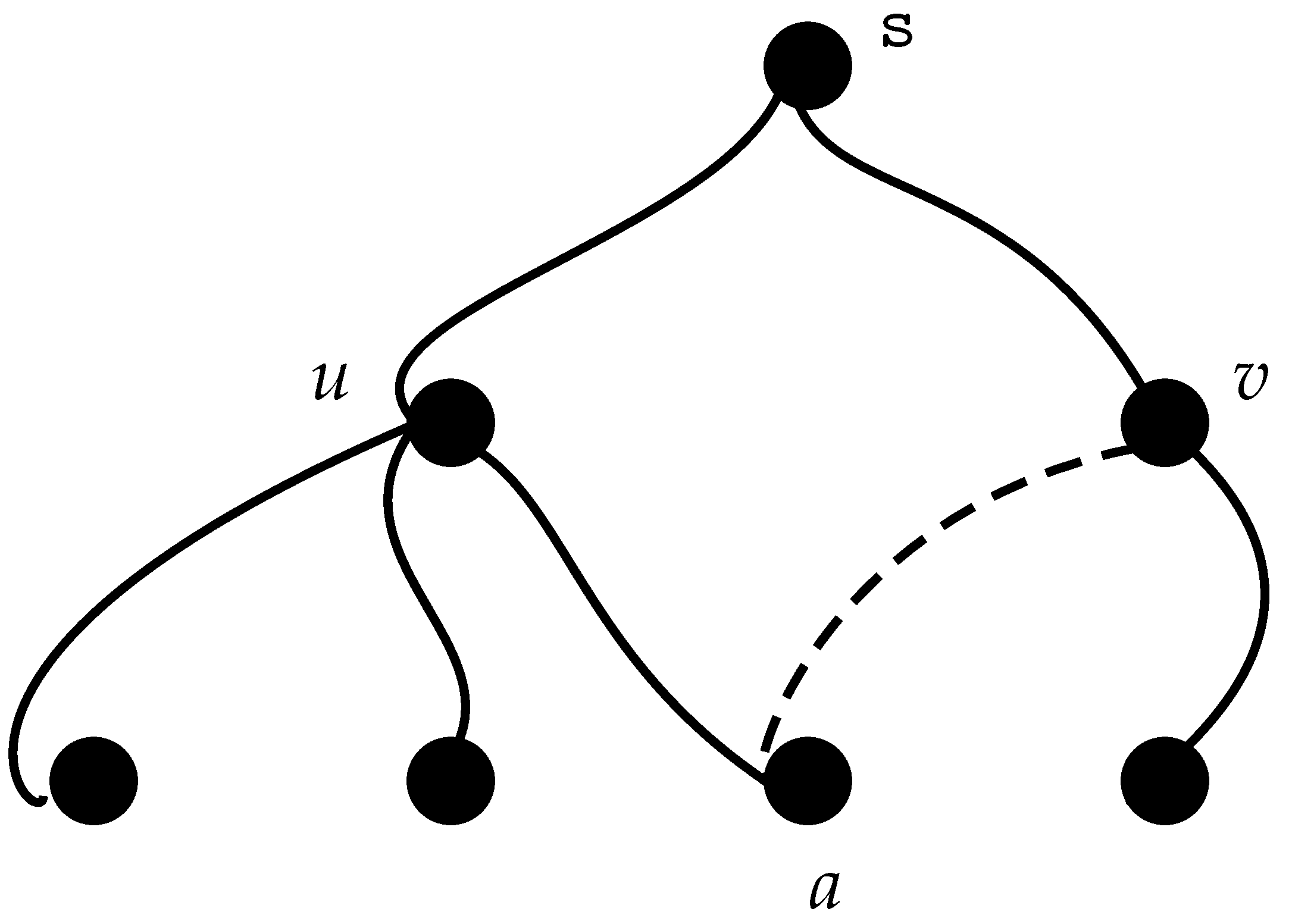
In this section, the parameters that affect the operation of the considered wireless sensor network are given.

3.1. Topology Model

A connected undirected graph G ( V , E ) represents the considered wireless sensor network, which was assumed to have a planar topology. V signifies the set of nodes, while E defines the set of links among the network nodes. n is the network size, and n = | V | . If a link ( u , v ) exists between two network nodes u and v, i.e., ( u , v ) E , then node u and node v are referred to as neighbors, and a transmission event can occur directly between them. Let h ( u , v ) represent the number of links (or hops) between nodes u and v along the shortest path connecting them. As a result, h ( u , v ) = 1 if ( u , v ) i n E . Allow the Euclidean distance χ ( u , v ) for a link ( u , v ) to match the link’s weight. This weight is proportional to the amount of energy used to transmit data over this particular link; the greater the Euclidean distance, the more energy is spent. It should be noted however that the amount of energy consumed per transmission was considered to be the same for all nodes in this study. The latter assumption is a typical one because nodes are frequently considered to consume the maximum amount of transmission power for each transmission (see, for example, [26]).

3.2. The Sink Node

s is the sink node, a network node that represents the specific network node that has been selected to be in charge of gathering all sensed information from the wireless sensor network. In other words, all data packets created by every node in the network have to be delivered to the sink node. As is commonly stated in the literature, the sink node is supposed to be connected to some type of infrastructure that provides appropriate connectivity, as well as an abundant source of energy.
In has to be noted that there is a substantial difference between this work and the majority of the rest of the literature, and it is based on the network node that is assumed to serve the role of the sink node. The sink node is typically referred to as an extra node in most works of the literature, yet in most circumstances, it has more capabilities than the other nodes (e.g., in [27] and other works, it is supposed that it can travel and collect data from other nodes). On the other hand, the term “sink” in the current paper is supposed to be a network feature that can be implemented on one of the existing, conventional network nodes, already deployed to a location in the field before the proposed technique is applied or the network starts operating. The selection of the sink node is expected to take place just after the initial placement of the nodes has been completed.
When the sink is held by a node (or placed on a node) u, then u takes on the role of the sink node or u is a node that holds the sink. The sink node is chosen from among the nodes that have previously been (uniformly) deployed in the network; it is designated by the letter s and is expected to be connected to some infrastructure that provides plentiful power supply to the network. In this sense, s is excluded from the energy consumption study, as well as it cannot play the role of the most energy-consuming node.

3.3. Routing Model

Routing enables data packet relaying among neighbor nodes in order to reach the sink node s , which is the case for all sensor data created by any network node. This work does not provide any routing technique, but it aimed at making use of the results of any already implemented routing technique on the network by applying the algorithm after considering the initial routing results. In this sense, a simple shortest path approach was employed here. Unlike the theoretical approach, which assumes that the weight of a connection ( u , v ) is equal to one for all links, the simulations took into account the distance in hops h ( u , s ) to find the shortest path between a node u and a sink node s . After the shortest path is implemented and before the appliance of the proposed algorithm, a node u is notified about its parent node p u s , which is actually the next hop (from u) for a data packet to reach s for all data packets originated or forwarded by node u.

3.4. Traffic Load Model

The traffic load model here is based on the data packets that have to be transmitted by a node in a time step during the network operation, as given in [24]. The number of data packets a node carries and needs to be transmitted not only contains the packets that the node creates itself, but the those created by other nodes and that need to be forwarded towards the sink node as well [23,28].
Suppose a node v has just received a data packet generated by another node u; in this case, node v is responsible for forwarding the data packet towards the sink node s , along with any other data packets generated by node v. Let l u signify the average number of data packets generated by a node u in each time step, which is referred to as the traffic load of node u. Suppose that L s ( u ) represents the cumulative traffic load of node u when the sink node is s . The cumulative traffic load L s ( u ) is actually the sum of the traffic loads of all nodes whose packets travel through node u in order to reach the sink node, and it is represented by the expression
L s ( u ) = v T s ( u ) l v
where T s ( u ) denotes a sub-tree (its root being node u) of the shortest path tree (created by the routing model) rooted at the sink node.

3.5. Energy Model

All nodes, with the exception of the sink node s , are considered to be in a state of idle mode during the very first time step of the network’s operation, i.e., at the very beginning of the network’s activity. Nodes in idle mode are waiting to be triggered by a sensing operation. A sensing operation takes place when a node either gathers a metric using its own sensors or receives a data packet containing data sensed by another node and needs to be forwarded towards the sink node. Let ϵ u s ( t ) signify the amount of energy left in node u’s battery at time instance t when the sink node is s . It was assumed that all nodes are completely charged at the beginning of the network’s operation, i.e., when t = 0 . In this sense, given a node u and a sink node s , the expression
ϵ u s ( 0 ) = ϵ max
satisfies the condition for u V , where ϵ max is referred to as the battery’s capacity. During the initial stages of the network’s operation, it was supposed that the battery capacity of all nodes is the same.
By the time a node is triggered, either a sensing operation is about to begin or a data packet has been received and needs to be forwarded towards the sink node. Following the sensing and processing steps, the data are forwarded to the sink node through the shortest path tree in both circumstances. When a transmission from node u to node v takes place, it is assumed that the energy level of the node u battery will be lowered by the amount of transmission energy, denoted by the symbol e .
Taking the above into consideration and in conjunction with Equation (1), it can be assumed that at every time step t, the average energy consumed (or the energy consumption by a node u) when the sink node is node s , denoted by β s ( u ) , is as follows:
β s ( u ) = L s ( u ) e

4. The Proposed Algorithm

In this section, the most energy-consuming node idea is described, along with the proposed algorithm. The primary goal set here was to minimize the energy consumption of the most energy-consuming node, thus prolonging the network’s lifetime. The secondary goal was achieving a more balanced cumulative traffic load allocation, in terms of fairness among the network nodes.

4.1. The Most Energy-Consuming Node

As the failure of a node operating at any time instance could be a significant disadvantage for the network to fulfill its goals, the considered network in this work is supposed to end its operation when any of its nodes depletes its battery. As already mentioned, the sink node is supposed to hold an abundant energy supply; thus, the focus is on the energy consumption of the rest of the network nodes. As a result, the goal is to identify this particular (non-sink) node that will deplete its battery first and, therefore, be responsible for the network termination. Let T denote the time instance at which the network termination occurs.
It can be assumed that the node that consumes the most, in terms of energy consumption, will be the one that will make the network terminate. Let κ be the specific node that will cause the network’s termination, that is the node that holds the highest energy consumption value among the network nodes in the network. Given Equation (3) and n network nodes, it holds that
β s ( κ ) = max 0 u n 1 β s ( u ) .
Given that the energy consumption e for transmission in the considered wireless sensor network is assumed to be the same for all transmissions taking place from any network node, then node κ , the node that is responsible for the network’s termination, is also the node holding the highest value on its cumulative traffic load L s ( u ) .
In many circumstances, the shortest path approach will produce pathways to the sink node that pass through some nodes more frequently than other nodes on the way to the sink. Since some nodes are closer to the sink node than the other nodes, this is an acceptable outcome; nevertheless, it also results in an energy hole problem [29]. Because of the energy hole problem and the fact that nodes adjacent to the sink node must relay a substantial amount of traffic load, their energy consumption is higher than that of other, more distant from the sink node, nodes in the same network configuration. One of these high-energy-consumption nodes, κ , is the one that will cause a network termination.
Considering a node u as the most energy-consuming node, then u = κ . Note that the focus here is not limited to decreasing the energy consumption of κ , which is u in this case. In some cases, the assignment of more than one parent to the nodes may result in a different node holding the maximum value of energy consumption. The algorithm is targeted at minimizing the value of the maximum energy consumption held among nodes, not at minimizing the energy consumption of the node that has been calculated to be κ . This is significant to take into account, as minimizing the energy consumption of κ alone could result in a different node holding more energy consumption than κ ’s initial value. This part of the paper’s goals is further explained in the next subsection, along with an example illustrating the above statement and the usage of the proposed algorithm.

4.2. The Proposed Algorithm’s Approach

Given a sink node s , the suggested algorithm’s purpose is to reduce the energy consumption of the resulting most energy-consuming node κ for the selected sink node s in order to extend the network’s lifespan to its maximum potential. Given Equation (3), it can be inferred that lowering the cumulative traffic load of κ , as determined by L s ( κ ) , will result in a reduction in the energy consumption of the most energy-consuming node. Moreover, keeping a balance among all nodes’ cumulative traffic load will ensure that obtaining a higher κ energy consumption as a result is minimized. Taking into consideration Equations (3) and (4), it can be inferred that reducing the maximum value of β s ( κ ) will result in a later battery depletion and, consequently, a later network termination.
This algorithm is meant to be used for nodes in a wireless sensor network that have been arbitrarily placed and after a routing technique has already provided its results. In order to accomplish the aforementioned goal, the suggested algorithm makes use of the findings of a straightforward shortest path technique. As a result, every node is assumed to be informed about the “identity” of its parent and the distance in hops between the parent and the sink node. Then, the algorithm attempts to determine whether there are any nodes that could have more than one parent, all of which have to be located at the same distance in hops from the sink node with the parent that was firstly allocated by the shortest path strategy. If such parents exist, the cumulative traffic load will be equally distributed among the parents who are located at the same distance from the sink node (which is also the initial parent’s distance from the sink node), which includes the parent who is the shortest path result’s parent. For example, when the algorithm has been executed, packets from a node with two parents will be relayed to both parents in the same manner.
For example, consider the simple network depicted in Figure 1. The lines correspond to the links among nodes, while the dashed line is an unused link after the shortest path algorithm is applied. Assuming equal traffic load for all nodes, l y = 1 , y V ( G ) , it is clear that the initial selection of paths will result in L s ( u ) = 4 and L s ( v ) = 2 ; the most energy-consuming node will be u ( L s ( u ) = 4 ); thus, κ = u. Applying the proposed algorithm will result in enabling link ( a , v ) and assigning a second parent to node a. Now, as a transmits half of its packets towards v, L s ( u ) = 3.5 and L s ( v ) = 2.5 , thus minimizing the cumulative traffic load of κ . As a result, the energy consumption of κ will also be less and the network lifetime will become higher than before applying the algorithm.
The steps followed by the proposed algorithm can be summarized as follows:
  • Select all nodes that are more than one hop away from the sink node s .
  • Find if any of the above nodes has one or more neighbors that hold the same distance in hops from the sink node with the initially allocated (by the simple shortest path approach) parent.
  • For nodes where (ii.) applies, assign all these neighbors as their parents.
  • During the wireless sensor network operation, the nodes will interchangeably use all their parents as the next step of their transmitted packets towards the sink node.
The proposed algorithm is shown in detail in Algorithm 1.
Algorithm 1 The Proposed Algorithm.
1:
procedureProposed-Algorithm( u [ n ] , n )▹ The procedure that goes through all network nodes n
2:
  for  j 0 to n 1 do                     ▹ For all network nodes
3:
   if  u [ j ] . h o p s > 1 then   ▹ Check if node u [ j ] is neither the sink node, nor is one hop away from the sink node
4:
      i n i t i a l P a r e n t H o p s = u [ j ] . i n i t i a l P a r e n t . h o p s  ▹ Declarations of a neighbor’s distance to become a parent
5:
      p a r e n t s [ ] = a s s i g n P a r e n t s ( u [ j ] , i n i t i a l P a r e n t H o p s )  ▹ Obtain the neighbors of distance equal to the initial parent’s one
6:
   end if
7:
  end for
8:
  return  p a r e n t s [ ]
9:
end procedure
10:
procedureassignParents( v , h o p s ) ▹ The procedure that returns the neighbors of a node v, of a distance equal to the initial parent’s one ( h o p s )
11:
p a r e n t s [ ] = 0                             ▹ Initialization
12:
for  i 0 to v . n u m O f N e i g h s do              ▹ For all node v’s neighbors
13:
   if  v . n e i g h [ i ] . h o p s F r o m S i n k = h o p s   then  ▹ If there are neighbors of a distance equal to the initial
14:
       p a r e n t s [ ] v . n e i g h [ i ]                    ▹ Use them as parents
15:
   end if
16:
end for
17:
return  p a r e n t s [ ]
18:
end procedure

5. Simulation Results

To enhance the analysis of the current work and evaluate the proposed algorithm, simulation scenarios were implemented using the OMNeT++ simulator [30]. In all cases, the sink node was assumed to be equipped with constantly recharged batteries; thus, the sink node’s energy consumption was not considered in the simulations. The network’s parameters and their corresponding values are depicted in Table 1. Note that, to achieve a more realistic approach, energy is consumed not only for transmitting packets, but for receiving packets, as well.

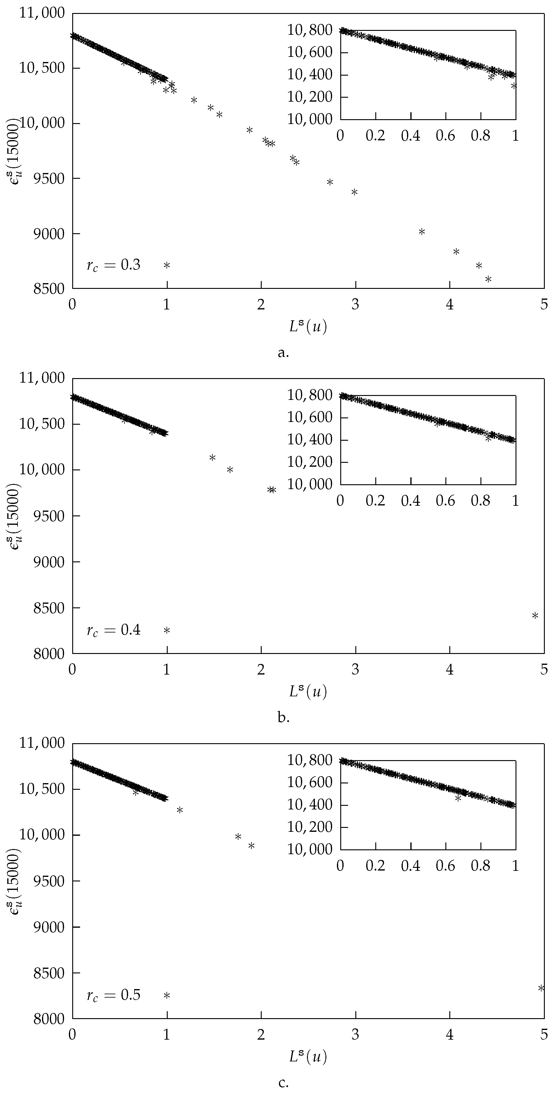
5.1. Energy Consumption vs. Cumulative Traffic Load

As the proposed algorithm’s operation mainly affects the cumulative traffic load of the network nodes and in order to have a better view of the impact of the proposed algorithm, it is helpful to, first, study the connection of the cumulative traffic load to the nodes’ energy consumption. In Figure 2, the residual energy of all network nodes at t = 15,000 is depicted against the value of their cumulative traffic load (resulting from the simple shortest path approach) for three values of the connectivity radius, denoted by r c . The time instance value (i.e., t = 15,000) is selected based on the termination time of the network (i.e., three networks based on the three values of r c ) that terminated first. It is shown in this figure that the higher the cumulative traffic load of a node, the less its residual energy is; thus, the node whose cumulative traffic load holds the largest value will also be the node that will terminate first.

5.2. The Proposed Algorithm Evaluation

In this subsection, the effects of the proposed algorithm on the cumulative traffic load of the network nodes are given in order to show how the algorithm minimizes its values and how it results in a fairer cumulative traffic load distribution among nodes. Moreover, the termination time is studied here to show the effects of the proposed algorithm on it.

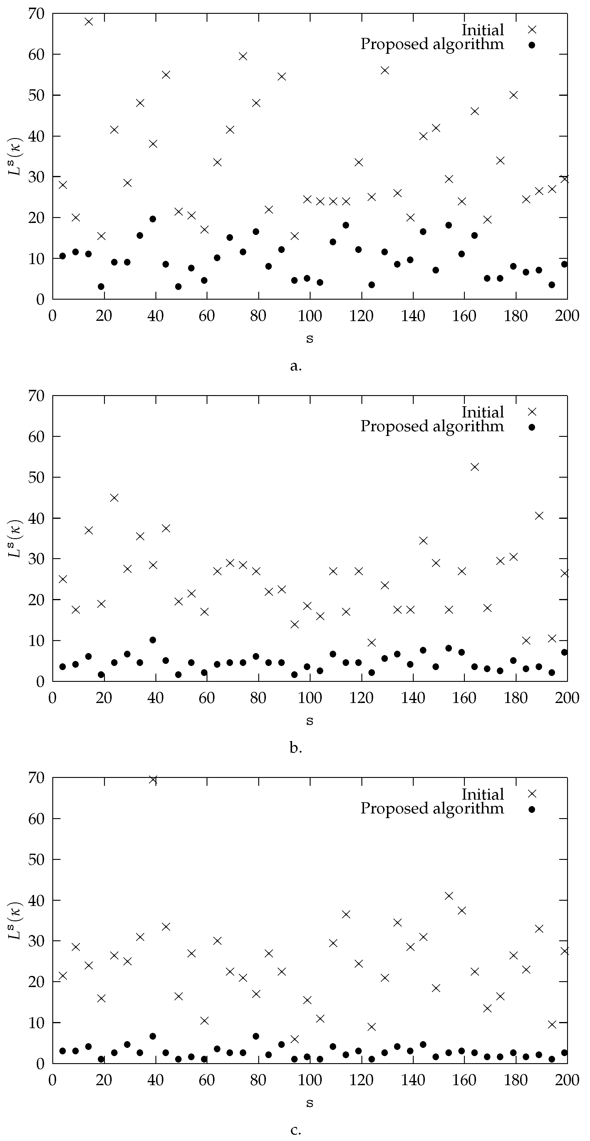
5.2.1. Algorithm’s Effects on Cumulative Traffic Load

In order to have a clearer view of the algorithm’s effects on the cumulative traffic load, Figure 3 shows the impact of the proposed algorithm on the cumulative traffic load of the most energy-consuming node of the network. More specifically, the initial (i.e., before applying the algorithm) cumulative traffic load of the most energy-consuming node is depicted, along with the resulting cumulative traffic load after the algorithm’s application. Note that for better visualization, the results depicted concern the average of every five values (e.g., s = 4 shows the average initial and resulting cumulative traffic load for s = 0 …4). It is shown here that for all values of s , the cumulative traffic load of the most energy-consuming node is always less when the proposed algorithm is applied.

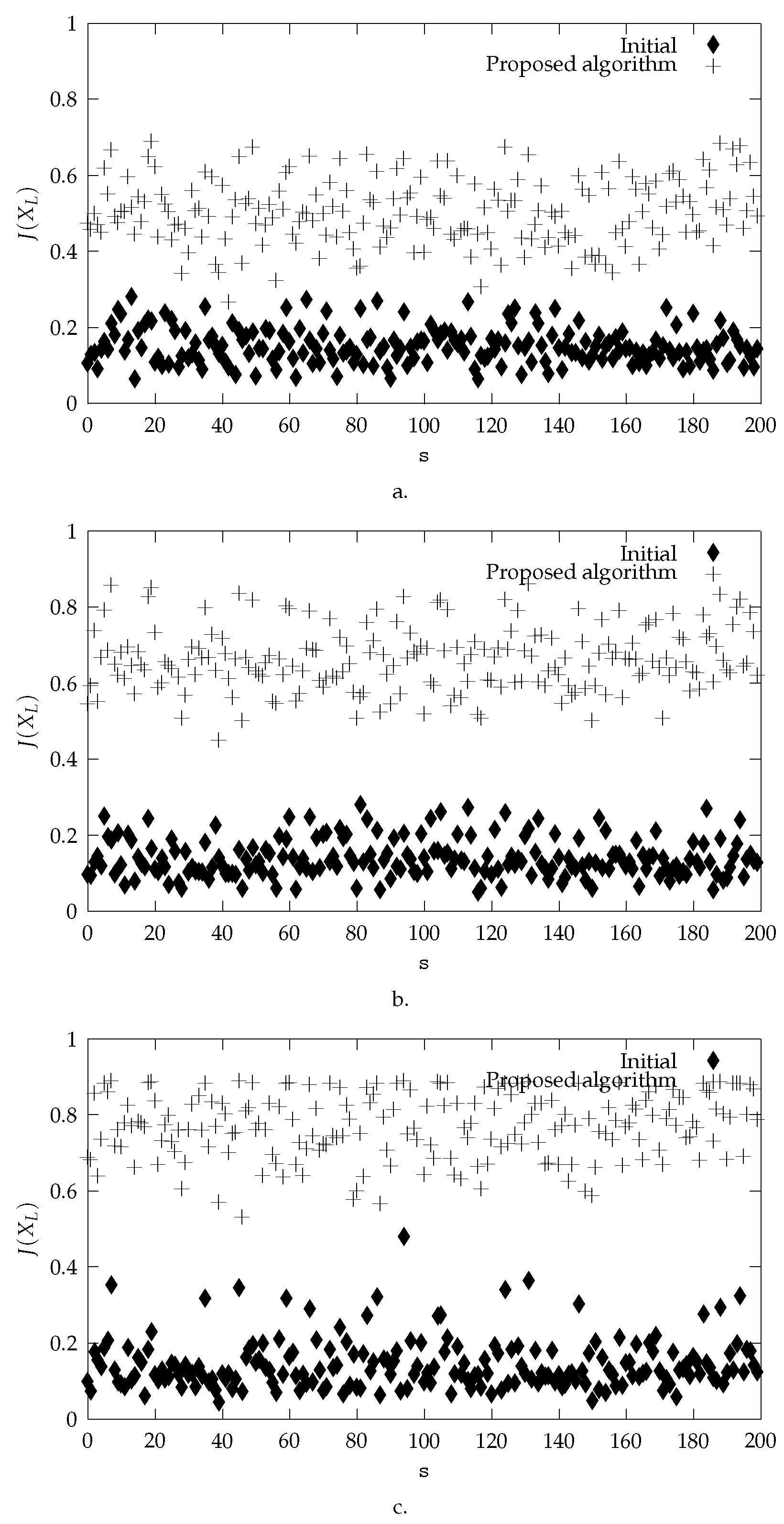
5.2.2. Fairness Results

Among the numerous fairness metrics [31], Jain’s index [25] was considered in this work as the tool to measure the fairness resulting from the proposed algorithm and compare it against the fairness of the initial cumulative traffic load allocation that resulted from the shortest path approach explained earlier. Jain’s index provides a simple centralized way of evaluating a system’s fairness. It is defined as
J ( X L ) = [ L L u ] 2 n L L u 2
where L u is node u’s resource allocation, the cumulative traffic load in this paper’s case, and X L is a vector of all nodes’ cumulative traffic loads. The previous function produces a value within the [0, …, 1] range. The higher this value, the fairer the system is. When J ( X L ) is close to 0, this indicates that the vast majority of individuals are mistreated in favor of a few. In contrast, when resources are allocated evenly among the individuals, it is the case that J ( X L ) = 1 .
In Figure 4, the resulting Jain index J ( X L ) difference between the initial parents’ selection and the one resulting from the proposed algorithm is depicted for all possible selections of sink node s (i.e., each symbol represents a different simulation) and three different values of r c ( r c = 0.3 , r c = 0.4 , and r c = 0.5 ). It is shown here that, in all cases, applying the algorithm resulted in a fairer cumulative traffic load allocation among the network nodes.

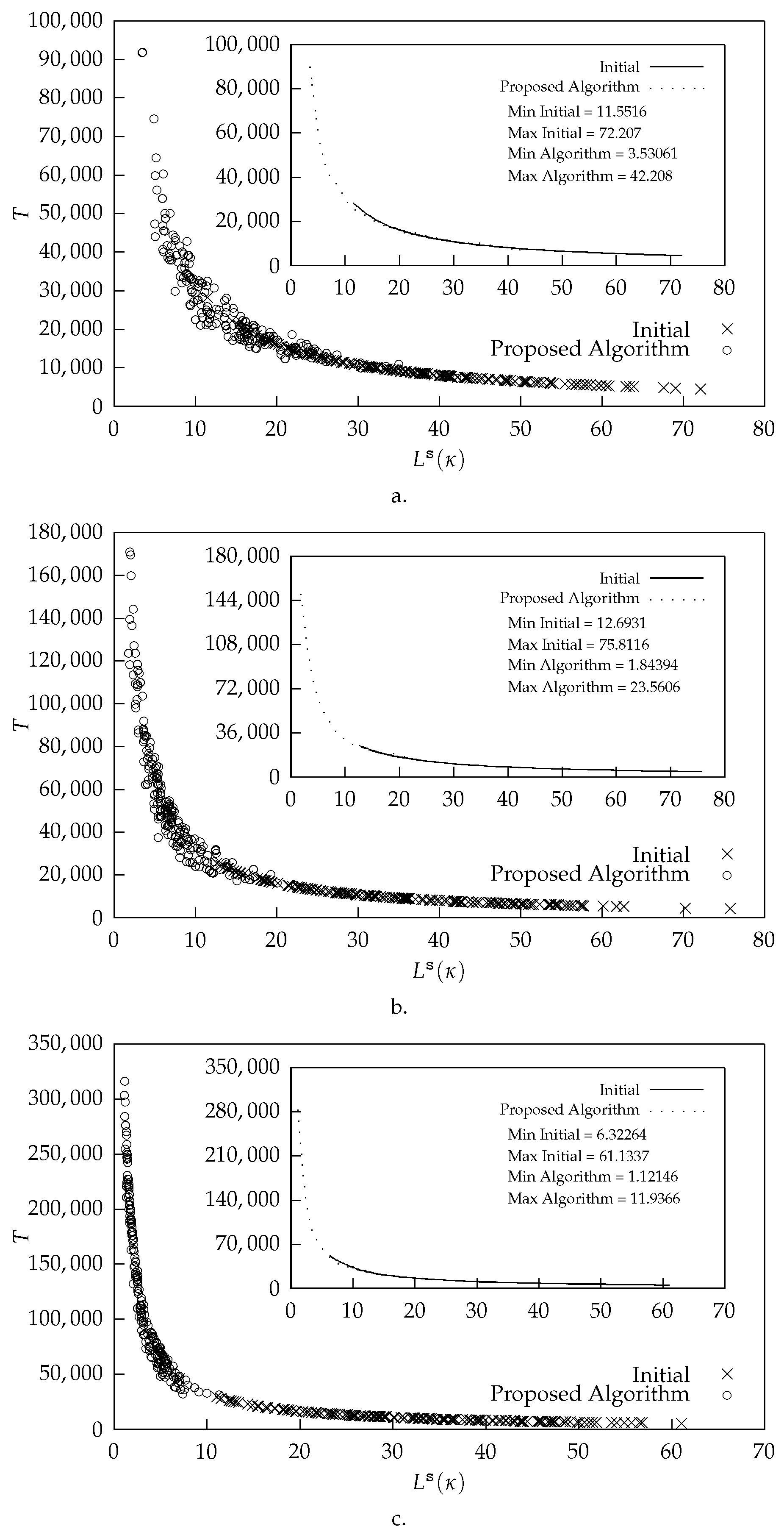
5.2.3. Termination Time Results

Keeping in mind that the network will be terminated when the node with the highest cumulative traffic load depletes its battery, the performance of the proposed algorithm is further tested in the sequel. According to the description given in Section 4, the algorithm’s purpose is to reduce the cumulative traffic load on the most energy-consuming node κ in order to extend the network’s lifetime. In Figure 5, the values of termination time T are plotted against the cumulative traffic load of the most energy-consuming node L s ( κ ) when each node plays the role of the sink node (i.e., each dot represents a different simulation) and three different values of r c (i.e., r c = 0.3 , r c = 0.4 , and r c = 0.5 ). It is shown here that when the proposed algorithm was applied, the network lifetime was lengthened for all three values of r c . Both situations (i.e., the initial case and the case after the algorithm application) had their own minimum and maximum values given, demonstrating that the minimum and maximum values of T were always minimized following the application of the proposed method.

6. Conclusions

This study showed that the energy consumption of a wireless sensor network node vastly depends on the total amount of traffic carried by it. Taking into account that the energy hole problem results in increased energy consumption for nodes closer to the sink node, one of these close-to-the-sink nodes will be the one that will transmit the most and the one that will terminate the network operation at the same time. In this sense, a traffic-load-based algorithm was proposed in this paper in order to reduce the energy consumption of the most energy-consuming node and extend, in this way, the total lifetime of the network. The suggested algorithm takes advantage (i.e., knowledge about parent assignment and distance in hops) of the results of the shortest path approach that is applied prior to the algorithm’s usage and is independent of the proposed algorithm (i.e., any shortest path approach that provides parent assignment can be exploited by the proposed algorithm). Then, for all nodes, the proposed algorithm discovers the neighbors that are within the same distance (in hops) from the sink node with the parent that was initially assigned by the shortest path approach. If such neighbors can be identified, they are all used as parents, and the traffic load is distributed among them in an equal and equitable manner. The proposed algorithm was evaluated under the simulation results. The results showed that the algorithm met the objectives set, hence extending the network’s lifespan and achieving a more equitable (fairer) traffic load distribution among network nodes. Future work will be focused on mathematically modeling the investigated problem, along with the limitations accompanying it. For example, the role the connectivity radius plays in finding more than one parent for a node is inevitably significant. Moreover, in order to further show the effectiveness of the proposed algorithm, more results have to be considered related to other metrics, such as reliable packet delivery.

Author Contributions

Conceptualization, G.T. and C.T.A.; methodology, G.T. and K.K.; software, G.T. and N.G.; validation, N.G., A.T.T. and E.G.; formal analysis, A.T.T.; investigation, E.G.; resources, K.K.; data curation, E.K. and K.K.; writing—original draft preparation, G.T.; writing—review and editing, K.B.; visualization, E.K.; supervision, C.T.A. All authors have read and agreed to the published version of the manuscript.

Funding

This research received no external funding.

Institutional Review Board Statement

Not applicable.

Informed Consent Statement

Not applicable.

Data Availability Statement

Not applicable.

Conflicts of Interest

The authors declare no conflict of interest.

Appendix A

Table A1. Notations.
h ( u , v ) Distance in hops between nodes u and v
s Sink node
p u s Parent node of node u when the sink node is s
l u Traffic load of node u
L s ( u ) Cumulative traffic load of node u when the sink node is s
e Energy consumed by a network node for the transmission of a packet
β s ( u ) Average energy consumption of node u
κ Network node with the maximum average energy consumption
ϵ u s ( t ) Residual energy of node u at time instance t
TTermination time
ϵ max Battery capacity
r c Connectivity radius

References

  1. Akyildiz, I.F.; Su, W.; Sankarasubramaniam, Y.; Cayirci, E. Wireless sensor networks: A survey. Comput. Netw. 2002, 38, 393–422. [Google Scholar] [CrossRef] [Green Version]
  2. Akyildiz, I.F.; Melodia, T.; Chowdhury, K.R. A survey on wireless multimedia sensor networks. Comput. Netw. 2007, 51, 921–960. [Google Scholar] [CrossRef]
  3. Anastasi, G.; Conti, M.; Di Francesco, M.; Passarella, A. Energy conservation in wireless sensor networks: A survey. Ad Hoc Netw. 2009, 7, 537–568. [Google Scholar] [CrossRef]
  4. Ogundile, O.O.; Alfa, A.S. A survey on an energy-efficient and energy-balanced routing protocol for wireless sensor networks. Sensors 2017, 17, 1084. [Google Scholar] [CrossRef] [Green Version]
  5. Arjunan, S.; Pothula, S. A survey on unequal clustering protocols in wireless sensor networks. J. King Saud Univ. Comput. Inf. Sci. 2019, 31, 304–317. [Google Scholar] [CrossRef]
  6. Jan, B.; Farman, H.; Javed, H.; Montrucchio, B.; Khan, M.; Ali, S. Energy efficient hierarchical clustering approaches in wireless sensor networks: A survey. Wirel. Commun. Mob. Comput. 2017, 2017, 6457942. [Google Scholar] [CrossRef] [Green Version]
  7. Randhawa, S.; Jain, S. MLBC: Multi-objective load balancing clustering technique in wireless sensor networks. Appl. Soft Comput. 2019, 74, 66–89. [Google Scholar] [CrossRef]
  8. Edla, D.R.; Kongara, M.C.; Cheruku, R. SCE-PSO based clustering approach for load balancing of gateways in wireless sensor networks. Wirel. Netw. 2019, 25, 1067–1081. [Google Scholar] [CrossRef]
  9. Sampathkumar, A.; Mulerikkal, J.; Sivaram, M. Glowworm swarm optimization for effectual load balancing and routing strategies in wireless sensor networks. Wirel. Netw. 2020, 26, 4227–4238. [Google Scholar] [CrossRef]
  10. Krishnanand, K.; Ghose, D. Glowworm swarm optimisation: A new method for optimising multi-modal functions. Int. J. Comput. Intell. Stud. 2009, 1, 93–119. [Google Scholar] [CrossRef]
  11. Tabibi, S.; Ghaffari, A. Energy-efficient routing mechanism for mobile sink in wireless sensor networks using particle swarm optimization algorithm. Wirel. Pers. Commun. 2019, 104, 199–216. [Google Scholar] [CrossRef]
  12. Kacimi, R.; Dhaou, R.; Beylot, A.L. Load balancing techniques for lifetime maximizing in wireless sensor networks. Ad Hoc Netw. 2013, 11, 2172–2186. [Google Scholar] [CrossRef] [Green Version]
  13. Dorigo, M.; Stützle, T. Ant colony optimization: Overview and recent advances. Handb. Metaheuristics 2019, 311–351. [Google Scholar] [CrossRef] [Green Version]
  14. Li, X.; Keegan, B.; Mtenzi, F.; Weise, T.; Tan, M. Energy-efficient load balancing ant based routing algorithm for wireless sensor networks. IEEE Access 2019, 7, 113182–113196. [Google Scholar] [CrossRef]
  15. Lipare, A.; Edla, D.R.; Kuppili, V. Energy efficient load balancing approach for avoiding energy hole problem in WSN using Grey Wolf Optimizer with novel fitness function. Appl. Soft Comput. 2019, 84, 105706. [Google Scholar] [CrossRef]
  16. Sharma, K.P.; Sharma, T.P. Energy-hole avoidance and lifetime enhancement of a WSN through load factor. Turk. J. Electr. Eng. Comput. Sci. 2017, 25, 1375–1387. [Google Scholar] [CrossRef]
  17. Jan, N.; Javaid, N.; Javaid, Q.; Alrajeh, N.; Alam, M.; Khan, Z.A.; Niaz, I.A. A balanced energy-consuming and hole-alleviating algorithm for wireless sensor networks. IEEE Access 2017, 5, 6134–6150. [Google Scholar] [CrossRef]
  18. Kumar, S.; Gautam, P.R.; Verma, A.; Verma, R.; Kumar, A. Energy Efficient Routing using Sectors Based Energy-Hole Reduction in WSNs. In Proceedings of the 2019 International Conference on Electrical, Electronics and Computer Engineering (UPCON), Aligarh, India, 8–10 November 2019; IEEE: Piscataway, NJ, USA, 2019; pp. 1–4. [Google Scholar]
  19. Kushal, B.; Chitra, M. Cluster based routing protocol to prolong network lifetime through mobile sink in WSN. In Proceedings of the 2016 IEEE International Conference on Recent Trends in Electronics, Information & Communication Technology (RTEICT), Bangalore, India, 20–21 May 2016; IEEE: Piscataway, NJ, USA, 2016; pp. 1287–1291. [Google Scholar]
  20. Khan, Z.A.; Awais, M.; Alghamdi, T.A.; Khalid, A.; Fatima, A.; Akbar, M.; Javaid, N. Region Aware Proactive Routing Approaches Exploiting Energy Efficient Paths for Void Hole Avoidance in Underwater WSNs. IEEE Access 2019, 7, 140703–140722. [Google Scholar] [CrossRef]
  21. Krishnamoorthy, A.; Vijayarajan, V. Energy aware routing technique based on Markov model in wireless sensor network. Int. J. Comput. Appl. 2020, 42, 23–29. [Google Scholar] [CrossRef]
  22. Zhang, J.; Lin, Z.; Tsai, P.W.; Xu, L. Entropy-driven data aggregation method for energy-efficient wireless sensor networks. Inf. Fusion 2020, 56, 103–113. [Google Scholar] [CrossRef]
  23. Tsoumanis, G.; Oikonomou, K.; Koufoudakis, G.; Aissa, S. Energy-efficient sink placement in wireless sensor networks. Comput. Netw. 2018, 141, 166–178. [Google Scholar] [CrossRef]
  24. Tsoumanis, G.; Oikonomou, K.; Aïssa, S.; Stavrakakis, I. Energy and Distance Optimization in Rechargeable Wireless Sensor Networks. IEEE Trans. Green Commun. Netw. 2020, 5, 378–391. [Google Scholar] [CrossRef]
  25. Jain, R.K.; Chiu, D.M.W.; Hawe, W.R. A Quantitative Measure of Fairness and Discrimination; Eastern Research Laboratory, Digital Equipment Corporation: Hudson, MA, USA, 1984. [Google Scholar]
  26. Madan, R.; Lall, S. Distributed algorithms for maximum lifetime routing in wireless sensor networks. IEEE Trans. Wirel. Commun. 2006, 5, 2185–2193. [Google Scholar] [CrossRef]
  27. Thomson, C.; Wadhaj, I.; Tan, Z.; Al-Dubai, A. Towards an energy balancing solution for wireless sensor network with mobile sink node. Comput. Commun. 2021, 170, 50–64. [Google Scholar] [CrossRef]
  28. Tsoumanis, G.; Oikonomou, K.; Aïssa, S.; Stavrakakis, I. A recharging distance analysis for wireless sensor networks. Ad Hoc Netw. 2018, 75, 80–86. [Google Scholar] [CrossRef] [Green Version]
  29. Li, J.; Mohapatra, P. Analytical modeling and mitigation techniques for the energy hole problem in sensor networks. Pervasive Mob. Comput. 2007, 3, 233–254. [Google Scholar] [CrossRef]
  30. Varga, A. OMNeT++. In Modeling and Tools for Network Simulation; Springer: Berlin/Heidelberg, Germany, 2010; pp. 35–59. [Google Scholar]
  31. Huaizhou, S.; Prasad, R.V.; Onur, E.; Niemegeers, I. Fairness in wireless networks: Issues, measures and challenges. IEEE Commun. Surv. Tutor. 2013, 16, 5–24. [Google Scholar] [CrossRef]
Figure 1. A simple network.
Information 13 00202 g001
Figure 2. Residual energy of all network nodes at t = 15,000, over the cumulative traffic load L s ( u ) , for three values of r c ((a) r c = 0.3 , (b) r c = 0.4 , and (c) r c = 0.5 ).
Information 13 00202 g002
Figure 3. Cumulative traffic load of the most energy-consuming node L s ( κ ) before (initial) and after applying the algorithm (proposed algorithm), for each sink node s and three different values of r c ((a) r c = 0.3 , (b) r c = 0.4 , and (c) r c = 0.5 ).
Information 13 00202 g003
Figure 4. Jain index J ( X L ) before (initial) and after applying the algorithm (proposed algorithm), for each sink node s and three different values of r c ((a) r c = 0.3 , (b) r c = 0.4 , and (c) r c = 0.5 ).
Information 13 00202 g004
Figure 5. Termination time T against the cumulative traffic load of the most energy-consuming node L s ( κ ) before (initial) and after (proposed algorithm) applying the algorithm when each node plays the role of the sink node, for three different values of r c ((a) r c = 0.3 , (b) r c = 0.4 , and (c) r c = 0.5 ).
Information 13 00202 g005
Table 1. Simulation Network Parameters.
ParameterValue
Network area[0 m, 1000 m] × [0 m, 1000 m]
Number of nodes n200
Traffic load l u 0.5
Nodes’ initial energy ϵ M a x ( u ) 10,800 J
Processing energy0.1 J
Transmitter current27 mA
Receiver current10 mA
Packet length1024 B
Data rate4.8 kBps
Voltage3 V
Publisher’s Note: MDPI stays neutral with regard to jurisdictional claims in published maps and institutional affiliations.

