
Model-Based Underwater Image Simulation and Learning-Based Underwater Image Enhancement Method

Abstract
:1. Introduction
- We propose a sophisticated underwater image simulation and selection method for generating training sets for learning-based underwater image enhancement methods. To the best of our knowledge, the proposed method covers a wider range of degradation problems than previous methods and is the first one that can simulate underwater images with uneven lighting and generate training sets specialized for the targeted real-world images.
- We propose an efficient CNN to learn the translation from degraded underwater images to clear enhanced images. Owing to the smooth transmission of information in the proposed network, textures and structures of the original underwater images can be well-preserved in the enhanced images.
- The proposed method also outperforms many state-of-the-art methods, especially in enhancing underwater images with challenging degradation problems, such as strong light scattering or insufficient lighting.
2. Related Works
2.1. Methods Based on General Image Processing Skills
2.2. Methods Based on Physical Models
2.3. Methods Based on Deep Learning
3. Methodology of Underwater Image Simulation
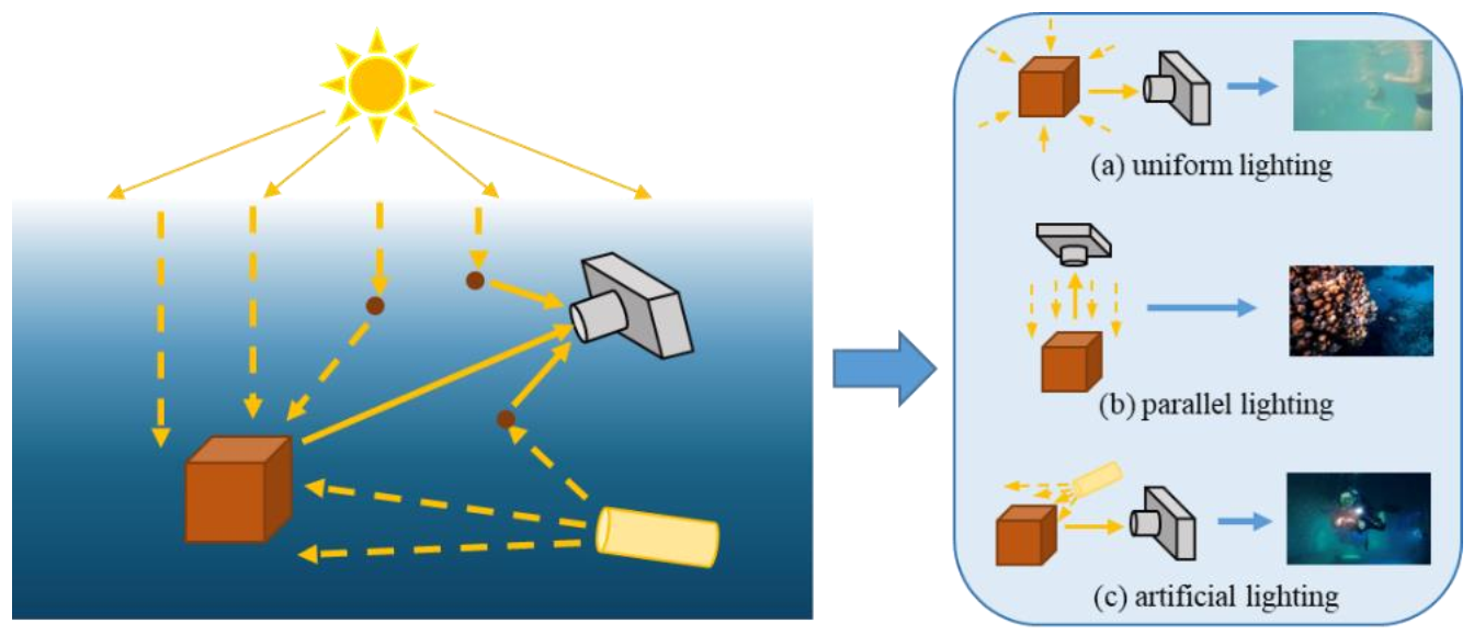
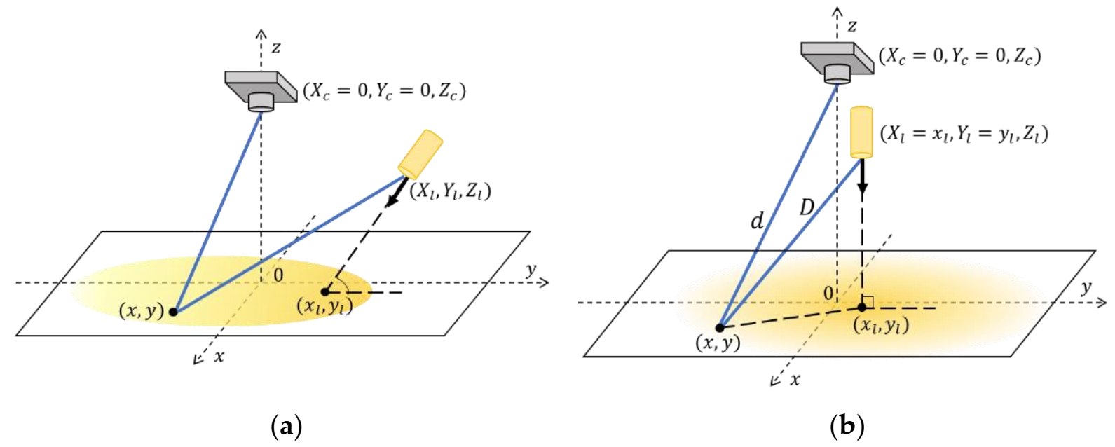
3.1. Proposed Underwater Image Degradation Model
3.2. Generating Reliable Training Sets by Underwater Image Simulation and Selection
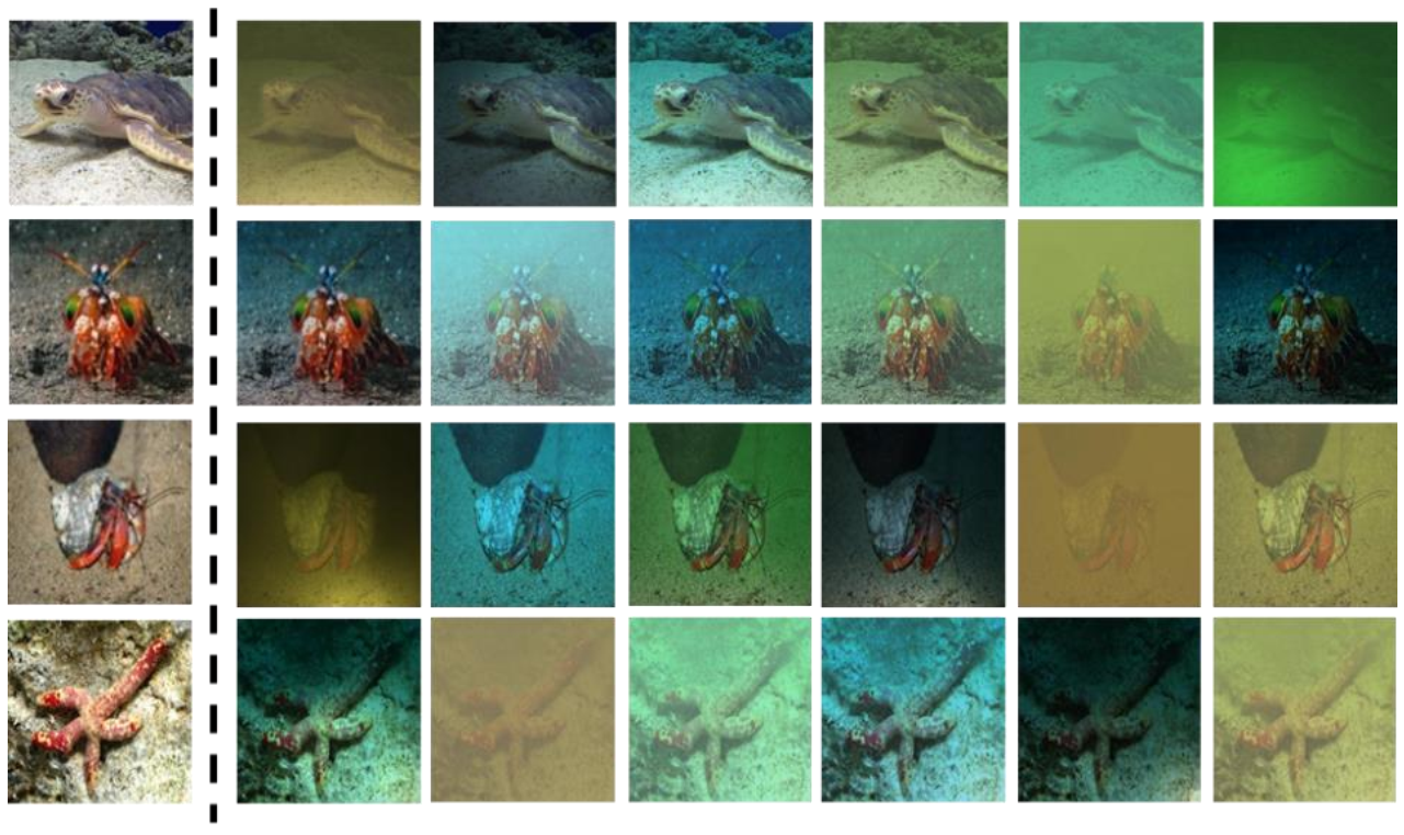
3.2.1. Underwater Image Simulation with Broadened Ranges of Parameter Values
- (1)
- Simulation of lighting parameters and
- (2)
- Parameter setting of channel-wise attenuation coefficients
- (3)
- Parameter setting of transmission distance
- (4)
- Parameter setting of κ
- (5)
- Generating underwater image
3.2.2. Generating Reliable Training Sets Based on Image Selection
- (1)
- Selecting simulated underwater images with similar color deviations as the targeted image sets
- (2)
- Selecting simulated underwater images with enough details preserved
4. A Modular CNN for Learning to Enhance Degraded Underwater Images
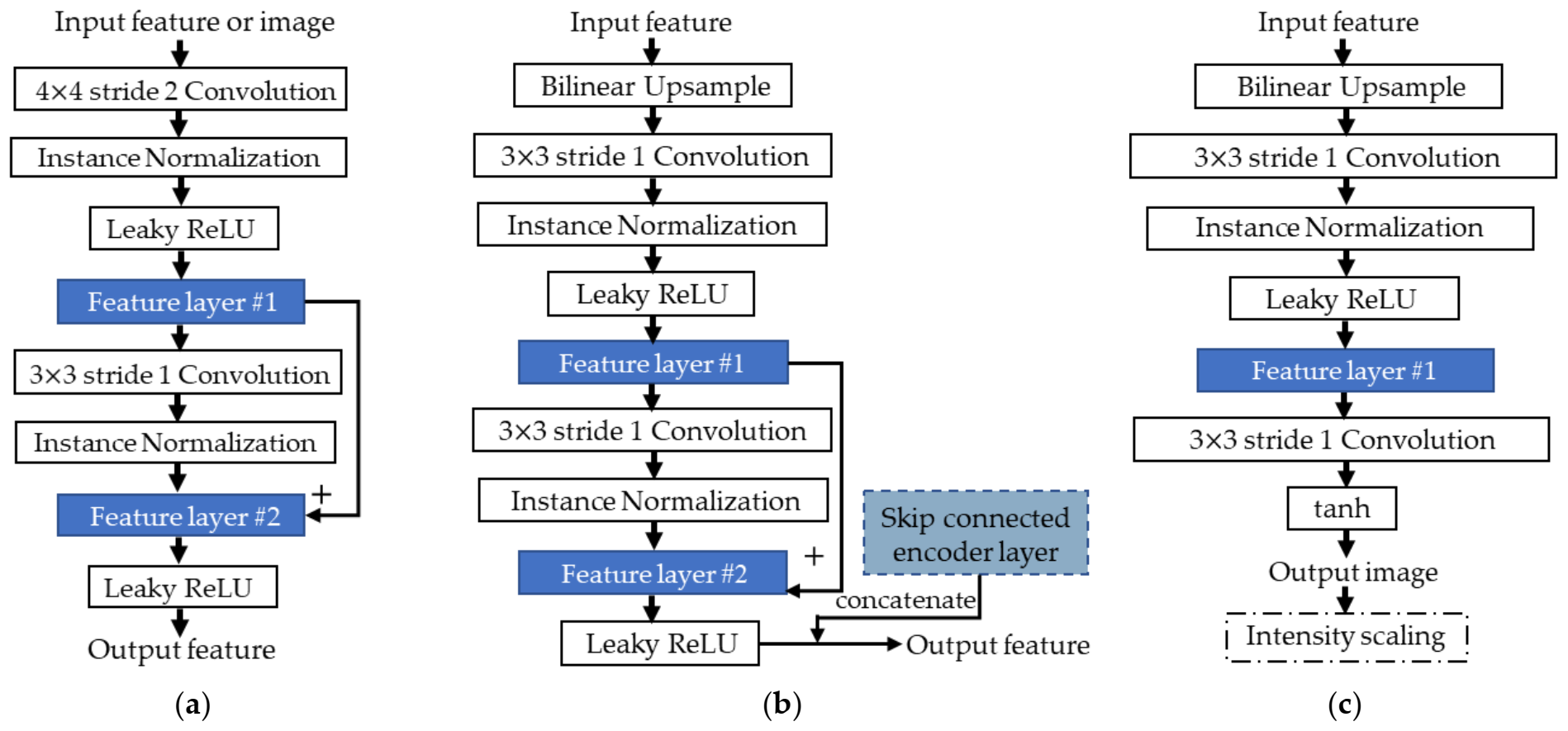
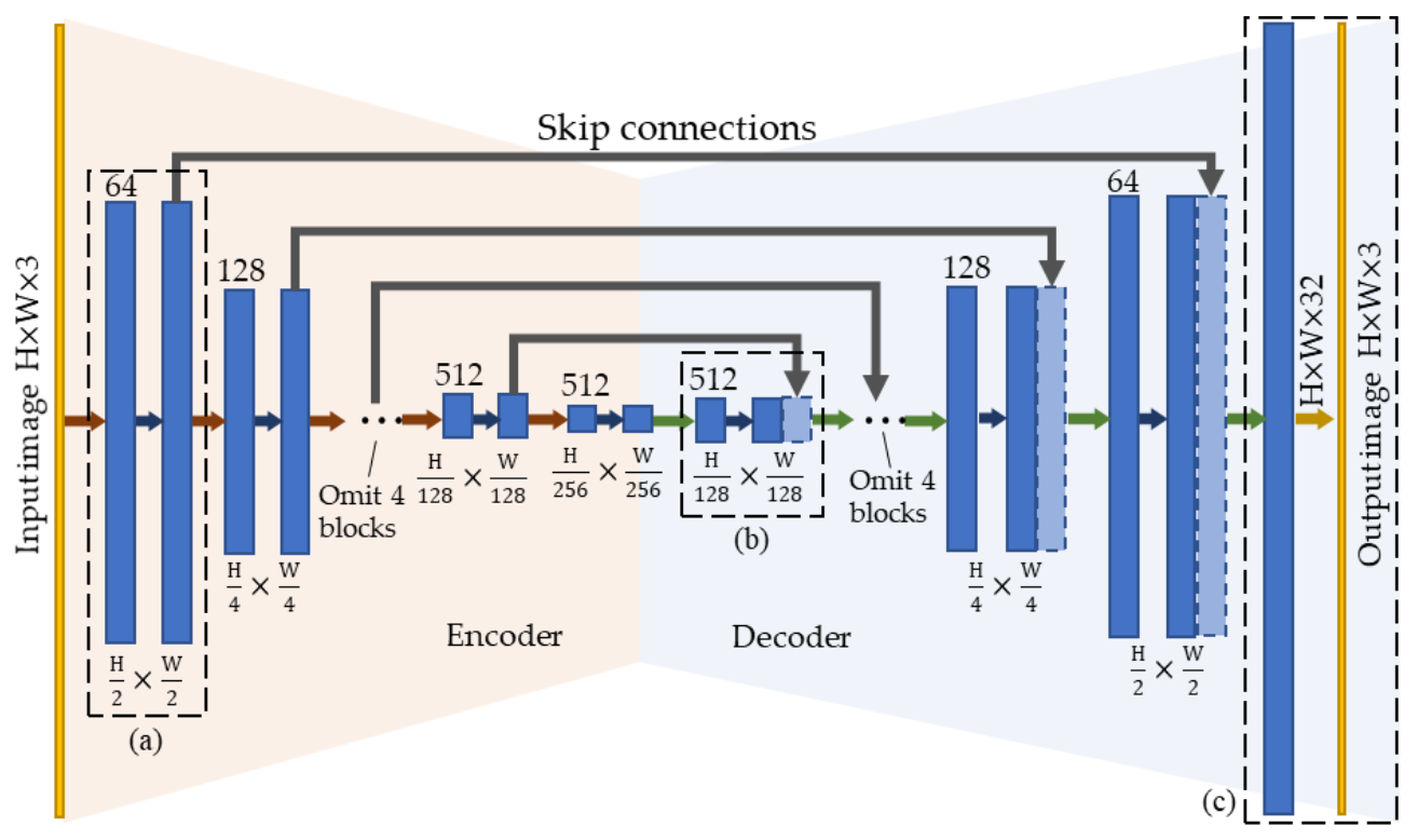
4.1. Network Architecture
4.2. Objective Function
5. Experimental Results
5.1. Evaluation on Simulated Underwater Images with Various Degradation Problems
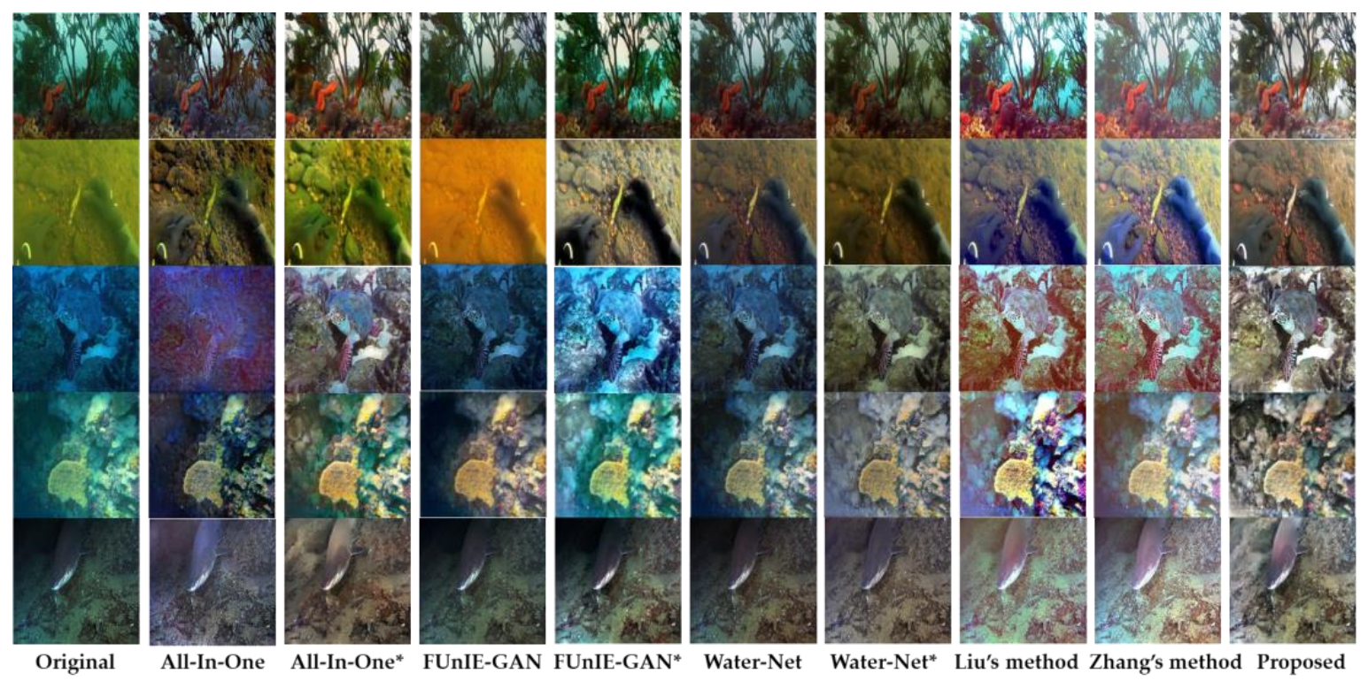
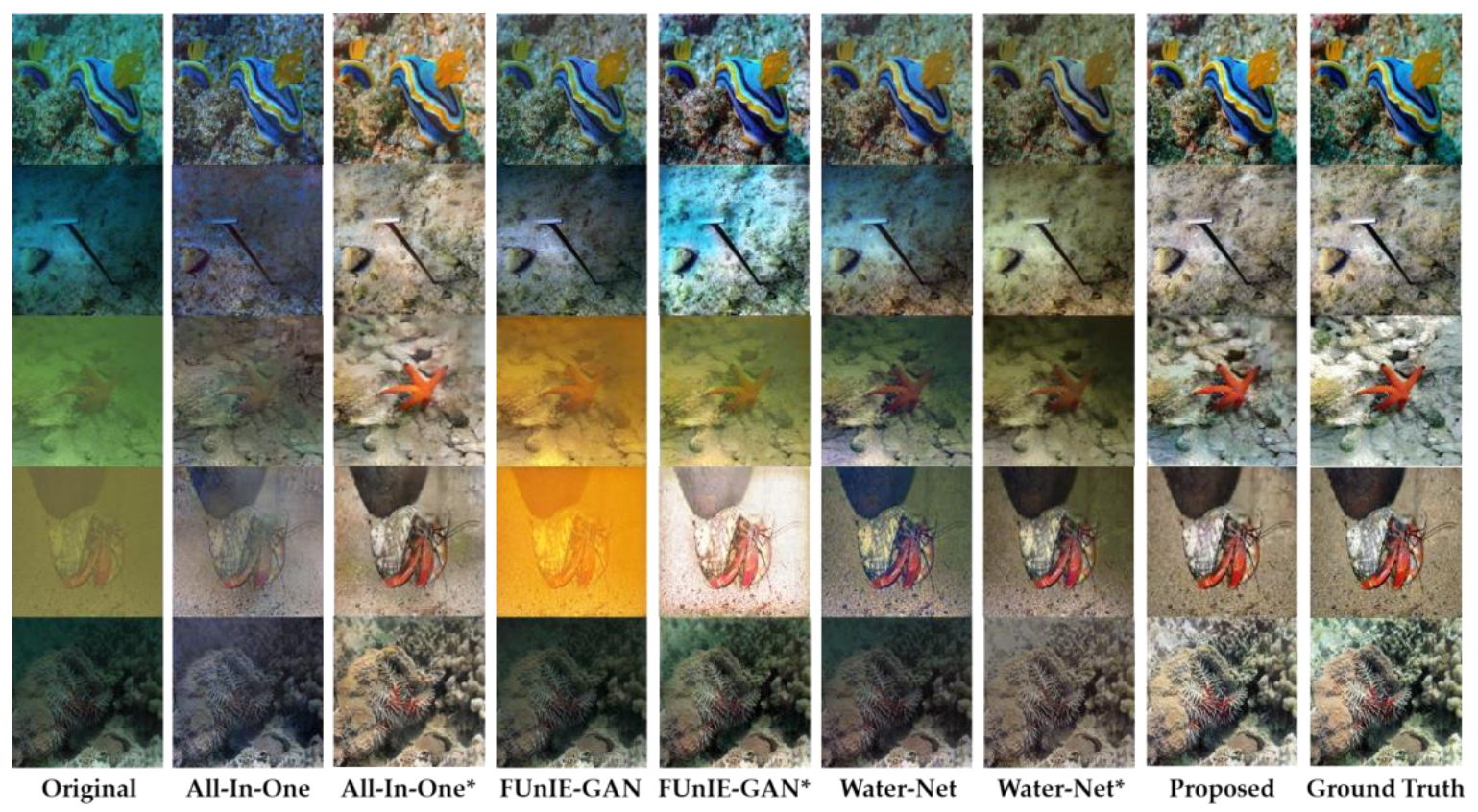
5.2. Evaluation on Real-World Underwater Images with Various Degradation Problems
6. Conclusions
Author Contributions
Funding
Institutional Review Board Statement
Informed Consent Statement
Data Availability Statement
Acknowledgments
Conflicts of Interest
References
- Chen, X.; Yang, Y.-H. A Closed-Form Solution to Single Underwater Camera Calibration Using Triple Wavelength Dispersion and Its Application to Single Camera 3D Reconstruction. IEEE Trans. Image Process. 2017, 26, 4553–4561. [Google Scholar] [CrossRef] [PubMed]
- Lu, H.; Uemura, T.; Wang, D.; Zhu, J.; Huang, Z.; Kim, H. Deep-Sea Organisms Tracking Using Dehazing and Deep Learning. Mob. Netw. Appl. 2018, 25, 1008–1015. [Google Scholar] [CrossRef]
- Agrafiotis, P.; Drakonakis, G.I.; Georgopoulos, A.; Skarlatos, D. The Effect of Underwater Imagery Radiometry on 3D Reconstruction and Orthoimagery. Int. Arch. Photogramm. Remote Sens. Spat. Inf. Sci. 2017, XLII-2/W3, 25–31. [Google Scholar] [CrossRef] [Green Version]
- Chuang, M.-C.; Hwang, J.-N.; Williams, K. A Feature Learning and Object Recognition Framework for Underwater Fish Images. IEEE Trans. Image Process. 2016, 25, 1862–1872. [Google Scholar] [CrossRef]
- Lee, D.; Kim, G.; Kim, D.; Myung, H.; Choi, H.-T. Vision-based object detection and tracking for autonomous navigation of underwater robots. Ocean Eng. 2012, 48, 59–68. [Google Scholar] [CrossRef]
- Wang, Y.; Song, W.; Fortino, G.; Qi, L.-Z.; Zhang, W.; Liotta, A. An Experimental-Based Review of Image Enhancement and Image Restoration Methods for Underwater Imaging. IEEE Access 2019, 7, 140233–140251. [Google Scholar] [CrossRef]
- Yang, M.; Hu, J.; Li, C.; Rohde, G.; Du, Y.; Hu, K. An In-Depth Survey of Underwater Image Enhancement and Restoration. IEEE Access 2019, 7, 123638–123657. [Google Scholar] [CrossRef]
- Forbes, T.; Goldsmith, M.; Mudur, S.; Poullis, C. DeepCaustics: Classification and Removal of Caustics from Underwater Imagery. IEEE J. Ocean. Eng. 2018, 44, 728–738. [Google Scholar] [CrossRef]
- Reggiannini, M.; Moroni, D. The Use of Saliency in Underwater Computer Vision: A Review. Remote Sens. 2020, 13, 22. [Google Scholar] [CrossRef]
- Islam, M.J.; Xia, Y.; Sattar, J. Fast Underwater Image Enhancement for Improved Visual Perception. IEEE Robot. Autom. Lett. 2020, 5, 3227–3234. [Google Scholar] [CrossRef] [Green Version]
- Li, C.; Anwar, S.; Porikli, F. Underwater scene prior inspired deep underwater image and video enhancement. Pattern Recognit. 2020, 98, 107038. [Google Scholar] [CrossRef]
- Li, C.; Guo, C.; Ren, W.; Cong, R.; Hou, J.; Kwong, S.; Tao, D. An Underwater Image Enhancement Benchmark Dataset and Beyond. IEEE Trans. Image Process. 2020, 29, 4376–4389. [Google Scholar] [CrossRef] [Green Version]
- Ronneberger, O.; Fischer, P.; Brox, T. U-Net: Convolutional networks for biomedical image segmentation. In Medical Image Computing and Computer-Assisted Intervention 2015; Navab, N., Hornegger, J., Wells, W.M., Frangi, A.F., Eds.; Springer International Publishing: Cham, Switzerland, 2015; pp. 234–241. [Google Scholar] [CrossRef] [Green Version]
- He, K.; Zhang, X.; Ren, S.; Sun, J. Deep residual learning for image recognition. In Proceedings of the 2016 IEEE Conference on Computer Vision and Pattern Recognition (CVPR), Las Vegas, NV, USA, 27–30 June 2016. [Google Scholar]
- Iqbal, K.; Salam, R.A.; Osman, A.; Talib, A.Z. Underwater Image Enhancement Using an Integrated Colour Model. IAENG Int. J. Comput. Sci. 2007, 32, 239–244. [Google Scholar]
- Ancuti, C.O.; Ancuti, C.; Haber, T.; Bekaert, P. Fusion-based restoration of the underwater images. In Proceedings of the 2011 18th IEEE International Conference on Image Processing, Brussels, Belgium, 11–14 September 2011; pp. 1557–1560. [Google Scholar] [CrossRef]
- Ancuti, C.O.; Ancuti, C.; De Vleeschouwer, C.; Bekaert, P. Color Balance and Fusion for Underwater Image Enhancement. IEEE Trans. Image Process. 2018, 27, 379–393. [Google Scholar] [CrossRef] [Green Version]
- Fu, X.; Zhuang, P.; Huang, Y.; Liao, Y.; Zhang, X.-P.; Ding, X. A retinex-based enhancing approach for single underwater image. In Proceedings of the 2014 IEEE International Conference on Image Processing (ICIP), Paris, France, 27–30 October 2014; pp. 4572–4576. [Google Scholar] [CrossRef]
- Zhang, W.; Li, G.; Ying, Z. A new underwater image enhancing method via color correction and illumination adjustment. In Proceedings of the 2017 IEEE Visual Communications and Image Processing (VCIP), St. Petersburg, FL, USA, 10–13 December 2017; pp. 1–4. [Google Scholar] [CrossRef]
- Peng, Y.-T.; Cosman, P. Underwater Image Restoration Based on Image Blurriness and Light Absorption. IEEE Trans. Image Process. 2017, 26, 1579–1594. [Google Scholar] [CrossRef]
- He, K.; Sun, J.; Tang, X. Single Image Haze Removal Using Dark Channel Prior. IEEE Trans. Pattern Anal. Mach. Intell. 2011, 33, 2341–2353. [Google Scholar] [CrossRef]
- Galdran, A.; Pardo, D.; Picon, A.; Alvarez-Gila, A. Automatic Red-Channel underwater image restoration. J. Vis. Commun. Image Represent. 2015, 26, 132–145. [Google Scholar] [CrossRef] [Green Version]
- Drews, P., Jr.; do Nascimento, E.; Moraes, F.; Botelho, S.; Campos, M. Transmission Estimation in Underwater Single Images. In Proceedings of the 2013 IEEE International Conference on Computer Vision Workshops, Sydney, Australia, 2–8 December 2013; pp. 825–830. [Google Scholar] [CrossRef]
- Carlevaris-Bianco, N.; Mohan, A.; Eustice, R.M. Initial results in underwater single image dehazing. In Proceedings of the OCEANS 2010 MTS/IEEE SEATTLE, Seattle, WA, USA, 20–23 September 2010; pp. 1–8. [Google Scholar]
- Liu, Y.; Xu, H.; Shang, D.; Li, C.; Quan, X. An Underwater Image Enhancement Method for Different Illumination Conditions Based on Color Tone Correction and Fusion-Based Descattering. Sensors 2019, 19, 5567. [Google Scholar] [CrossRef] [Green Version]
- Marques, T.P.; Albu, A.B.; Hoeberechts, M. A Contrast-Guided Approach for the Enhancement of Low-Lighting Underwater Images. J. Imaging 2019, 5, 79. [Google Scholar] [CrossRef] [Green Version]
- Uplavikar, P.; Wu, Z.; Wang, Z. All-In-One Underwater Image Enhancement using Domain-Adversarial Learning. arXiv 2019, arXiv:1905.13342. [Google Scholar]
- Wang, N.; Zhou, Y.; Han, F.; Zhu, H.; Zheng, Y. UWGAN: Underwater GAN for Real-world Underwater Color Restoration and Dehazing. arXiv 2019, arXiv:1912.10269. [Google Scholar]
- Li, J.; Skinner, K.A.; Eustice, R.M.; Johnson-Roberson, M. WaterGAN: Unsupervised generative network to enable real-time color correction of monocular underwater images. IEEE Robot. Autom. Lett. 2017, 3, 387–394. [Google Scholar] [CrossRef] [Green Version]
- Li, C.; Anwar, S.; Hou, J.; Cong, R.; Guo, C.; Ren, W. Underwater Image Enhancement via Medium Transmission-Guided Multi-Color Space Embedding. IEEE Trans. Image Process. 2021, 30, 4985–5000. [Google Scholar] [CrossRef]
- Fabbri, C.; Islam, J.; Sattar, J. Enhancing Underwater Imagery Using Generative Adversarial Networks. In Proceedings of the 2018 IEEE International Conference on Robotics and Automation (ICRA), Brisbane, Australia, 21–25 May 2018; pp. 7159–7165. [Google Scholar] [CrossRef] [Green Version]
- Zhu, J.-Y.; Park, T.; Isola, P.; Efros, A.A. Unpaired image-to-image translation using cycle-consistent adversarial networks. In Proceedings of the IEEE International Conference on Computer Vision, Venice, Italy, 22–29 October 2017; pp. 2223–2232. [Google Scholar]
- Guo, Y.; Li, H.; Zhuang, P. Underwater Image Enhancement Using a Multiscale Dense Generative Adversarial Network. IEEE J. Ocean. Eng. 2020, 45, 862–870. [Google Scholar] [CrossRef]
- Liu, X.; Gao, Z.; Chen, B.M. MLFcGAN: Multilevel Feature Fusion-Based Conditional GAN for Underwater Image Color Correction. IEEE Geosci. Remote Sens. Lett. 2019, 17, 1488–1492. [Google Scholar] [CrossRef] [Green Version]
- Jaffe, J. Computer modeling and the design of optimal underwater imaging systems. IEEE J. Ocean. Eng. 1990, 15, 101–111. [Google Scholar] [CrossRef]
- McGlamery, B.L. A Computer Model for Underwater Camera Systems. SPIE Proc. 1980, 208, 221–231. [Google Scholar] [CrossRef]
- Schechner, Y.; Karpel, N. Clear underwater vision. In Proceedings of the 2004 IEEE Computer Society Conference on Computer Vision and Pattern Recognition, 2004. CVPR 2004, Washington, DC, USA, 27 June–2 July 2004; Volume 1, pp. 536–543. [Google Scholar] [CrossRef] [Green Version]
- Schechner, Y.Y.; Karpel, N. Recovery of Underwater Visibility and Structure by Polarization Analysis. IEEE J. Ocean. Eng. 2005, 30, 570–587. [Google Scholar] [CrossRef] [Green Version]
- Akkaynak, D.; Treibitz, T.; Shlesinger, T.; Loya, Y.; Tamir, R.; Iluz, D. What is the Space of Attenuation Coefficients in Underwater Computer Vision? In Proceedings of the 2017 IEEE Conference on Computer Vision and Pattern Recognition (CVPR), Honolulu, HI, USA, 21–26 July 2017; pp. 568–577. [Google Scholar]
- Zhao, X.; Jin, T.; Qu, S. Deriving inherent optical properties from background color and underwater image enhancement. Ocean Eng. 2015, 94, 163–172. [Google Scholar] [CrossRef]
- Mobley, C.D. Light and Water: Radiattive Transfer in Natural Waters; Academic Press: New York, NY, USA, 1994. [Google Scholar]
- Li, Z.; Snavely, N. MegaDepth: Learning Single-View Depth Prediction from Internet Photos. In Proceedings of the 2018 IEEE/CVF Conference on Computer Vision and Pattern Recognition, Salt Lake City, UT, USA, 18–23 June 2018; pp. 2041–2050. [Google Scholar]
- Ulyanov, D.; Vedaldi, A.; Lempitsky, V. Instance Normalization: The Missing Ingredient for Fast Stylization. arXiv 2016, arXiv:1607.08022. [Google Scholar]
- Maas, A.L.; Hannun, A.Y.; Ng, A.Y. Rectifier nonlinearities improve neural network acoustic models. In Proceedings of the 30th ICML Workshop on Deep Learning for Audio, Speech and Language Processing, Atlanta, GA, USA, 16–21 June 2013; Volume 28. [Google Scholar]
- Zhao, H.; Gallo, O.; Frosio, I.; Kautz, J. Loss Functions for Image Restoration with Neural Networks. IEEE Trans. Comput. Imaging 2017, 3, 47–57. [Google Scholar] [CrossRef]
- Lin, T.-Y.; Maire, M.; Belongie, S.; Hays, J.; Perona, P.; Ramanan, D.; Dollár, P.; Zitnick, C.L. Microsoft COCO: Common Objects in Context. In European Conference on Computer Vision, Proceedings of the 13th European Conference, Zurich, Switzerland, 6–12 September 2014; Springer: Cham, Switzerland, 2014; Volume 8693, pp. 740–755. [Google Scholar]
- Yang, M.; Sowmya, A. An Underwater Color Image Quality Evaluation Metric. IEEE Trans. Image Process. 2015, 24, 6062–6071. [Google Scholar] [CrossRef] [PubMed]
- Panetta, K.; Gao, C.; Agaian, S. Human-Visual-System-Inspired Underwater Image Quality Measures. IEEE J. Ocean. Eng. 2016, 41, 541–551. [Google Scholar] [CrossRef]
- Li, F.; Wu, J.; Wang, Y.; Zhao, Y.; Zhang, X. A color cast detection algorithm of robust performance. In Proceedings of the 2012 IEEE Fifth International Conference on Advanced Computational Intelligence (ICACI), Nanjing, China, 18–20 October 2012; pp. 662–664. [Google Scholar]


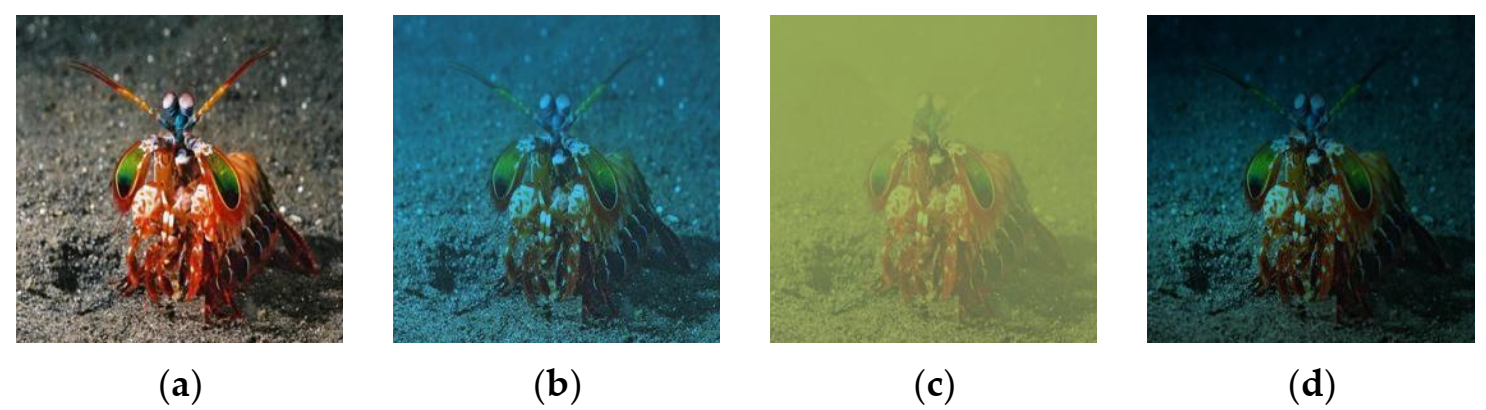
| Real-World Underwater Images | Simulated Underwater Images | |||||||
|---|---|---|---|---|---|---|---|---|
| Images |  |  |  |  |  |  |  | 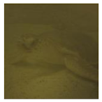 |
| Color tones |  |  |  |  |  |  |  |  |
| HSVs | [185, 0.54, 0.56] | [151, 0.45, 0.33] | [61, 0.37, 0.50] | [75, 0.85, 0.28] | [172, 0.40, 0.50] | [150, 0.57, 0.48] | [48, 0.29, 0.62] | [48, 0.57, 0.35] |
| Clear Image | Simulated Underwater Images | |||||
|---|---|---|---|---|---|---|
| Images | 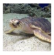 | 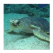 | 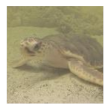 |  |  |  |
| Sobel-edge maps |  | 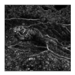 |  |  | 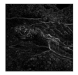 | 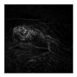 |
| NMADs | - | 0.34 | 0.59 | 0.93 | 0.62 | 0.78 |
| Group | Targeted Image Samples | Real-World Clear Images | Simulated Images after Selection |
|---|---|---|---|
| Set-A | 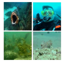 |  | 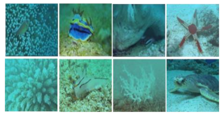 |
| Set-B |  |  | 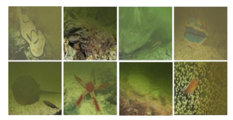 |
| Set-C |  |  |  |
| MSE↓ | PSNR↑ | SSIM↑ | Time (ms) | |
|---|---|---|---|---|
| Original | 0.0217 | 16.6390 | 0.5343 | - |
| All-In-One | 0.0170 | 17.7063 | 0.6543 | 13.9641 |
| All-In-One* | 0.0053 | 22.7201 | 0.8050 | - |
| FUnIE-GAN | 0.0266 | 15.7483 | 0.5671 | 7.5361 |
| FUnIE-GAN* | 0.0211 | 16.7601 | 0.6969 | - |
| Water-Net | 0.0180 | 17.4526 | 0.6913 | 80.4657 |
| Water-Net* | 0.0176 | 17.5337 | 0.6894 | - |
| Proposed | 0.0029 | 25.4209 | 0.8616 | 27.7387 |
| Color Deviation↓ | Edge Intensity↑ | Information Content↑ | |
|---|---|---|---|
| Original | 2.9042 | 0.1286 | 6.8242 |
| All-In-One | 1.5917 | 0.1941 | 6.9834 |
| All-In-One* | 1.2218 | 0.1965 | 7.2118 |
| FUnIE-GAN | 2.4229 | 0.1502 | 7.1567 |
| FUnIE-GAN* | 1.3253 | 0.2380 | 7.3171 |
| Water-Net | 0.8520 | 0.1603 | 7.2225 |
| Water-Net* | 1.0476 | 0.1701 | 7.0262 |
| Liu’s method | 0.4312 | 0.2593 | 7.3229 |
| Zhang’s method | 0.1132 | 0.2456 | 7.4529 |
| Proposed | 0.2988 | 0.2664 | 7.5247 |
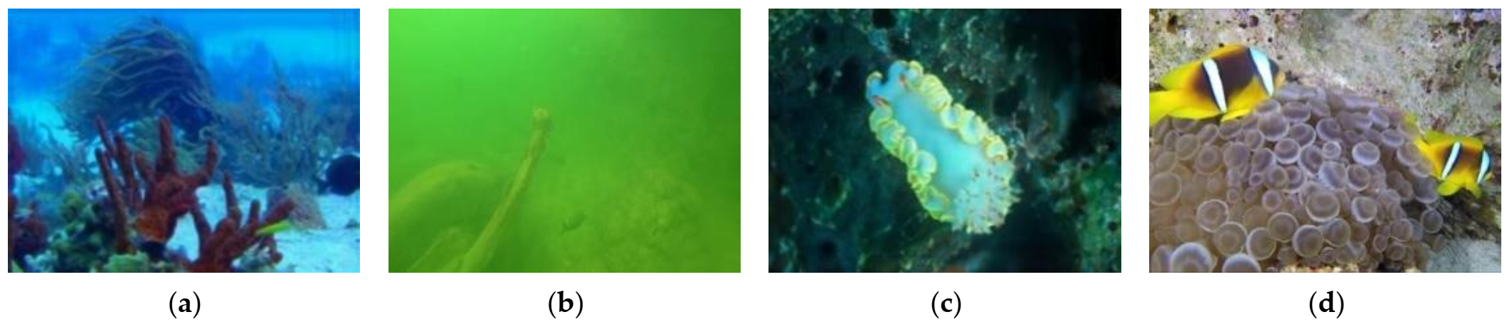
| Image | UICM↑ | UISM↑ | UIConM↑ | UIQM↑ | Edge Intensity↑ | Color Deviation↓ | Information Content↑ |
|---|---|---|---|---|---|---|---|
| Figure 10a | 6.1252 | 13.8233 | 0.2833 | 5.2677 | 0.1787 | 0.8622 | 7.2844 |
| Figure 10b | 3.6543 | 14.1887 | 0.2754 | 5.2775 | 0.1539 | 2.3381 | 7.1077 |
| Figure 10c | 0.8007 | 13.0062 | 0.2013 | 4.5832 | 0.0693 | 6.0097 | 6.2114 |
| Figure 10d | 3.6081 | 14.8173 | 0.1776 | 5.1124 | 0.1150 | 1.2231 | 6.4453 |
Publisher’s Note: MDPI stays neutral with regard to jurisdictional claims in published maps and institutional affiliations. |
© 2022 by the authors. Licensee MDPI, Basel, Switzerland. This article is an open access article distributed under the terms and conditions of the Creative Commons Attribution (CC BY) license (https://creativecommons.org/licenses/by/4.0/).
Share and Cite
Liu, Y.; Xu, H.; Zhang, B.; Sun, K.; Yang, J.; Li, B.; Li, C.; Quan, X. Model-Based Underwater Image Simulation and Learning-Based Underwater Image Enhancement Method. Information 2022, 13, 187. https://doi.org/10.3390/info13040187
Liu Y, Xu H, Zhang B, Sun K, Yang J, Li B, Li C, Quan X. Model-Based Underwater Image Simulation and Learning-Based Underwater Image Enhancement Method. Information. 2022; 13(4):187. https://doi.org/10.3390/info13040187
Chicago/Turabian StyleLiu, Yidan, Huiping Xu, Bing Zhang, Kelin Sun, Jingchuan Yang, Bo Li, Chen Li, and Xiangqian Quan. 2022. "Model-Based Underwater Image Simulation and Learning-Based Underwater Image Enhancement Method" Information 13, no. 4: 187. https://doi.org/10.3390/info13040187
APA StyleLiu, Y., Xu, H., Zhang, B., Sun, K., Yang, J., Li, B., Li, C., & Quan, X. (2022). Model-Based Underwater Image Simulation and Learning-Based Underwater Image Enhancement Method. Information, 13(4), 187. https://doi.org/10.3390/info13040187