Abstract
Due to the multi-technology advancements, internet of things (IoT) applications are in high demand to create smarter environments. Smart objects communicate by exchanging many messages, and this creates interference on receivers. Collection tree algorithms are applied to only reduce the nodes/paths’ interference but cannot fully handle the interference across the underlying IoT. This paper models and analyzes the interference spread in the IoT setting, where the collection tree routing algorithm is adopted. Node interference is treated as a real-life contamination of a disease, where individuals can migrate across compartments such as susceptible, attacked and replaced. The assumed typical collection tree routing model is the least interference beaconing algorithm (LIBA), and the dynamics of the interference spread is studied. The underlying network’s nodes are partitioned into groups of nodes which can affect each other and based on the partition property, the susceptible–attacked–replaced (SAR) model is proposed. To analyze the model, the system stability is studied, and the compartmental based trends are experimented in static, stochastic and predictive systems. The results shows that the dynamics of the system are dependent groups and all have points of convergence for static, stochastic and predictive systems.
1. Introduction
The world has entered in the era where intelligent machines have changed the production chain: the fourth industrial revolution (4IR) [1]. We are, additionally, in the era where the COVID-19 pandemic has geared the use of more advanced ways of digital communication. This has created high demand for the multi-technology, multi-protocol and multi-platform infrastructure, where IoT technologies play crucial roles.
It was discussed in [2] that the IoT is successful due to the fact that objects can now be manipulated daily to be outfitted with sensing, identification and positioning devices. The objects may be endowed with an internet protocol (IP) address to become smart objects, capable of communicating with not only other smart objects, but also with humans. In this case, it is expected to reach areas that we could not have reached without the advances made in sensing, identification and positioning technologies. While being globally discoverable and queried, these smart objects can similarly discover and interact with external entities by querying humans, computers and other smart objects [3].
The smart objects can also obtain intelligence by making or enabling context-related decisions by taking advantage of the available communication channels (see [4,5], for example) to provide information about themselves, and can access information that was aggregated by other smart objects [6]. The application domain for this technology may be found in many ways, including cyberphysical security [7], digital twins [8], surveillance [9], smart cities [10,11], smart transportation [12,13,14,15], smart buildings [16], smart energy [17], smart industry [18] and smart health [19]. These applications’ enabling technologies include sensor, nano-electronics, wireless sensor network (WSN) identification, localization, storage and cloud. However, IoT systems and applications are bound by security, privacy, safety, integrity, trust, dependability, transparency, anonymity and ethics constraints.
On the other hand, there has been several communication models in the IoT (see [20,21,22,23] for example) and in particular, the LIBA [24,25,26,27] has been proposed with the least interference beaconing paradigm as a frugal and lightweight IoT communication protocol. Here, the routing is done by a beaconing process that, as a result, produces a routing tree of the underlying network, which is rooted from the sink of the network. The routing is done by periodically sending beaconing messages in a network, and nodes communicate to form the tree routed at the sink. During the process, the path selection is done in such a way that the interference on nodes is minimized. The periodic repetition of the routing process enables nodes to change their paths to the sink and hence this is considered a collection tree algorithm and has been proven to be efficient in communication energy saving.
It is clear from [28] that in a real IoT deployment scenario, the very high interference values on nodes may be identified as an attack on the underlying IoT aiming at defeating the performance of the whole sensor network engineering mechanism. This could be done by influencing the routing processes and sending messages with wrong information about the nodes’ interference; this would lead to an incorrect routing tree. In this case, some nodes of the network would be overused while alternative ones remain underused. This would be considered an attack which may target, for example, the ventilation system of a power plant by messing up the weight of the mote that controls the temperature of the plant and thus congest that node by spamming it with traffic from other nodes. This might disable any communication between that node and the actuator that kicks off the air conditioning upon temperature changes. Communication security measures may be considered to mitigate this issue. However, there could be a scenario where, even if all communications are secured and a collection tree routing is correctly used, at a certain time, a node would have been sending and receiving a lot of messages to the point where it can no longer operate properly. Such nodes may be understood as nodes which have been subjected to a high level of interference, and this would inevitably affect other nodes in the same WSN.
Depending on the level of interference for each node of an IoT, nodes can clearly be grouped in compartments. The increase in interference of a node can lead to its migration from one compartment to another. This can, therefore, be compared with a normal human epidemic contamination, where an individual can move, for example, from a susceptible compartment to an attacked/infected compartment or to a replaced/diagnosed compartment, or even from an infected to diagnosed compartment. This kind of epidemic model can be achieved, in the case of WSN, by considering nodes with low interference levels as nodes in the susceptible compartment, being a sign of the less used nodes (nodes which have sent few messages and can still send many more); nodes which have been averagely used may be put in the attacked compartment; and nodes which have been much used may be assumed to have been replaced by fresh ones and thus are considered to belong in the replaced compartment. Epidemic models which are used to study the interaction between individuals when a disease enters a given population (see the Ebola spread model in [29] or the susceptible–infected–recovered (SIR) in [30], for example) can therefore be used to model the interference spread in interference-aware routing algorithms, such as the LIBA.
Epidemic models in WSN have been the subject of various research. The susceptible–infected–protected (SIP) model was proposed in [31] to find an equilibrium point reached by the network, when its nodes increase (or respectively decrease) their security or when the infection in the network is higher (or respectively lower). In [32], the authors proposed a susceptible–infected–susceptible (SIS) model to study how the topology affects the spread of an epidemic in a WSN. In [33], the authors used the susceptible–infected–recovered (removed) susceptible (SIRS) model to analyze the stochastic information diffusion in social networks. In [34], the infected and recovered (IR) model and its derivatives were proposed as the epidemic routing model, and this was used to study the performance of various epidemic style routing schemes. The authors in [35] used the susceptible–infected–recovered with maintenance (SIR-M) model to characterize the dynamics of virus spread from a single node to the entire network. The mechanism of the SIR-M model contributes to a decrease in the number of infected nodes. We compare these epidemic models in Table 1 and highlight the main gaps to be addressed in this paper.

Table 1.
Network-related epidemic models and their comparison.
On the other hand, previous works have shown that minimizing the path interference on nodes was necessary to improve traffic engineering in connection-oriented networks. When applied in the context of the IoT [24,25], a similar principle revealed that applying the least interference beaconing paradigm to wireless sensor networks translated into energy savings and better performance for LIBA, compared to the collection tree protocol (CTP) [24,25,26,27] and TinyOS beaconing (TOB) protocol [24,25]. However, for the purpose of efficiency and accuracy, it is relevant, useful and critical to revisit the LIBA paradigm, using a sound mathematical framework to find responses to some unanswered questions and analyze the stability of the LIBA for potential avenues for improvement. Two of the unanswered questions concerning the stability of LIBA are as follows:
- What is the spread pattern followed by the interference information as a network is using LIBA? Given the structure of a network and the underlying routing algorithms, the contamination of a particular node would not necessarily affect each node in the same network. The influence of a particular contaminated node is to be studied and structured in order to know how the spread would work on the network.
- How can this spread pattern be used for predicting the next generation of the underlying IoT network? Knowing the spread pattern may help in understanding the spread dynamics, and hence this enables to specify the governing time-depending dynamic system. Therefore, this would help in predicting the state of the system and, consequently, the spread.
Using a mapping between path interference and epidemic disease contamination levels, we propose and analyze the performance of a novel compartmental network framework that minimizes the path interference while controlling the spread of the interference in a sensor network by partitioning the network into epidemic compartments (susceptible (), attacked () and replaced ()). Compartments are deduced from special sets called “diffusion sets” forming disjoint subsets of nodes with each of them having its own compartmental model. The numerical results deduced from the analytical spread model provide relevant answers to the two questions raised above both in static, stochastic and predictive scenarios.
This paper extends the work proposed in [24] and complement the research conducted in [36] to answer the questions raised above, while mitigating the issue arisen in Table 1. The work in [24] proposed the SAR, where the network partition model is exploited to model the interference spread. Here, the partition model is only defined and explained, and the formal justification (proof) that the provided model indeed partitions the network is not provided. Furthermore, the spread of the interference is assumed to be done using constant rates. This is a significant assumption, as this would be true in a very short period of time and does not apply to all WSN. The proposed model in this paper provides formal justification that the defined partition model indeed verifies the partition property of the assumed network. To achieve this, the partition model proposed in [36] is adopted, where the definition and proofs are modified to suit the assumed network in this paper. The SAR model proposed in [24] is further extended by assuming a more realistic situation, where transmission rates are assumed to be stochastic and depend on a prediction done based on pre-collected data. The interference management measure was discussed and compared in [37]. However all of them are only applicable on the physical layer, and the article invites research on theoretical approaches to complement these studied models.
To the best of our knowledge, this is the first attempt to address the interference issue in the network layer, where we map the network operations and structure with the spread of a disease (interference) on the network. It is, here, expected that the presented model will play a crucial role in risk management in communication networks.
The remainder of this paper is organized as follows. The considered collection tree routing model is introduced in Section 2. The network partition model is described in Section 3. The proposed epidemic model is proposed and analyzed in Section 4, and Section 5 covers the experimental results. This paper is finally concluded in Section 6.
2. Routing Framework
In this section, the collection tree routing model, which is LIBA, is described using Figure 1. We consider a portion of an active network (subnetwork) and explain the basics of the considered routing scheme. The aim of the routing algorithm is to construct a spanning tree routed from the sink, where each node uses the least interfering path to the sink. The interference is measured, for each node, and depends on how many times a node is chosen to be a parent (a node to forward messages in the direction to the sink). It is assumed that the routing is periodically performed to update paths to the sink and that each time this is done, a new weight distribution on the nodes is updated to change the current interference status.
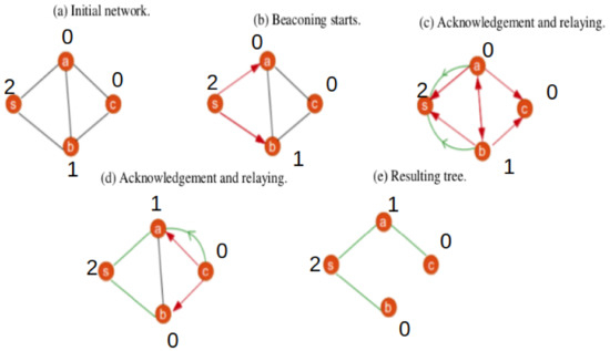
Figure 1.
Routing with LIBA.
Figure 1 illustrates the basic steps of a typical collection tree protocols which is LIBA. We assume a certain number of routing rounds and hence assume an initially node-weighted graph. Figure 1a shows the structure of the considered current subnetwork. It reveals that the considered node weighting is described as in the dictionary = {s:2, a:0, b:1, c:0}. It is shown in Figure 1b that the sink s (this is the uniquely assumed sink) starts the beaconing process by broadcasting a beaconing message. As shown in Figure 1c, each node receiving the beaconing message (initiated from the sink) chooses the parent (sender) and relays the beacon in the network.The figure also shows that the acknowledged node updates its weight to the number of the acknowledgment messages received. This is why the sink’ s weight remains at 2. Figure 1d shows that node c chooses and acknowledges node a because it has the least weight (level of interference). This updates the weight of node a, whereas nodes b and c update their weights to zero, as they have not received any acknowledgment message. This means that there are no parents to any node in the resulting routing tree. The new weighting distribution then becomes = {s:2, a:1, b:0, c:0}, and the overall weight distribution is therefore = {s:4, a:1, b:1, c:0}.
This scheme is periodically repeated for nodes to make new choices and hence update their paths leading to the sink.
For as long as the algorithm keeps on being repeated, nodes increase their weights (levels of interference). Here, it is important to note that the increase in interference of one node does not affect the increase in interference for each node of the network. Rather, it causes the increase in interference of a selected group of nodes. For instance, it is clear from Figure 1 that the high level of interference of node b would influence the interference choice of node c, which would prefer node a of a lower weight and, consequently, node a would increase its weight. If the weight of node a becomes higher than that of b, for the same reason, node b would increase its weight. This means that the increase in weight/interference on node b affects the increase in weight on node a and vice versa, and no other node in the network is affected by the level of interference of any of the two nodes.
Hence, the interference spread is group dependent. We call these group of nodes diffusion sets. In the next section, we study the diffusion sets structure, and this will enable us to study the interference spread across the underlying network.
3. Diffusion Set I
Having seen that the spread of interference depends on some subsets structure of the network, we mathematically study a new structure of nodes in a network, based on how nodes can spread interference to each other. We refer to the fact that an increase in interference level (weight) of a node may cause other selected nodes to increase their weights, and in this case we say that interference is transferred from one node to another.
So, modeling the interference spread in a WSN which uses collection tree algorithms, such as LIBA, depends on the interference spread within each diffusion set of the network. The spread of interference does not behave in the same way for all diffusion sets, and this is why the global spread modeling has to depend on modeling the spread on each diffusion set of the network.
However, the quantification of nodes would be difficult in the case where a node can belong in more than one diffusion sets. This is why, in this section, we study the structure of the diffusion sets and their properties leading to the network partition, before conducting any quantitative modeling. The claimed partition property will give us confidence that, once the quantitative modeling is done on the level of the diffusion set, no node in the network is counted more than once.
We start by formally defining the diffusion set and prove all lemmas and theorems leading to the partition property. Here, we depend on the definition of a partition stating that a set of subsets is a partition of a set S if, and only if, all subsets in are mutually exclusive and their union equals S. We aim to prove that the set of diffusion sets is a partition of the set of nodes of the underlying network.
Definition 1.
Consider to be an undirected and node-weighted network where L stands for the set of its links, N is the set of its nodes, W is the set of the nodes weights and s is its sink. Define on N a distance function such that is the least number of links between node n and the sink s of the graph G.
A diffusion set I is a non empty subset of N satisfying the following properties:
- P1:All nodes in set I are at the same distance from the sink. That is,
- P2:I is a singleton, or for each node x in I, there is another node y in I such that x and y share the next neighbor (the next node, say, z of the node n refers to a node such that and . Mathematically,
- P3:For each node x in N, if x shares a next node with some node in I, then . That is,
To define the diffusion set, we adopted the general definition provided in [38] by using a special distance function.
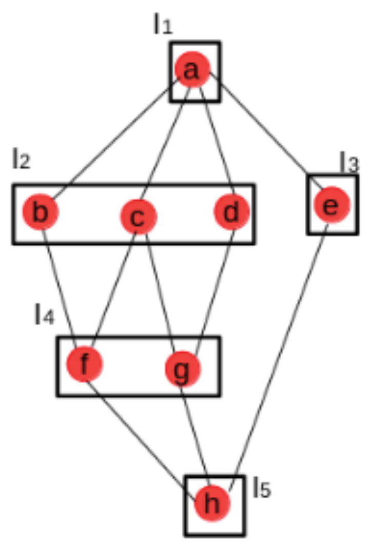
Figure 2 represents an example which shows the graph whose nodes are partitioned in diffusion sets.

Figure 2.
Diffusion sets.
From Figure 2, nodes are grouped in diffusion sets as follows:
- ,
- ,
- ,
- and
- .
It is clear that the union of all diffusion sets consists of all nodes of the graph, and all diffusion sets of the graph are mutually exclusive.
Thus, the set {} of all diffusion sets forms a partition of the set N. The figure also shows that any two nodes in the same diffusion set do not need to have the same next neighbor. For instance, nodes b and d are in the same diffusion set but do not have the same next neighbor: the next neighbor of b is f, whereas the next neighbor of d is g.
Furthermore, the nodes e and g (or f) share the same next neighbor h, but they are not in the same diffusion set because they are not at the same distance from the sink a. In fact, but and clearly .
Lemma 1.
Consider the set of all diffusion sets of a graph (see Definition 1). Each diffusion set I of G is maximal in . That is,
Proof.
Let and be two diffusion sets such that .
We want to show that . Since , it is sufficient to show that because .
We proceed by contradiction.
Let . This means that and x∉. Since , property in Definition 1 is valid. That is,
Taking the contrapositive and using the fact that x∉,
On the other hand implies that
So, there is no node which shares the next node with the node x. It follows that no node in can be in the same diffusion set as x. This contradicts the fact that nodes in and x are in the same diffusion set . □
In two steps (Theorems 1 and 2), we prove that the set of diffusion sets partitions the set of all nodes of the network .
Theorem 1.
Given the graph as described in Definition 1, the set of all diffusion sets of G are pairwise disjoint. That is,
Proof.
Let and be any two diffusion sets. We want to show that
Let .
If both and are singletons, then we are done.
If is a singleton and is not, implies that and hence because and are maximal in ( Lemma 1).
Consider and to be two diffusion sets of size greater than 1, and let us proceed by contradiction.
Let and suppose ( and if not which contradicts Lemma 1). It follows that there is no node belonging to , sharing its next neighbor with the node y.
Since , there is no node in sharing the next hop with the node y.
Hence, by property in Definition 1 (definition of diffusion set), there is no node in belonging in the same diffusion set as the node y.
This implies that the nodes x and y are not in the same diffusion set.
On the other hand, implies that , and implies that ; this contradicts the fact that the nodes x and y do not belong in the same diffusion set. Hence . □
Theorem 2.
Let be the set of all diffusion sets of the graph (see Definition 1). For each node x in N, there exists a diffusion set I in containing x. That is,
Proof.
For , we want to find a diffusion set which contains x. Define a subset M of N satisfying the following characteristics:
- :
- All nodes in M are at the distance . That is,
- :
- , or for each node n in M there is another node y in M such that n and y share a next neighbor. That is,
- :
- For each node n in N, if n shares a next neighbor with node y in M, then n is a member of M. That is,
- :
- x shares a next neighbor with a node y in M. That is,
Since and is valid, shows that (by setting ).
On the other hand , and (see Definition 1), and hence . Thus
□
Corollary 1.
The set of all diffusion sets of the network (see Definition 1) partitions N.
Proof.
By definition in Definition 1, consists of nonempty elements. In addition, Theorem 1 shows that consists of disjoints elements. It is then sufficient to show that the union of the sets in is equal to N. That is
since , and thus, by Definition 1, , . Hence,
On the other hand, from Theorem 2 it follows that
Note that since is a partition of the set N of all nodes of a network, we can say that
This helps us make a quantitative study involving diffusion sets.
4. Interference Spread Model
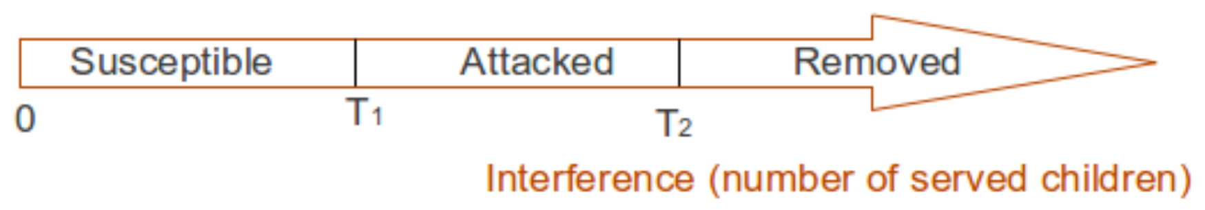
Based on usual mechanisms of epidemic disease spread, we propose a model for interference spread in a network when LIBA is the typically used collection tree protocol. In this work, the nodes are considered to be distributed in three epidemic compartments and we need two thresholds and to specify susceptible, attacked or replaced nodes, as shown by Figure 3.

Figure 3.
Thresholds for interference states subdivision.
Figure 3 enables us to define the considered states as follows:
- Susceptible nodes: They are the nodes that interfere less or do not interfere in a network, and their total number is denoted by S. Each susceptible node is assumed to have a weight less than the threshold .
- Attacked nodes: They are the highly interfering nodes, but still are able to operate. The total number of attacked nodes in a network is denoted by A. An attacked node is assumed to have a weight less than the threshold but at least to the threshold .
- Replaced nodes: They are the nodes which are replaced because of the high interference. These nodes’ total number is denoted by R. A node is considered to be replaced if its interference is at least the threshold .
To show the interference spread mechanisms, We use Figure 4 to picture the cases considered, and this enables us to clarify the underlying model assumptions.
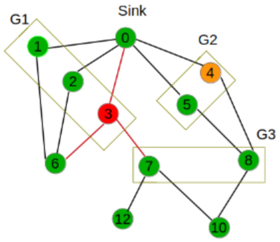
Figure 4.
Interference transmission in the diffusion sets of a network.
As depicted from Figure 4, the assumed network is partitioned in diffusion sets G1, G2, G3 and singletons. Node 4 is attacked, and this attack can only affect Node 4. Node 3 is viewed as a node which has been replaced due to a very high level of interference. Nodes in the same diffusion set as Nodes 3 and 4, together with the remaining nodes in the network, are assumed to be susceptible.
We assume that replaced nodes do not become infected or susceptible again. The reason is that nodes might be replaced with high quality and they would be attacked once the majority of the original nodes in the network have been replaced. In this case, all replaced nodes are updated to susceptible, and other compartments are assumed to be empty; then the dynamic model is applied again.
4.1. The Proposed Spread Model
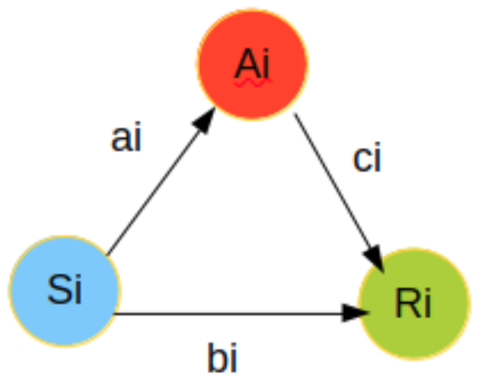
Nodes may be distributed in diffusion sets (see the algorithm in [38]), where nodes in the same diffusion set are assumed to be infectiously similar to each other and those in different diffusion sets behave differently. Each diffusion set i contains a set of susceptible nodes whose number is denoted by , the set of attacked nodes whose size is and finally the set of replaced nodes whose size is . A diffusion set i in which or is referred to as the attacked set, that is, the diffusion set which has contained at least one attached or replaced node. The following figure shows the considered compartmental migration rates in any arbitrary diffusion set, say, i.
As shown in Figure 5, Susceptible nodes in the diffusion set i may be attacked at the rate , whereas attacked nodes from i are replaced at the rate .

Figure 5.
Representation of interference spread.
Susceptible nodes in the diffusion set i may quickly increase their interference levels so as to be directly replaced without being considered as attacked. On the other hand, replaced nodes my cause some of the susceptible or attacked nodes to leave the network because of the destruction of links. We consider to be the rate with which susceptible nodes in i are replaced.
4.2. Analytical Description
Taking account to all cases discussed in Section 4.1, we obtain the following difference equation.
Note that , and are functions of time t for each diffusion set i. The negative rates in the model represent a decrease, whereas the positive ones represent an increase.
The parameter stands for the transmission rate between susceptible and attacked nodes. This parameter depends directly on the number of susceptible nodes and the attacked ones . This is why it makes sense to say that relates two other measures:
- The susceptibility rate of each node in the interference group i which is denoted by .
- Infectiousness rate of nodes in the attacked diffusion set i denoted by .
On the other hand, the structure of a diffusion set clearly influences the attack ability since different diffusion sets have not the same infection effects. We use the parameter for the measure of the structure impact when a node is attacked.
So to compute , we use the formula
where denotes the fraction of attacked nodes in diffusion set i.
4.3. Model Assumptions
- We assume that there is no node newly joining the network. That is, at any time t, if N is the number of nodes at time , then .
- The death (not caused by interference) and birth rate are assumed to be zero.
- We consider the networks where the death of nodes does not cause new diffusion set formation.
4.4. Stability Analysis
In this section, we study the stability of the system at the disease-free equilibrium points. We first compute the disease-free equilibrium of the system which is used to computer the basic reproduction number , which is the number used for studying the stability.
4.5. Disease-Free Equilibrium (DFE)
Consider Equation (5) and assume the sets of the network diffusion sets in whose size is m. Since the system is not affected by the number of replaced nodes R, the equation of R is omitted. We present DFE as , which verifies the equations
Since , Equation (6) is reduced to
- Case 1:
- If , then , is the unique solution of Equation (8). In this case, the DFE is .
- Case 2:
- If , then the system of Equation (8) has infinitely many solutions, and thus the system will have infinite number of DFE whose form is where may not all be zero.
Note that according to linear algebra, if, and only if, the rows or columns of A are linearly dependent. This can help us to study the dependency of diffusion sets in terms of interference transmission.
4.6. Stability of a Network at DFE
We study stability using the basic reproduction number . We calculate using the next-generation matrix approach as described in [39].
After removing the equations for , let us decompose the remaining systems of Equation (7) into two subsystems as follows:
The next-generation matrix is , where F and V are the Jacobian matrices of and , respectively, evaluated at the DFE.
- Case 1:
- If , the DFE is , and the Jacobian of evaluated at is , the zero matrix.Consequently, the matrix is the zero matrix. The eigenvalues of the matrix K are all zero and hence the basic reproductive number is . Since , the DFE is globally stable. This is explained by the fact that at , the network is empty and will remain empty because no new nodes join it.
- Case 2:
- If , then the system of Equation (8) has more than one solutions, and thus the system will have more than one DFE points whose form is , where may not all be zero.
Since K is a diagonal matrix, the basic reproduction number is
5. Numerical Results
In this section, numerical results are computed using three different settings.
- Static system. It is a system where parameters are considered constants.
- Stochastic system. It is the system where parameters are randomly selected.
- Predictive system. It is a system where parameters are assumed to follow a predictive function.
We use the subnetworks in Figure 6 to explain the network scenarios where the three systems may be applicable. A focus is put on the diffusion sets , and as shown in Figure 6a–c, respectively. We assume all nodes in the same diffusion set have exactly the same initial weights. This assumption is possible in many ways: for instance, at the first run of the LIBA, where nodes have not yet chosen their parent and their weights are all zero.
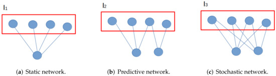
Figure 6.
Considered types of networks.
As it is shown in Figure 6a, all nodes in diffusion set are connected to only one next node, which has to choose any of the nodes in as the parent. The nodes in the diffusion set have the same weights and hence they have an equal chance to be chosen to be parent. So for each run of LIBA, exactly one node of the diffusion set is increased by one. Furthermore, an already chosen node increases the weight and will have a chance to be chosen again, once each node has been chosen and has incremented its weight by 1 to obtain the same weights for all nodes in the diffusion set. So, given the number of runs, one can compute the number of nodes which have achieved a certain level of interference. The average of such a number of nodes will determine how many nodes are expected to achieve a certain interference threshold and, hence, how many nodes would change a compartment. However, Figure 6b shows a case where nodes do not have the same chance to be chosen as the parent. There is clearly a node in the diffusion set which may be chosen by two next nodes. This makes it difficult to calculate how many nodes will have achieved a certain level of interference, given the number of runs. We say that such a number is random. However, the scenario presented in Figure 6c shows a more randomized scenario, where it is harder to make such a prediction. In this case, we assume that the rates of the compartment transmission are random (stochastic) in the case of the network in Figure 6c, but in the case of Figure 6b, the randomness appears biased. This is why, in the case of Figure 6b, more investigations have to be conducted by recording various rates, using some predictive techniques to approximate such rates.
5.1. Static System
Table 2 shows the initial conditions of the considered network and also the constant values of the considered parameters. It enabled us to use the Euler method (see [40]) to numerically solve Equation (3). Python packages were used in simulation (numerical computation and plotting of related curves) where the solution was computed with 5999 iterations.
Table 2.
Numerical values.
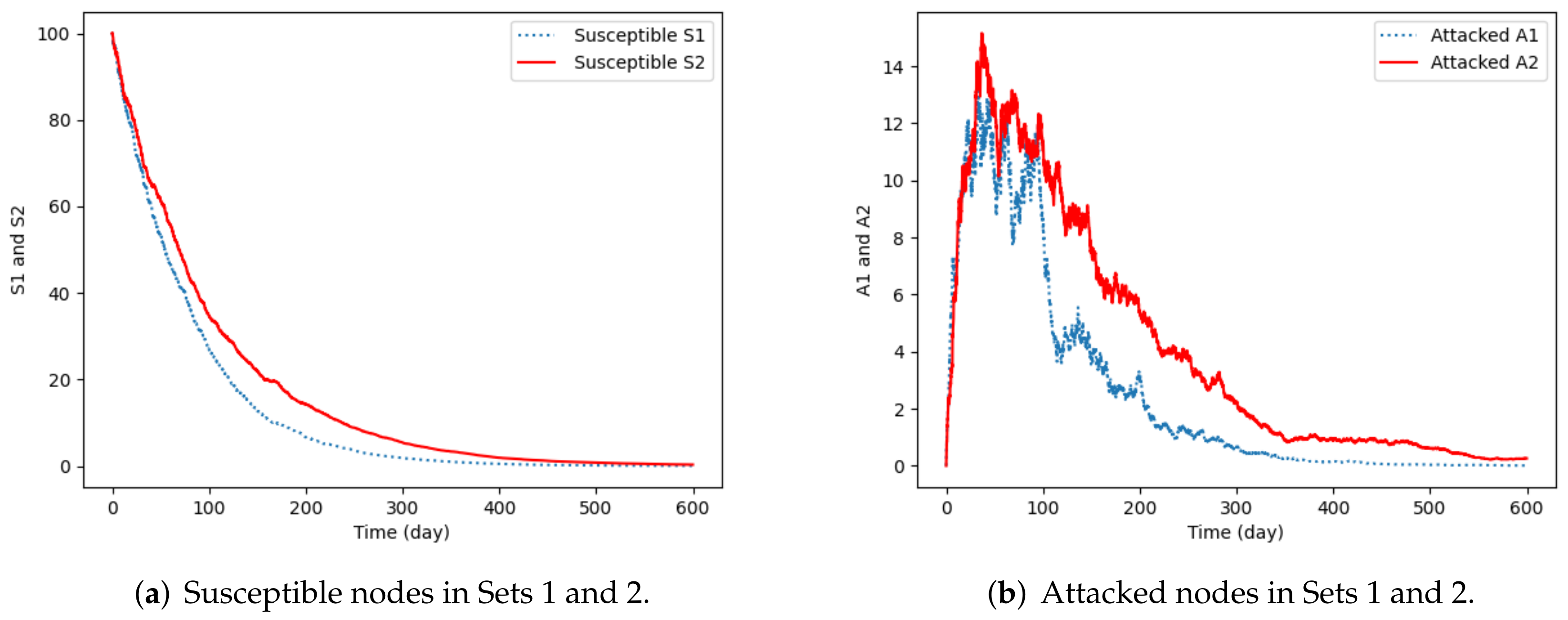
Figure 7 represents the trend of compartment sizes when related parameter/rates are assumed to be constant. Figure 7a shows that the number of susceptible nodes, in both diffusion sets, decreases quickly toward their convergence to zero, after 500 days.
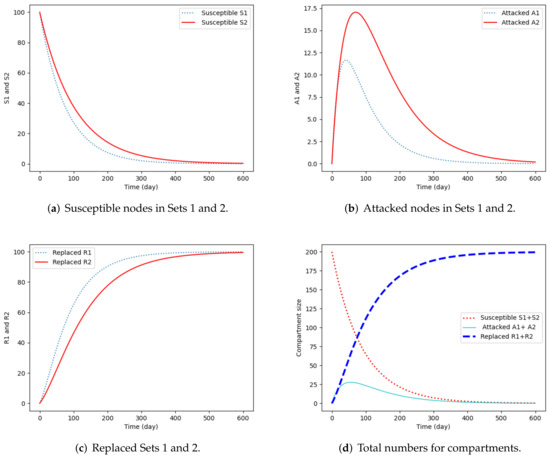
Figure 7.
Interference spread in a static system.
Figure 7b shows that attacked nodes for both diffusion sets first increase toward a single maximum, then decrease toward the convergence to zero after 600 days.
Figure 7c reveals that the number of replaced nodes increases and converges at the total number of nodes in each diffusion set (100 nodes), and this is highlighted in Figure 7d.
It is important to note that the difference in variation rates reflects the parameter settings shown in Table 2. This also justifies the reason why the number of attacked nodes do not reach the same maximum.
5.2. Stochastic System
We consider a system where the parameters are randomly selected. The selection is done in a normally distributed sample (with sample size 5999) of values shown in Table 3. We use the representation, such as , to mean that the parameter for the first set is selected from a normal distribution whose mean is and the standard deviation is .
Table 3.
Numerical values.
Figure 8 shows the same trend as Figure 7, except the fact that the curves in Figure 8 are not smooth, and this causes the system not to have unique maximum of attacked nodes (for each diffusion set), unlike the case of static system (Figure 7).
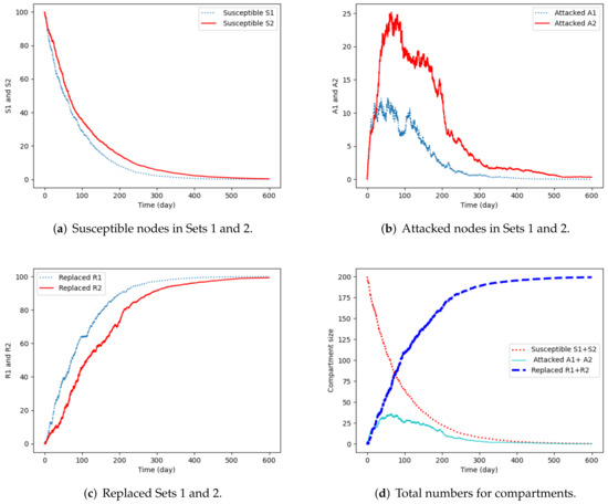
Figure 8.
The interference spread stochastic system.
5.3. Predictive System
In this experiment, parameters are considered to be functions of time. We assume that they may be predicted by a Gaussian function. The considered distribution for each parameter is the same as in a stochastic system. However, in this experiment, instead of randomly selecting values of parameters, the order in which the sample values are distributed is respected.
Figure 9 shows that the predictive system differs from the stochastic system, only with respect to the fact that curves corresponding to diffusion set may cross each other.
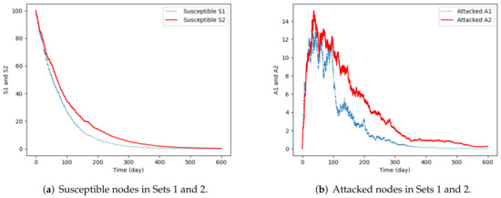
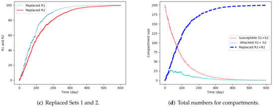
Figure 9.
The interference spread in a predictive system.
6. Conclusions
In this paper, the diffusion set is a new structure of nodes in a network. The properties of diffusion sets leading to the partition property was proven and hence justified the model on the diffusion set model. This enabled quantitative modeling of the interference spread on the network. We presented a SAR model describing the spread of interference when LIBA is used by the network. Results showed that for static, stochastic and predictive systems, susceptible nodes and attacked nodes converge to zero, whereas the replaced nodes converge to the total number of nodes in each diffusion set. All used data are artificial. For future work, it is essential to use real data, where the static system is determined using approximated parameters and the predictive system is defined using predictive models obtained by regression analysis.
Author Contributions
Conceptualization, E.T.; methodology, E.T.; software, E.T.; validation, J.d.D.N., F.M.T., J.U.R., P.G., A.B. and E.N.; formal analysis, E.T.; investigation, E.T.; resources, E.T. and A.B.; data curation, J.d.D.N., F.M.T., J.U.R., P.G. and E.N.; writing—original draft preparation, E.T.; writing—review and editing, E.T., J.d.D.N., F.M.T., J.U.R., P.G., A.B. and E.N.; visualization, E.T., J.d.D.N., F.M.T., J.U.R., P.G. and E.N.; supervision, A.B.; project administration, E.T. and A.B. All authors have read and agreed to the published version of the manuscript.
Funding
This research received no external funding.
Informed Consent Statement
Not applicable.
Data Availability Statement
Not applicable.
Conflicts of Interest
The authors declare no conflict of interest.
Acronyms
| IoT | internet of things |
| LIBA | least interference beaconing algorithm |
| SAR | susceptible–attacked–replaced |
| WSN | wireless sensor network |
| SIS | susceptible–infected–susceptible |
| SIP | susceptible–infected–protected |
| SIRS | susceptible–infected–recovered (removed) susceptible |
| SIR | susceptible–infected–recovered |
| SIR-M | susceptible–infected–recovered with maintenance |
| CTP | collection tree protocol |
| IP | internet protocol |
| IR | infected and recovered |
| TOB | TinyOS beaconing |
| 4IR | fourth industrial revolution |
References
- Schwab, K. The Fourth Industrial Revolution; Currency: Redfern, NSW, Australia, 2017. [Google Scholar]
- Shah, S.H.; Yaqoob, I. A survey: Internet of Things (IOT) technologies, applications and challenges. In Proceedings of the 2016 IEEE Smart Energy Grid Engineering (SEGE), Oshawa, ON, Canada, 21–24 August 2016; pp. 381–385. [Google Scholar]
- Kortuem, G.; Kawsar, F.; Sundramoorthy, V.; Fitton, D. Smart objects as building blocks for the internet of things. IEEE Internet Comput. 2009, 14, 44–51. [Google Scholar] [CrossRef] [Green Version]
- Mauwa, H.; Bagula, A.; Tuyishimire, E.; Ngqondi, T. An optimal spectrum allocation strategy for dynamic spectrum markets. In Proceedings of the 2019 International Conference on Wireless and Mobile Computing, Networking and Communications (WiMob), Barcelona, Spain, 21–23 October 2019; pp. 1–8. [Google Scholar]
- Mauwa, H.; Bagula, A.; Tuyishimire, E.; Ngqondi, T. Community healthcare mesh network engineering in white space frequencies. In Proceedings of the 2019 ITU Kaleidoscope: ICT for Health: Networks, Standards and Innovation (ITU K), Atlanta, GA, USA, 4–6 December 2019; pp. 1–8. [Google Scholar]
- Tuyishimire, E.; Adiel, I.; Rekhis, S.; Bagula, B.A.; Boudriga, N. Internet of Things in Motion: A Cooperative Data Muling Model under Revisit Constraints. In Proceedings of the Ubiquitous Intelligence & Computing, Advanced and Trusted Computing, Scalable Computing and Communications, Cloud and Big Data Computing, Internet of People, and Smart World Congress (UIC/ATC/ScalCom/CBDCom/IoP/SmartWorld), 2016 International IEEE Conferences, Toulouse, France, 18–21 July 2016; pp. 1123–1130. [Google Scholar]
- Antoine, B.; Tuyishimire, E.; Olasupo, A. Cyber physical systems (cps) surveillance using an epidemic model. arXiv 2019, arXiv:1912.07479. [Google Scholar]
- Darvishi, H.; Ciuonzo, D.; Eide, E.R.; Rossi, P.S. Sensor-fault detection, isolation and accommodation for digital twins via modular data-driven architecture. IEEE Sens. J. 2020, 21, 4827–4838. [Google Scholar] [CrossRef]
- Santamaria, A.F.; Raimondo, P.; Tropea, M.; De Rango, F.; Aiello, C. An IoT surveillance system based on a decentralised architecture. Sensors 2019, 19, 1469. [Google Scholar] [CrossRef] [PubMed] [Green Version]
- Ismail, A.; Bagula, B.A.; Tuyishimire, E. Internet-of-things in motion: A uav coalition model for remote sensing in smart cities. Sensors 2018, 18, 2184. [Google Scholar] [CrossRef] [PubMed] [Green Version]
- Ismail, A.; Tuyishimire, E.; Bagula, A. Generating dubins path for fixed wing uavs in search missions. In International Symposium on Ubiquitous Networking; Springer: Berlin/Heidelberg, Germany, 2018; pp. 347–358. [Google Scholar]
- Tuyishimire, E. Cooperative Data Muling Using a Team of Unmanned Aerial Vehicles. Ph.D. Thesis, University of the Western Cape, Cape Town, South Africa, 31 July 2019. [Google Scholar]
- Tuyishimire, E.; Bagula, A.; Rekhis, S.; Boudriga, N. Trajectory Planing for Cooperating Unmanned Aerial Vehicles in the IoT. IoT 2022, 3, 147–168. [Google Scholar] [CrossRef]
- Bagula, A.; Tuyishimire, E.; Wadepoel, J.; Boudriga, N.; Rekhis, S. Internet-of-Things in Motion: A Cooperative Data Muling Model for Public Safety. In Proceedings of the Ubiquitous Intelligence & Computing, Advanced and Trusted Computing, Scalable Computing and Communications, Cloud and Big Data Computing, Internet of People, and Smart World Congress (UIC/ATC/ScalCom/CBDCom/IoP/SmartWorld), 2016 International IEEE Conferences, Toulouse, France, 18–21 July 2016; pp. 17–24. [Google Scholar]
- Tuyishimire, E.; Bagula, A.; Rekhis, S.; Boudriga, N. Cooperative Data Muling from Ground Sensors to Base Stations Using UAVs. In Proceedings of the 2017 IEEE Symposium on Computers and Communications (ISCC), Heraklion, Greece, 3–6 July 2017. [Google Scholar]
- Snoonian, D. Smart buildings. IEEE Spectr. 2003, 40, 18–23. [Google Scholar] [CrossRef]
- Lund, H.; Østergaard, P.A.; Connolly, D.; Mathiesen, B.V. Smart energy and smart energy systems. Energy 2017, 137, 556–565. [Google Scholar] [CrossRef]
- Haverkort, B.R.; Zimmermann, A. Smart industry: How ICT will change the game! IEEE Internet Comput. 2017, 21, 8–10. [Google Scholar] [CrossRef]
- Baig, M.M.; Gholamhosseini, H. Smart health monitoring systems: An overview of design and modeling. J. Med. Syst. 2013, 37, 1–14. [Google Scholar] [CrossRef]
- Tuyishimire, E.; Bagula, B.A.; Ismail, A. Optimal clustering for efficient data muling in the internet-of-things in motion. In International Symposium on Ubiquitous Networking; Springer: Berlin/Heidelberg, Germany, 2018; pp. 359–371. [Google Scholar]
- Tuyishimire, E.; Bagula, A.; Ismail, A. Clustered data muling in the internet of things in motion. Sensors 2019, 19, 484. [Google Scholar] [CrossRef] [PubMed] [Green Version]
- Jibreel, F.; Tuyishimire, E.; Daabo, I.M. An Enhanced Heterogeneous Gateway-Based Energy-Aware Multi-hop Routing Protocol for Wireless Sensor Networks. Preprints 2022, 2022010024. [Google Scholar] [CrossRef]
- Tuyishimire, E. Routing in Mobile Networks. 2013. Available online: https://tinyurl.com/5n7ppvh5 (accessed on 10 February 2022).
- Tuyishimire, E.; Bagula, B.A. A Formal and Efficient Routing Model for Persistent Traffics in the Internet of Things. In Proceedings of the 2020 Conference on Information Communications Technology and Society (ICTAS), Durban, South Africa, 11–12 March 2020; pp. 1–6. [Google Scholar]
- Bagula, A.B.; Djenouri, D.; Karbab, E. On the Relevance of Using Interference and Service Differentiation Routing in the Internet-of-Things. In Internet of Things, Smart Spaces, and Next Generation Networking; Springer: Berlin/Heidelberg, Germany, 2013; pp. 25–35. [Google Scholar]
- Bagula, A.; Djenouri, D.; Karbab, E. Ubiquitous Sensor Network Management: The Least Interference Beaconing Model. In Proceedings of the 2013 IEEE 24th Annual International Symposium on Personal, Indoor, and Mobile Radio Communications (PIMRC), London, UK, 8–11 September 2013. [Google Scholar]
- Ngqakaza, L.; Bagula, A. Least Path Interference Beaconing Protocol (LIBP): A Frugal Routing Protocol for the Internet-of-Things. In International Conference on Wired/Wireless Internet Communications; Springer: Berlin/Heidelberg, Germany, 2014; pp. 148–161. [Google Scholar]
- Azmi, N.; Kamarudin, L.; Mahmuddin, M.; Zakaria, A.; Shakaff, A.; Khatun, S.; Kamarudin, K.; Morshed, M. Interference issues and mitigation method in WSN 2.4 GHz ISM band: A survey. In Proceedings of the 2014 2nd International Conference on Electronic Design (ICED), Penang, Malaysia, 19–21 August 2014; pp. 403–408. [Google Scholar]
- Denis Ndanguza, J.; de Dieu Niyigena, J.M.T. Modelling the Distribution and Spread of Ebola Disease in West Africa; Nova Science Publishers: Hauppauge, NY, USA, 2019; Chapter 1. [Google Scholar]
- Kermack, W.; McKendrick, A. Contributions to the mathematical theory of epidemics—I. Bull. Math. Biol. 1991, 53, 33–55. [Google Scholar] [PubMed]
- Theodorakopoulos, G.; Le Boudec, J.Y.; Baras, J.S. Selfish response to epidemic propagation. IEEE Trans. Autom. Control 2012, 58, 363–376. [Google Scholar] [CrossRef] [Green Version]
- Ganesh, A.; Massoulié, L.; Towsley, D. The effect of network topology on the spread of epidemics. In Proceedings of the IEEE 24th Annual Joint Conference of the IEEE Computer and Communications Societies, Miami, FL, USA, 13–17 March 2005; Volume 2, pp. 1455–1466. [Google Scholar]
- Sotoodeh, H.; Safaei, F.; Sanei, A.; Daei, E. A General Stochastic Information Diffusion Model in Social Networks based on Epidemic Diseases. arXiv 2013, arXiv:1309.7289. [Google Scholar] [CrossRef]
- Zhang, X.; Neglia, G.; Kurose, J.; Towsley, D. Performance modeling of epidemic routing. Comput. Netw. 2007, 51, 2867–2891. [Google Scholar] [CrossRef]
- Tang, S.; Mark, B.L. Analysis of virus spread in wireless sensor networks: An epidemic model. In Proceedings of the 2009 7th International Workshop on Design of Reliable Communication Networks, Washington, DC, USA, 25–28 October 2009; pp. 86–91. [Google Scholar]
- Tuyishimire, E.; Bagula, B.A. Modelling and analysis of interference diffusion in the internet of things: An epidemic model. In Proceedings of the 2020 Conference on Information Communications Technology and Society (ICTAS), Durban, South Africa, 11–12 March 2020; pp. 1–6. [Google Scholar]
- Wei, Z.; Masouros, C.; Liu, F.; Chatzinotas, S.; Ottersten, B. Energy-and cost-efficient physical layer security in the era of IoT: The role of interference. IEEE Commun. Mag. 2020, 58, 81–87. [Google Scholar] [CrossRef]
- Tuyishimire, E.; Bagula, B.A. A novel management model for dynamic sensor networks using diffusion sets. In Proceedings of the 2020 Conference on Information Communications Technology and Society (ICTAS), Durban, South Africa, 11–12 March 2020; pp. 1–6. [Google Scholar]
- Roberts, M.G.; Heesterbeek, J. Characterizing the next-generation matrix and basic reproduction number in ecological epidemiology. J. Math. Biol. 2013, 66, 1045–1064. [Google Scholar] [CrossRef] [PubMed] [Green Version]
- Hahn, G. A modified Euler method for dynamic analyses. Int. J. Numer. Methods Eng. 1991, 32, 943–955. [Google Scholar] [CrossRef]


Publisher’s Note: MDPI stays neutral with regard to jurisdictional claims in published maps and institutional affiliations. |
© 2022 by the authors. Licensee MDPI, Basel, Switzerland. This article is an open access article distributed under the terms and conditions of the Creative Commons Attribution (CC BY) license (https://creativecommons.org/licenses/by/4.0/).