Audio Classification Algorithm for Hearing Aids Based on Robust Band Entropy Information

Abstract

Audio classification algorithms for hearing aids require excellent classification accuracy. To achieve effective performance, we first present a novel supervised method, involving a spectral entropy-based magnitude feature with a random forest classifier (SEM-RF). A novel-feature SEM based on the similarity and stability of band signals is introduced to improve the classification accuracy of each audio environment. The random forest (RF) model is applied to perform the classification process. Subsequently, to resolve the problem of decreasing classification accuracy of the SEM-RF algorithm in mixed speech environments, an improved algorithm, ImSEM-RF, is proposed. The SEM features and corresponding phase features are fused on multiple time resolutions to form a robust multi-time resolution magnitude and phase (multi-MP) feature, which improves the stability of the feature with which the speech signal interferes. The RF model is improved using the linear discriminant analysis (LDA) method to form a linear discriminant analysis-random forest (LDA-RF) joint classification model, which performs model acceleration. Through experiments on hearing aid research data sets for acoustic environment recognition, the effectiveness of the SEM-RF algorithm was confirmed on a background audio signal dataset. The classification accuracy increased by approximately 7% compared with the background noise classification algorithm using an RF tree classifier. The validity of the ImSEM-RF algorithm in speech-interference environments was confirmed using the speech in the background audio signal dataset. Compared with the SEM-RF algorithm, the classification accuracy was improved by approximately 2%. The LDA-RF reduced the program’s running time by >80% with multi-MP features compared with RF.

1. Introduction

A digital hearing aid system should recognize the use environment, such as quiet indoor areas, concerts, and noisy traffic environments. Consequently, the signal processing algorithms and parameters can be adjusted according to the current environment. Classification algorithms generally generate control signals for processing chains. High-performance digital hearing aids require a classification algorithm to achieve audio classification capability. Therefore, an appropriate audio signal processing algorithm and parameter configuration can be adjusted according to the surrounding environment to improve product performance and user experience [1,2,3,4,5].

The audio scene classification algorithm mainly concentrates on feature extraction and model selection. Sub-band periodicity, sub-band entropy, and sub-band energy ratio are the typical band classification features applied for audio classification. Rule-based classification, minimum distance-based classification, and statistical model-based classification methods such as threshold methods, k-nearest neighbor (KNN), support vector machine (SVM), Gaussian mixed models (GMM), hidden Markov models (HMM), and artificial neural networks (ANNs), have been adopted for audio classification problem [6,7,8]. For hearing auxiliary equipment, such as hearing aids and cochlear applications classification algorithms have been improved and optimized according to their excellent accuracy. Nordqvist et al. [9] proposed an efficient and robust hearing aid classification algorithm based on HMM. The algorithm can automatically adjust usage patterns in the environment according to personal preferences. Büchler et al. [10] designed audio classification systems for hearing aids using feature extraction with auditory scene analysis. Lamarche et al. [11] proposed the use of an adaptive audio classification framework. It has been proven that an adaptive system can split or merge classes according to the current environment using minimum distance clustering and a Bayesian classifier. Random forest (RF) was first applied to cochlea background noise classification in 2014. Combined with band features, the algorithm achieves high classification accuracy and real-time implementation [12]. The real-time implementation of this algorithm was conducted on both Android and iOS smartphones [13]. The average processing times per 25 ms frames with a frame overlap of 12.5 ms for the sub-band+RF classification on the Android platform (Nexus 5) and IOS platform (iPad Mini 2) were <4 ms. Alavi et al. [14] proposed a noise classification algorithm for cochlear applications. Mel-scale frequency cepstral coefficient (MFCC) features, GMMs and Bayesian classifiers were adopted to provide automation solutions for noise reduction in different environments. Existing algorithms based on RF and band features are mainly focused on the classification of background noise, but communication during the use of hearing aids is a universal topic. The speech signal received in communication affects the stability of the classification features of the current environment audio signal. Voice activity detection (VAD) [15,16] is usually adopted to detect background noise paragraphs and background noise paragraph-containing speech signals. Thereafter, the classification algorithm is applied to the noise section to reduce the classification error rate and maintain the algorithm’s classification accuracy. In 2020, the Center of Competence for Hearing Systems in Germany proposed a novel, binaural hearing aid acoustic environment recognition dataset (HEAR-DS) [17] that is suitable for the environment recognition needs of hearing aids. Various deep neural network-based classifiers with varying complexity were trained to show the separability of these acoustic environments. They implemented a live evaluation system in C++ on an Intel i7 7th gen NUK. The most complex network they used took less than 0.4 s for every 10 s of live audio. The acoustic environments in this dataset were categorized into three groups. The speech group consisted inherently of speech. The acoustic environments in the background group contained pure background noise, and the speech in the background group consisted of acoustic environments with a target speaker embedded in one of the backgrounds.

To meet the challenge of the effective classification of hearing aids, a novel supervised method, a spectral entropy-based magnitude feature with a random forest classifier (SEM-RF), is presented in this study. To solve the problem of decreasing the classification accuracy of the SEM-RF algorithm in mixed speech environments, an improved algorithm ImSEM-RF is presented. The main contributions of this study are as follows:

• To achieve effective performance, we first present a novel supervised method, SEM-RF. A novel-feature SEM based on the similarity and stability of band signals is introduced to improve the classification accuracy of each audio environment. An RF model was applied to perform high-speed classification.
• For the problem of the decreasing classification accuracy of the SEM-RF algorithm in speech mixed environments, ImSEM-RF is proposed. The SEM features and corresponding phase features are fused on multiple time resolutions to form a multi-MP feature, which improves the stability of the feature with which the speech signal interferes.
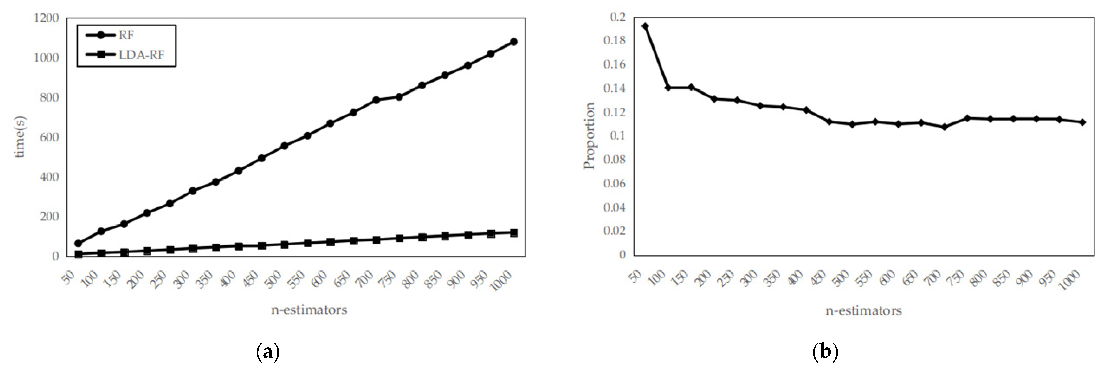
• An improved ensemble learning method based on linear discriminant analysis and random forest, LDA-RF, is proposed. High-dimensional features are converted into low-dimensional features to reduce redundant information and time complexity. The calculation speed is accelerated during model training and prediction.

The remainder of this paper is organized as follows. In Section 2, the details of SEM-RF are described. Section 3 introduces the proposed robust multi-time resolution fusion feature based on the magnitude-phase feature. Section 4 presents the ImSEM-RF algorithm. Section 5 presents the experimental results. The conclusions are presented in Section 6.

2. SEM-RF Method

The details of the SEM-RF algorithm, including the feature extraction and classification model, are as follows.

2.1. Band Spectral Feature

The classification features of hearing aids should obtain the natural characteristics of audio signals effectively. A single feature often reflects the characteristics of certain aspects of the signal. However, audio signals in different environments are typically composed of signals generated by multiple sources, such as car noise, including wind, tire, and engine noise. Therefore, jointed features can comprehensively describe the characteristics of audio signals by combining features in different aspects. Band features can effectively classify different types of audio signal because of their detailed descriptions in each frequency domain. Band spectrum entropy features are widely used in VAD to separate speech signals from background noise [18]. This is an effective feature of signal classification. However, the band spectral entropy only indicates the signal characteristics of each band. Moreover, the relationship between adjacent sub-band signals is an important characteristic of audio classification. Therefore, based on band spectral entropy, band cross entropy and band relative entropy features were introduced to constitute band similarity features for audio classification. A detailed description of the band entropy, band cross entropy, and band relative entropy features is presented below.

2.1.1. Band Spectral Entropy

Spectral entropy is the relationship between power spectrum and entropy. Entropy is a measure of the uncertainty of various random tests. The uncertainty of the test results increases with an increase in the probability distribution of entropy [19]. Band spectrum entropy features provide entropy metrics for each sub-band spectrum of noise signals, that is:

$$P_b(l)=\frac{{(mag(F_b(l)))}^2}{{\displaystyle \sum _{l=1}^L{(mag(F_b(l)))}^2}}$$

(1)

$$E_{mag}(b)=-{\displaystyle \sum _{l=1}^L{P}_b(l)\times lo{g}_2(P_b(l))}$$

(2)

where b is the frequency band index, $l$ is the frequency point index in the frequency band, and L is the total number of frequency points included in each band. F represents the spectrum after Fourier transform of the signal. $mag(\cdot )$ is the magnitude of the signal spectrum. $P_b(l)$ denotes the relative power spectrum probability. The band magnitude spectrum entropy feature is obtained by normalization of $E_{mag}$:

$$H_{mag}(fr)=\frac{E_{mag}(b)}{lo{g}_{2}L}$$

(3)

$$B{E}_{mag}{(b)}_{}=\frac{1}{N_f}{\displaystyle \sum _{fr=1}^{N_f}{H}_{mag}(fr)}$$

(4)

where fr is the frame index, $N_f$ represents the total number of audio frames, $H_{mag}(fr)$ indicates the band magnitude spectrum entropy of the $fr$-th frame signal, and $B{E}_{mag}$ is the band magnitude spectrum entropy of the entire audio clip.

2.1.2. Band Cross Entropy

Cross entropy is an important concept in Shannon information theory. It is used to measure the different information between the distributions of two probabilities [20]. We introduce the cross entropy feature between adjacent bands to represent the similarity degree of neighboring sub-bands. The calculation is as follows:

$$Q_{b+1}(l)=\frac{{(mag(F_{b+1}(l)))}^2}{{\displaystyle \sum _{l=1}^L{(mag(F_{b+1}(l)))}^2}}$$

(5)

$$E_{Cmag}(P,Q)={\displaystyle \sum _{l=1}^L{P}_b(l)\times log(\frac{1}{Q_{b+1}(l)})}$$

(6)

$$H_{Cmag}(fr)=\frac{E_{Cmag}(b)}{lo{g}_{2}L}$$

(7)

$$C{E}_{mag}(b)=\frac{1}{N_f}{\displaystyle \sum _{fr=1}^{N_f}{H}_{Cmag}(fr)}$$

(8)

where $Q_{b+1}(l)$ indicates the relative power spectrum probability of adjacent bands. The band magnitude spectrum cross entropy feature was derived through the normalization of $E_{Cmag}$. $C{E}_{mag}$ is the band magnitude spectrum cross entropy of the entire audio clip.

2.1.3. Band Relative Entropy

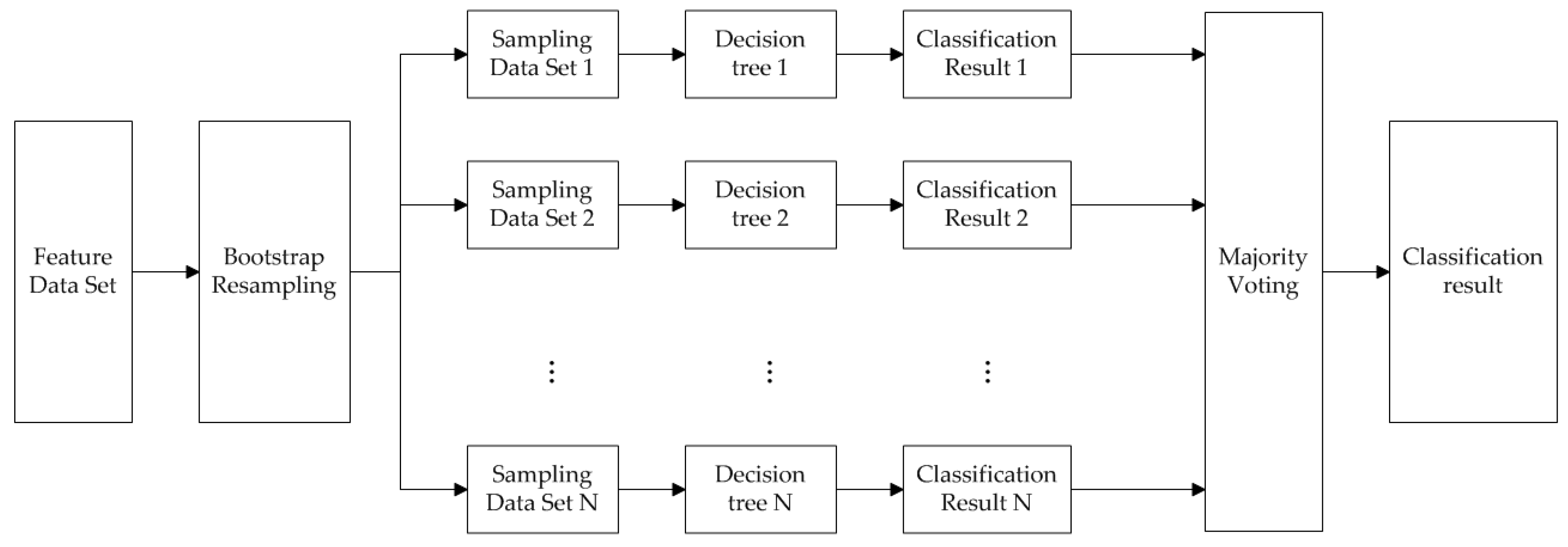
Relative entropy is an asymmetric measure of the difference between probabilities’ distributions. It is also known as Kullback–Leibler divergence (KLD), or information divergence. The relative entropy is equivalent to the difference in the information entropy of two probability distributions [21,22,23]. The band magnitude spectrum relative entropy is defined as follows:

$$E_{Rmag}(P\Vert Q)={\displaystyle \sum _{l=1}^L{P}_b(l)\times \log (\frac{P_b(l)}{Q_{b+1}(l)})}$$

(9)

$$H_{Rmag}(fr)=\frac{E_{Rmag}(b)}{{\log }_{2}L}$$

(10)

$$R{E}_{mag}(b)=\frac{1}{N_f}{\displaystyle \sum _{fr=1}^{N_f}{H}_{Rmag}(fr)}$$

(11)

Relative entropy was obtained by normalizing $E_{Rmag}$. It can measure the distance between two random distributions. The value of the relative entropy is zero when the corresponding random tests have the same distributions, and it increases with the increase in the two random distributions. Therefore, it can be used to compare the similarities between adjacent band signals.

The features of band magnitude spectrum entropy, band magnitude spectrum cross entropy, and band magnitude spectrum relative entropy are combined to form a signal magnitude spectrum entropy-based feature $F_m$, which is denoted as:

$$F_m=[B{E}_{mag},R{E}_{mag},C{E}_{mag}]$$

(12)

2.2. RF Model

RF is an ensemble learning method based on bagging. The accuracy and generalization performance of the model can be improved by combining multiple weak classifiers and majority voting. The structure of the RF model is shown in Figure 1. Through the random selection of data and features, the model improves the anti-noise ability of the algorithm. RF is a machine learning algorithm with strong generalization ability and flexibility. The prediction process is simple; it occurs through multiple rounds of numerical comparison operations [24,25,26]. This model has been used in cochlear implants because it can meet the real-time requirements of the hearing aid system.

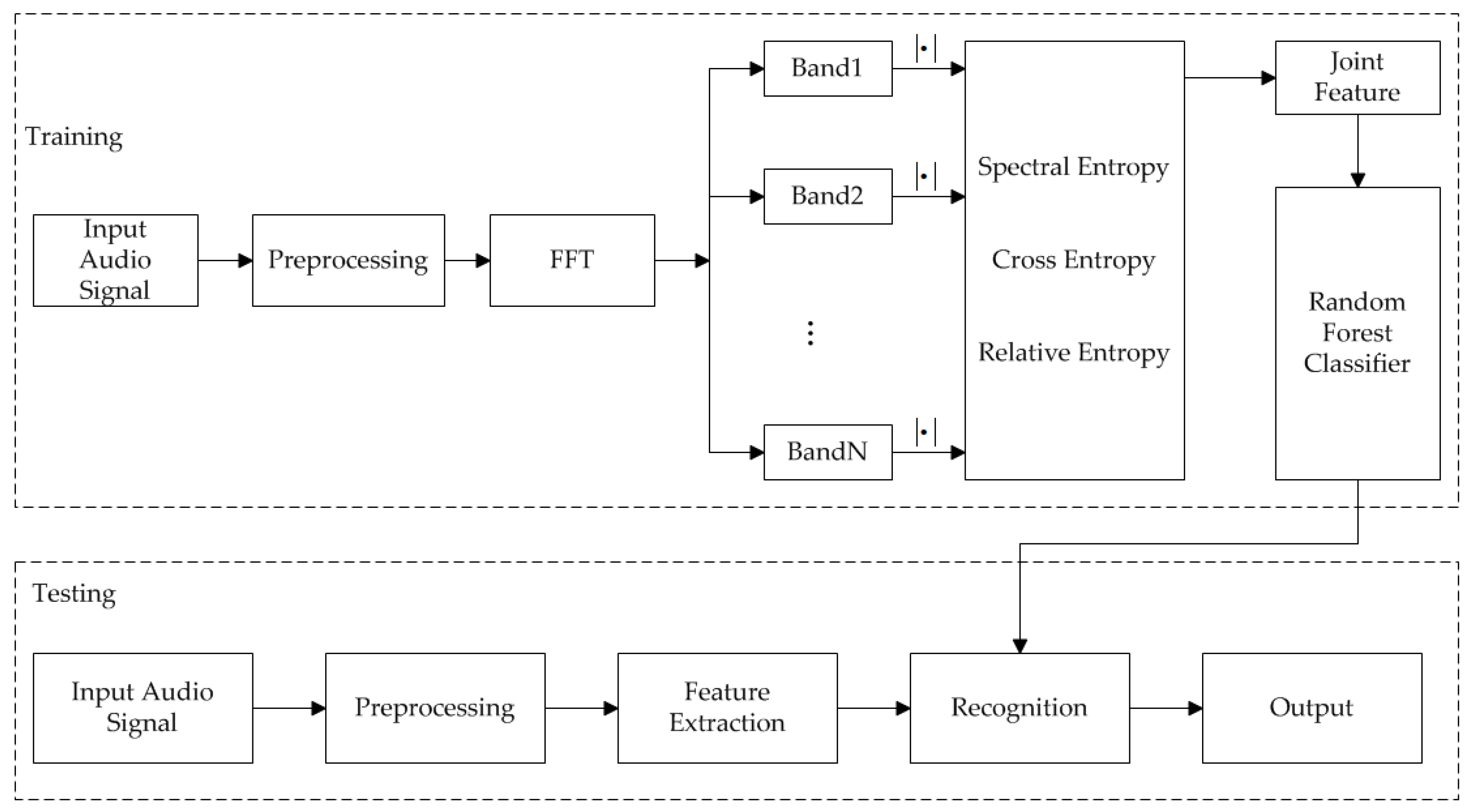
2.3. SEM-RF Algorithm

The implementation of audio classification for hearing aids using the SEM-RF algorithm is shown in Figure 2. The audio classification system consisted of model training and prediction. During model training, audio signal preprocessing and fast Fourier transform (FFT) are the first steps. Subsequently, feature extraction and dataset construction are completed. Finally, the features are applied to train the RF model. During model prediction, the corresponding features are extracted from the audio clips, and the trained model is used to obtain the classification results.

3. Robust Multi-MP Feature

In application environments containing speech signals, mutual interference between speech and background noise affects the stability of the classification features. Generally, the VAD algorithm is used to detect audio signal paragraphs containing speech and pure background noise. Subsequently, the background noise paragraph is classified by the trained model. The classification results depend on the accuracy of the VAD algorithm, and the use of the VAD algorithm also causes a time delay because it is usually not able to track the environment changes immediately [27]. This is especially true for environments that contain continuous speech signals. Robust features can improve the performance of the algorithm. Therefore, a multi-time resolution fusion feature based on magnitude and phase entropy features is proposed to improve the performance of the audio classification algorithm in the case of speech interference. Robust multi-time resolution fusion features can be directly used for audio classification to improve the classification accuracy of a speech-interferenced environment.

3.1. Magnitude Phase Features

The frequency spectrum can be divided into the magnitude and phase spectra. Phase spectrum information is often considered not important and it is ignored during speech signal processing [28]. Paraskevas et al. proved that the combination of magnitude spectrum features and phase features yields better classification results than the magnitude spectrum features, and they demonstrated the complementary nature of magnitude and phase [29]. Therefore, band phase spectrum features are introduced to form magnitude-phase band features with magnitude features. The corresponding band phase spectrum feature, band phase spectrum entropy, band phase spectrum cross entropy, and band phase spectrum relative entropy are as follows:

$$P_b(l)=\frac{{(phase(F_b(l)))}^2}{{\displaystyle \sum _{l=1}^L{(phase(F_b(l)))}^2}}$$

(13)

$$E_{phase}(b)=-{\displaystyle \sum _{l=1}^L{P}_b(l)\times lo{g}_2(P_b(l))}$$

(14)

$$H_{phase}(fr)=\frac{E_{phase}(b)}{lo{g}_{2}L}$$

(15)

$$B{E}_{phase}(b)=\frac{1}{N_f}{\displaystyle \sum _{fr=1}^{N_f}{H}_{phase}(fr)}$$

(16)

where $phase(\cdot )$ is the FFT phase spectrum of the signal.

$$Q_{b+1}(l)=\frac{{(\mathit{phase}(F_{b+1}(l)))}^2}{{\displaystyle \sum _{l=1}^L{(\mathit{phase}(F_{b+1}(l)))}^2}}$$

(17)

$$E_{Cphase}(P,Q)={\displaystyle \sum _{l=1}^L{P}_b(l)\times log(\frac{1}{Q_{b+1}(l)})}$$

(18)

$$H_{Cphase}(fr)=\frac{E_{Cphase}(b)}{lo{g}_{2}L}$$

(19)

$$C{E}_{phase}(b)=\frac{1}{N_f}{\displaystyle \sum _{fr=1}^{N_f}{H}_{Cphase}(fr)}$$

(20)

$$E_{Rphase}(P\Vert Q)={\displaystyle \sum _{l=1}^L{P}_b(l)\times log(\frac{P_b(l)}{Q_{b+1}(l)})}$$

(21)

$$H_{Rphase}(fr)=\frac{E_{Rphase}(b)}{lo{g}_{2}L}$$

(22)

$$R{E}_{phase}(b)=\frac{1}{N_f}{\displaystyle \sum _{fr=1}^{N_f}{H}_{Rphase}(fr)}$$

(23)

where $B{E}_{phase}$, $C{E}_{phase}$, $R{E}_{phase}$ are the corresponding band phase spectrum features.

The signal band entropy, band cross entropy, and band relative entropy features of the phase spectrum are joined to form the phase spectrum entropy-based feature, $F_p$.

$$F_p=[B{E}_{phase},R{E}_{phase},C{E}_{phase}]$$

(24)

$F_p$ and magnitude spectrum entropy-based feature constitute the magnitude-phase feature to take advantage of their complementary nature. Compared with magnitude feature, the magnitude phase feature has more comprehensive representation ability. The magnitude phase feature is expressed as follows:

$$F_{mp}=[F_m,F_p]$$

(25)

3.2. Multi-Time Resolution Fusion Feature

The feature extraction of the audio signal needs to separate the original audio into a continuous frame signal. During the separation of the audio signal, the frame length must be sufficiently short to ensure the stability of the signal and it must be long enough to preserve adequate frequency components [30] Subsequently, the FFT is adopted to obtain the frequency spectrum. During FFT, the time resolution declines with an increase in the window function length, whereas the frequency resolution increases. The sampling frequency of the audio signal we used in the experiment was 16 kHz. For feature extraction from a 25 ms frame length, there were 400 points in each signal frame. Subsequently, a 512 point FFT was applied for every signal frame. The frequency resolution of the spectrum is 16,000/512. For feature extraction from a 50 ms frame length, there are 800 points in each signal frame. Accordingly, a 1024 point FFT was applied for every signal frame. The frequency resolution of the spectrum is 16,000/1024. From the analysis, we observed that for signals with a 25 ms frame length, signal information can be obtained every 25 ms. However, the frequency information for every 16,000/512 Hz can be obtained. For signals with a 50 ms frame length, signal information can be obtained every 50 ms. However, frequency information for every 16,000/1024 Hz can be obtained. It was observed that signals divided by short frame length retain detailed information in the time domain compared with signals divided by a long frame length. Signals divided by long frame length retain detailed information in the frequency domain compared to those divided by a short frame length. Additionally, the features extracted from these frames can retain the corresponding information. Therefore, features of short-term frame signals can reflect the time characteristics in detail, and features of the long-term frame signal contain more frequency components [31] Feature extraction from different frame lengths considers the auditory system to receive acoustic signals on different dimensions. The multi-time resolution fusion feature maintains the sensitivity of different information and retains the representation ability of features in both the time and frequency domains.

During multi-time resolution fusion feature extraction, the audio signal is first framed into short paragraphs with different window lengths. Next, the band magnitude spectrum features and band phase spectrum features are extracted in each frame with different frame lengths. Finally, different time resolution features are fused to form the classification features. It is assumed that the band feature of the k-th ($k=1,2\cdots K$) frame length is $F_{mp\_res}(k)$; next, the multi-time resolution fusion feature $F_{mp\_mul}$ is represented as:

$$F_{mp\_mul}=[F_{mp\_res}(1),F_{mp\_res}(2),\cdots ,F_{mp\_res}(k),\cdots F_{mp\_res}(K)]$$

(26)

A multi-time resolution fusion feature extraction flowchart is shown in Figure 3. The process contains signal framing, Fourier transform, band feature extraction, and fusion. The length of the frame adopted in this study was 25 ms, 50 ms, 100 ms, and 200 ms respectively. Features extracted from frames of different lengths were combined into multi-time resolution fusion features.

4. ImSEM-RF

The combination of different features can improve classification accuracy. However, feature fusion causes the problem of dimension growth. An increase in the feature dimension significantly affects the speed of the model training and prediction. The algorithm in hearing aid applications has limitations in terms of speed implementation. To reduce the time complexity of model training and prediction, as well as to improve the calculation speed and efficiency, an LDA-RF classification model is proposed. The LDA-RF model is an improved RF algorithm based on LDA. High-dimensional features are converted into simple features to increase the speed of model training and prediction. The ImSEM-RF algorithm applies a robust multi-MP feature and LDA-RF classification model to improve the performance of mixed speech environments.

4.1. LDA

LDA achieves data dimension reduction using supervised learning. For the input audio feature datasets F_DS,

$$F\_DS=\left\{(f_{mp\_mul1},y_1),(f_{mp\_mul2},y_2),\cdots (f_{mp\_mulm},y_m)\right\}$$

(27)

where $f_{mp\_mul}$ is the d-dimensional audio signal feature and $y$ corresponds to the feature label. The sample number of the j-th class is $N_j(j=1,2,\cdots J)$. $F_j(j=1,2,LJ)$ is the sample collection of the j-th class. ${\mu }_j(j=1,2,\cdots J)$ is the mean vector and ${\Sigma }_j(j=1,2,\cdots J)$ represents the covariance matrix. Suppose the dimension of the low-dimensional space is $d_L$. The corresponding basis vector is $(w_1,w_2,\cdots w_d)$. The matrix W is composed of a basis vector.

The within-class scatter matrix $S_w$ is expressed as:

$$S_w={\displaystyle \sum _{j=1}^J{S}_{wj}={\displaystyle \sum _{j=1}^J{\displaystyle \sum _{f_{mp\_mul}\in F_j}^{}(f_{mp\_mul}-{\mu }_j){(f_{mp\_mul}-{\mu }_j)}^T}}}$$

(28)

The between-class scatter matrix $S_b$ is expressed as:

$$S_b={\displaystyle \sum _{j=1}^J{N}_j({\mu }_j-\mu )}{({\mu }_j-\mu )}^T$$

(29)

where $\mu$ is the mean vector for all the samples. By maximizing the between-class scatter matrix and minimizing the within-class scatter matrix, the objective function is optimized, and the corresponding projection matrix W is derived.

$$J(w)=\frac{W^T{S}_{b}W}{W^T{S}_{w}W}$$

(30)

Each of the samples in the dataset is converted to a new sample by multiplying the transposed matrix W^T, namely $f{l}_i=W^T{f}_{mp\_muli}$. $fl$ is the corresponding low-dimensional feature. High-dimensional features are converted to low-dimensional features to accelerate the model training and prediction process [32,33,34].

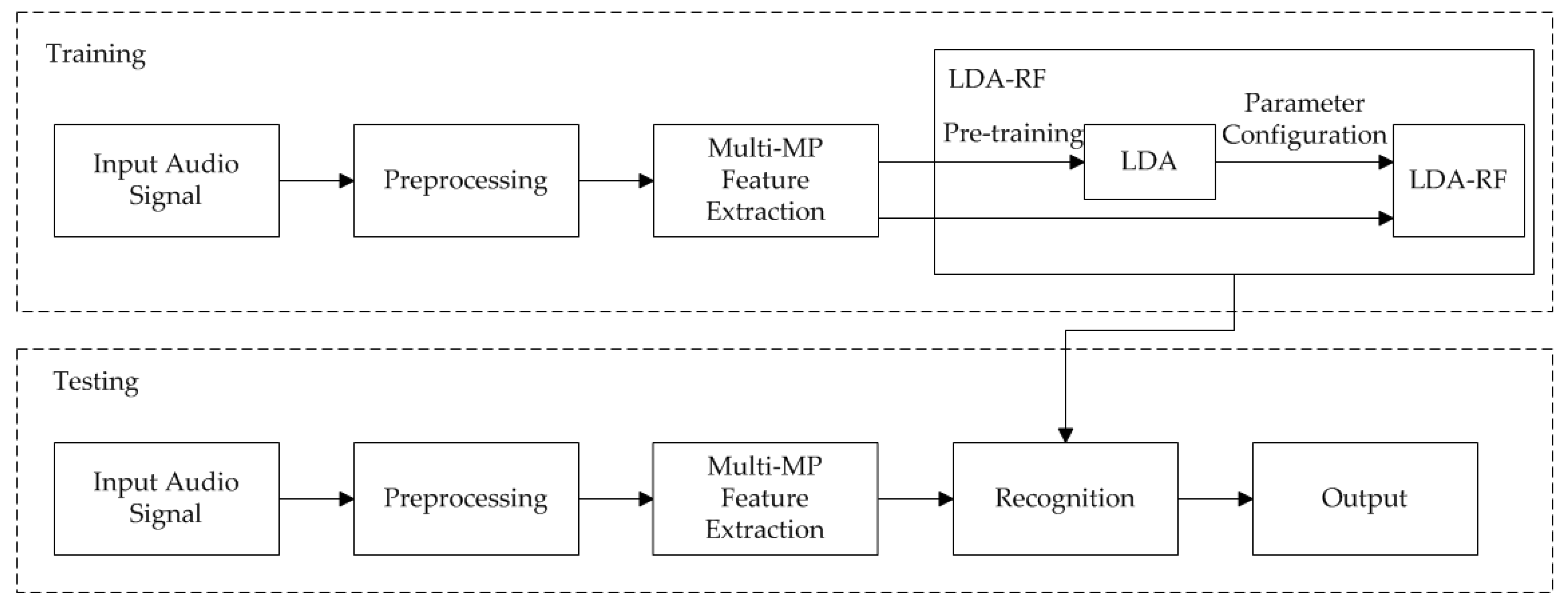
4.2. ImSEM-RF Algorithm

During audio classification, the dimension of the magnitude spectrum band feature and phase spectrum band feature is d. Features of K resolutions are adopted. Subsequently, the dimensions of the final classification feature are 2d $\times$ K. The data change in the feature matrix not only introduces more redundant information and noise, but also results in an increased computation in the calculation. Thus, the model classification speed was affected. Therefore, to address the problem of classification speed for high-dimensional features, RF was improved by adding a linear discriminant analysis module. The LDA-RF model can accelerate the process of training and prediction by removing redundant feature information and noise.

The implementation of the ImSEM-RF algorithm is shown in Figure 4. The audio classification system consisted of model training and prediction. During model training, the input audio signal is first divided by different frame lengths. Next, the magnitude and phase features are extracted for different frame lengths. The frame lengths used in this study were 25, 50, 100, and 200 ms. The features were combined to represent the signal. We used high-dimensional features to train the LDA model. Subsequently, low-dimensional features were obtained by pre-training the LDA model. Low-dimensional features were applied to the RF model training. Subsequently, the complete LDA-RF model was obtained. During prediction, the corresponding features are extracted on different frame lengths, and the trained model is used to obtain the classification results. Compared with the SEM-RF method, multi-MP feature extraction is applied to improve the robustness of the feature and the RF model is improved by LDA to achieve acceleration for high-dimensional features.

5. Experimental Results

The dataset and experimental results are presented here. First, a hearing aid research dataset for acoustic environment recognition is introduced. Next, the parameter configuration of the feature extraction and classification model is presented. Finally, the audio classification result of the SEM-RF algorithm is compared with the background noise classification algorithm in [12] In addition, the robustness of the multi-time resolution magnitude-phase feature was verified using experiments, and the acceleration effect of the LDA-RF model is demonstrated. The mixed-speech audio classification results of the ImSEM-RF algorithm are presented in terms of both the accuracy improvement of robust features and speed acceleration in the classification model.

5.1. Data Set

The experimental data were obtained from the hearing aid research dataset for acoustic environment recognition [17], open-sourced by the Center of Competence for Hearing Systems in Germany. The dataset provided audio signals recorded in different acoustic environments. Background audio signals and speech in background audio signals were applied to the experiments. Background audio signals contain seven common environments: cocktail party, traffic, vehicle, music, quiet indoors, reverberant environment and wind turbulence. Because the background noise in cocktail party consisted of speech signals, the remaining six environments were mixed with speech signals to form speech in the background audio signal. Each set of audio signals contained content received by the left and right ears. The signal sample rate was 16,000 Hz. The signal fragment duration was 10 s. The background audio signals from the seven environments contained 4556 sets of binaural data, and 9112 clips. The speech in the background audio signals from six environments contained 62,835 sets of binaural data, and 125,670 clips in total. The cocktail party was removed when constructing speech in the background audio signal because of the speech characteristics. After data cleaning, 80% of the data were used to train the classification model, and the remaining data were used to test the trained model.

5.2. Experimental Setup

The algorithm [12] based on band periodicity, band entropy feature, and RF model proved to be effective. The parameter configuration in the feature extraction and model training is consistent with the configuration in this study. During the framing process, the frame length was 25 ms and the overlap between adjacent frames was 0. The audio signal was divided into eight bands in the frequency domain. The center frequencies of the sub-bands were 500, 1500, 2500, 3500, 4500, 5500, 6500, and 7500 Hz. The bandwidth of the sub-bands was 1000 Hz. The periodicity features in all eight bands and the entropy features in all eight bands were joined to form a classification feature. Fifty estimators were used in the RF model.

The parameter configuration of the SEM-RF algorithm is as follows. The signal spectrum was divided into eight bands in the frequency domain during spectrum entropy information feature extraction. The center frequencies of the sub-bands were 500, 1500, 2500, 3500, 4500, 5500, 6500, and 7500 Hz. The bandwidth of the sub-bands was 1000 Hz. Seven band magnitude spectrum cross entropy, seven band magnitude spectrum relative entropy, and eight band magnitude spectrum entropy features were adopted to form the classification feature. Fifty estimators were applied to the RF classifier.

The parameter configuration of the ImSEM-RF algorithm is as follows. During the extraction of multi-time resolution fusion features based on magnitude and phase spectrum entropy information, a frame length of four time resolutions was adopted, and the overlap between adjacent frames was 0. The frame lengths were 25, 50, 100, and 200 ms. During the extraction of magnitude phase features, the corresponding phase spectrum feature, band phase spectrum entropy, band phase spectrum cross entropy, and band phase spectrum relative entropy were combined with the magnitude spectrum features. The other basic parameter configuration was the same as that of the SEM-RF algorithm. The high-dimensional multi-time resolution fusion feature was projected onto a five-dimensional space using the linear discriminant analysis module in the LDA-RF model. Fifty estimators were applied to the RF classifier. Before training and testing the model, the missing and abnormal values were filtered out to remove the exception feature vector in the dataset. In addition, the dataset contained two channels of audio signals. Therefore, features $F_l$ and $F_r$ extracted from the left ear and right ear channels were joined according to the method given in [35], namely $F=[F_l,F_r]$.

5.3. Experimental Results

5.3.1. SEM-RF Classification Results

The band magnitude spectrum entropy, band magnitude spectrum cross entropy, and band magnitude spectrum relative entropy features were extracted from seven types of background environment to form the band magnitude spectrum entropy information-based feature. The RF model was adopted to train and test the dataset. The experimental SEM-RF results were compared with the algorithm in [12], denoted as P&E RF.

Table 1. Comparison of the classification results of the background audio signal dataset.

	In Traffic	In Vehicle	Music	Quiet Indoors	Rever- Berant	Wind	Cocktail Party	Test Set
P&E RF	89.22%	96.15%	97.60%	91.09%	52.86%	89.86%	92.37%	90.99%
SEM-RF	100.00%	99.17%	99.69%	95.96%	79.59%	97.94%	96.80%	97.58%

summarizes the classification results for the seven different background environments, including the classification accuracy for every environment and for the test set. The experimental results indicate that the proposed feature based on entropy information significantly improves the accuracy of the classification algorithm. The classification accuracy in each environment was improved, especially in traffic and reverberant environments. Classification accuracies of approximately 10% and 27% increased. The classification accuracy increased by approximately 7% on the entire background audio signal test set. For some types of audio signal, significant differences in the time domain were observed. For example, an indoor environment can be quiet with sudden, small perturbations, such as appliances turning on. For some types of audio signal, there are significant differences in the frequency domain compared to the time domain. For example, white noise [36] is a random signal featuring equal intensity at different frequencies, giving it a constant-power spectral density. Pink noise or 1/f noise is a signal with a frequency spectrum such that the power spectral density is inversely proportional to the frequency of the signal. White noise is commonly used in the production of electronic music. Pink noise is one of the most common signals in biological systems [37]. These two types of noise have obvious differences in frequency domain. However, the band periodicity and band entropy features mainly show the time domain characteristics of the audio signals. The SEM features mainly demonstrate the frequency domain characteristics of the audio signals. The multi-MP feature demonstrates both the frequency and time domain characteristics of the audio signals. For signals with obvious differences in the frequency domain, these features can improve the classification performance. In addition, the signals have different distributions in the frequency domain. Based on band cross entropy and band relative entropy features, the similar and different characteristics of the probability distribution of adjacent sub-bands can be used to distinguish audio signals. Additionally, the relation between adjacent frequency spectrum sub-band probability distributions is an important property for classification. The SEM feature takes advantage of the characteristics of each sub-band and the relation of adjacent sub-band probability distribution at the same time, which improves the representation ability of the audio signals. The reverberant environment is mainly confused with the cocktail party and music. On one hand, in both environments, the cocktail party and reverberant environment, there are reverberations involved. On the other hand, the reverberant environment dataset has the least amount of data. Owing to the small amount of data, the classification model cannot learn enough information. An unbalanced amount of data also makes the classification accuracy of the reverberant environment significantly lower than that of other environments.

5.3.2. ImSEM-RF Classification Results

Although the audio classification algorithm based on the band magnitude spectrum entropy information feature achieves excellent classification accuracy in background audio signals, there is a significant decline in classification results when the audio signal is affected by speech. The experimental results of the band magnitude spectrum entropy information feature in the mixed-speech environments, denoted as the SEM feature, are summarized in

Table 2. Comparison of classification results of the features extracted from speech in background audio signal dataset.

	In Traffic	In Vehicle	Music	Quiet Indoors	Rever- Berant	Wind	Test Set
SEM feature	89.65%	91.11%	97.13%	95.42%	82.81%	88.50%	91.83%
MP joint feature	90.51%	91.30%	98.22%	96.41%	82.62%	89.53%	92.55%
Multi-MP feature	91.80%	94.24%	99.02%	97.25%	85.52%	93.23%	94.42%

. Compared with the background audio signal classification results, the classification accuracy of the mixed-speech environment decreased by approximately 6%. The experimental results of the magnitude phase feature and multi-time resolution fusion feature are also summarized in Table 2, denoted as MP joint feature and multi-MP feature, respectively. An RF classifier with 50 estimators was used to test the stability of the MP joint feature and multi-MP feature.

The experimental results of the MP joint feature indicate that the classification accuracy is improved in all audio scenes except for the reverberant environment compared with the SEM feature. The classification accuracy of the reverberant environment only decreased by approximately 0.2%. Therefore, the magnitude phase spectrum feature can enhance the stability of the signal feature, in accordance with its complementary nature. The multi-time resolution fusion feature improves the classification accuracy in all environments. Compared with the magnitude spectrum feature using only one time resolution, the classification accuracy of the multi-time resolution fusion features using the test set increases by approximately 2.6%. The experimental results indicate that the multi-time resolution magnitude phase feature can effectively improve the classification accuracy of background audio signal environments affected by speech.

The experimental results of the ImSEM-RF algorithm are summarized in

Table 3. Comparison of the classification results of the improved algorithm.

	In Traffic	In Vehicle	Music	Quiet Indoors	Rever- Berant	Wind	Test Set
Multi-MP-RF	91.80%	94.24%	99.02%	97.25%	85.52%	93.23%	94.42%
ImSEM-RF	88.43%	94.05%	98.07%	94.05%	88.96%	93.28%	93.92%

. Based on the multi-time resolution fusion feature dataset, the program running time of classification model training and prediction with different numbers of estimators is demonstrated in Figure 5. The classification results of multi-MP features using the LDA-RF classification model, denoted as ImSEM-RF, are compared with those of multi-MP features using the RF classification model, denoted as multi-MP-RF, to demonstrate the effectiveness of the LDA-RF model.

The experimental results indicate that the classification accuracy of the LDA-RF model decreases by less than 1% compared with that of the RF model using the test set. However, the speed of the model training and prediction significantly improves. When the number of estimators increases from 50 to 1000, the overall program running time information, including data import, dataset split, model training and prediction, and other processes using Python on an Intel i7 8th gen laptop are given. The proportion of the overall program running time of the LDA-RF/RF decreases from approximately 20% to 10%. The LDA-RF model can effectively accelerate the classification speed of complex models while maintaining improved accuracy compared with the RF classification model.

6. Conclusions

In this study, we present SEM-RF for background audio classification and ImSEM-RF for mixed-speech environment classification for hearing aids. The main goal of these methods is to improve the stability of the audio signal features and increase the classification accuracy. First, a novel-feature SEM based on similarity and stability was introduced to improve the classification of each audio environment. Next, the SEM features and corresponding phase features were fused on multiple time resolutions to form a multi-MP feature to improve the robustness of the signal representation. Finally, the random forest model was improved by the linear discriminant analysis method to form the LDA-RF classification model, which achieves model acceleration. The experimental results indicate that the proposed SEM-RF algorithm increases the classification accuracy by approximately 7% compared with the background noise classification algorithm using a random forest tree classifier with band periodicity and band entropy features. The proposed ImSEM-RF algorithm increases the classification accuracy by approximately 2% compared with the SEM-RF algorithm for speech-interferenced environment. The proposed algorithms provide accurate classification of background audio signals and speech-interferenced audio signals.

Limited computational resources in hearing aids pose challenges to machine learning systems. Therefore, we implemented the SEM-RF algorithm and ImSEM-RF algorithm on an Intel core i7 8th gen laptop to estimate the computational demands. We used MATLAB to perform the feature extraction and Python to perform the model training and prediction. The main process in SEM-RF algorithm takes less than 0.5 s for every 10 s of audio signal. The main process in the ImSEM-RF algorithm takes less than 2 s for every 10 s of audio signal. The feature extraction process takes up most of the time. The optimization of computational resources is yet to be developed by researchers for real-time applications.

References

1. Gerlach, L.; Payá-Vayá, G.; Blume, H. A Survey on Application Specific Processor Architectures for Digital Hearing Aids. J. Signal Process. Syst. 2021, 1–16. [Google Scholar] [CrossRef]
2. Kates, J.M. Digital Hearing Aids; Plural Publishing: San Diego, CA, USA, 2008. [Google Scholar]
3. Pandey, A.; Mathews, V.J. Low-Delay Signal Processing for Digital Hearing Aids. IEEE Trans. Audio Speech Lang. Process. 2010, 19, 699–710. [Google Scholar] [CrossRef]
4. Alexandre, E.; Cuadra, L.; Gil-Pita, R. Sound Classification in Hearing Aids by the Harmony Search Algorithm; Springer: Berlin/Heidelberg, Germany, 2009; Volume 191, pp. 173–188. [Google Scholar] [CrossRef]
5. Alexandre, E.; Cuadra, L.; Alvarez, L.; Rosa-Zurera, M. NN-based automatic sound classifier for digital hearing aids. In Proceedings of the 2007 IEEE International Symposium on Intelligent Signal Processing, Xiamen, China, 28 November–1 December 2007; pp. 1–6. [Google Scholar] [CrossRef]
6. Tanweer, S.; Mobin, A.; Alam, A. Environmental Noise Classification using LDA, QDA and ANN Methods. Indian J. Sci. Technol. 2016, 9, 1–8. [Google Scholar] [CrossRef]
7. Liu, T.; Yan, D.; Wang, R.; Yan, N.; Chen, G. Identification of Fake Stereo Audio Using SVM and CNN. Information 2021, 12, 263. [Google Scholar] [CrossRef]
8. Barkana, B.D.; Saricicek, I. Environmental Noise Source Classification Using Neural Networks. In Proceedings of the 2010 Seventh International Conference on Information Technology: New Generations, Washington, DC, USA, 12–14 April 2010; pp. 259–263. [Google Scholar] [CrossRef]
9. Nordqvist, P.; Leijon, A. An efficient robust sound classification algorithm for hearing aids. J. Acoust. Soc. Am. 2004, 115, 3033–3041. [Google Scholar] [CrossRef] [PubMed]
10. Büchler, M.; Allegro, S.; Launer, S.; Dillier, N. Sound Classification in Hearing Aids Inspired by Auditory Scene Analysis. EURASIP J. Adv. Signal Process. 2005, 2005, 387845. [Google Scholar] [CrossRef] [Green Version]
11. Lamarche, L.; Giguère, C.; Gueaieb, W.; Aboulnasr, T.; Othman, H. Adaptive environment classification system for hearing aids. J. Acoust. Soc. Am. 2010, 127, 3124–3135. [Google Scholar] [CrossRef] [PubMed]
12. Saki, F.; Kehtarnavaz, N. Background noise classification using random forest tree classifier for cochlear implant applications. In Proceedings of the 2014 IEEE International Conference on Acoustics, Speech and Signal Processing (ICASSP), Florence, Italy, 4–9 May 2014; pp. 3591–3595. [Google Scholar] [CrossRef]
13. Saki, F.; Sehgal, A.; Panahi, I.; Kehtarnavaz, N. Smartphone-based real-time classification of noise signals using subband features and random forest classifier. In Proceedings of the 2016 IEEE International Conference on Acoustics, Speech and Signal Processing (ICASSP), Shanghai, China, 20–25 March 2016; pp. 2204–2208. [Google Scholar] [CrossRef]
14. Alavi, Z.; Azimi, B. Application of Environment Noise Classification towards Sound Recognition for Cochlear Implant Users. In Proceedings of the 2019 6th International Conference on Electrical and Electronics Engineering (ICEEE), Istanbul, Turkey, 16–17 April 2019; pp. 144–148. [Google Scholar] [CrossRef]
15. Saki, F.; Kehtarnavaz, N. Automatic switching between noise classification and speech enhancement for hearing aid devices. In Proceedings of the 2016 38th Annual International Conference of the IEEE Engineering in Medicine and Biology Society (EMBC), Orlando, FL, USA, 16–20 August 2016; pp. 736–739. [Google Scholar] [CrossRef]
16. Alamdari, N.; Kehtarnavaz, N. A Real-Time Smartphone App for Unsupervised Noise Classification in Realistic Audio Environments. In Proceedings of the 2019 IEEE International Conference on Consumer Electronics (ICCE), Las Vegas, NV, USA, 11–13 January 2019; pp. 1–5. [Google Scholar] [CrossRef]
17. Hüwel, A.; Adiloğlu, K.; Bach, J.-H. Hearing aid Research Data Set for Acoustic Environment Recognition. In Proceedings of the ICASSP 2020—2020 IEEE International Conference on Acoustics, Speech and Signal Processing (ICASSP), Barcelona, Spain, 4–8 May 2020; pp. 706–710. [Google Scholar] [CrossRef]
18. Yuxin, Z.; Yan, D. A voice activity detection algorithm based on spectral entropy analysis of sub-frequency band. BioTechnol. Indian J. 2014, 10, 12342–12348. [Google Scholar]
19. Powell, G.E.; Percival, I.C. A spectral entropy method for distinguishing regular and irregular motion of Hamiltonian systems. J. Phys. A Math. Gen. 1979, 12, 2053–2071. [Google Scholar] [CrossRef]
20. Chen, X.; Kar, S.; Ralescu, D.A. Cross-entropy measure of uncertain variables. Inf. Sci. 2012, 201, 53–60. [Google Scholar] [CrossRef]
21. Kullback, S.; Leibler, R.A. On information and sufficiency. Ann. Math. Stat. 1951, 22, 79–86. [Google Scholar] [CrossRef]
22. Goodfellow, I.; Bengio, Y.; Courville, A. Deep Learning; MIT Press: Cambridge, UK, 2016; Volume 1, pp. 71–73. [Google Scholar]
23. Polykovskiy, D.; Novikov, A. Bayesian Methods for Machine Learning. Coursera and National Research University Higher School of Economics. 2018. Available online: https://www.hse.ru/en/edu/courses/220780748 (accessed on 10 October 2021).
24. Breiman, L. Random forests. Mach. Learn. 2001, 45, 5–32. [Google Scholar] [CrossRef] [Green Version]
25. Cutler, A.; Cutler, D.R.; Stevens, J.R. Random forests. In Ensemble Machine Learning; Springer: Boston, MA, USA, 2012; pp. 157–175. [Google Scholar] [CrossRef]
26. Biau, G. Analysis of a random forests model. J. Mach. Learn. Res. 2012, 13, 1063–1095. [Google Scholar]
27. Loizou, P.C. Speech Enhancement: Theory and Practice; CRC Press: Boca Raton, FL, USA, 2007. [Google Scholar] [CrossRef]
28. Wang, D.; Lim, J. The unimportance of phase in speech enhancement. IEEE Trans. Acoust. Speech Signal Process. 1982, 30, 679–681. [Google Scholar] [CrossRef]
29. Paraskevas, I.; Chilton, E. Combination of magnitude and phase statistical features for audio classification. Acoust. Res. Lett. Online 2004, 5, 111–117. [Google Scholar] [CrossRef]
30. Owens, F.J. Signal Processing of Speech; Macmillan International Higher Education: London, UK, 1993. [Google Scholar]
31. Orfanidis, S.J. Introduction to Signal Processing; Pearson Education, Inc.: Boston, MA, USA, 2016. [Google Scholar]
32. Balakrishnama, S.; Ganapathiraju, A. Linear discriminant analysis-a brief tutorial. Inst. Signal Inf. Processing 1998, 18, 1–8. [Google Scholar]
33. Xanthopoulos, P.; Pardalos, P.M.; Trafalis, T.B. Linear discriminant analysis. In Robust Data Mining; Springer: New York, NY, USA, 2013; pp. 27–33. [Google Scholar] [CrossRef]
34. Tharwat, A.; Gaber, T.; Ibrahim, A.; Hassanien, A.E. Linear discriminant analysis: A detailed tutorial. AI Commun. 2017, 30, 169–190. [Google Scholar] [CrossRef] [Green Version]
35. Mirzahasanloo, T.; Kehtarnavaz, N. Real-time dual-microphone noise classification for environment-adaptive pipelines of cochlear implants. In Proceedings of the 2013 35th Annual International Conference of the IEEE Engineering in Medicine and Biology Society (EMBC), Osaka, Japan, 3–7 July 2013; pp. 5287–5290. [Google Scholar] [CrossRef]
36. Mancini, R.; Carter, B. Op Amps for Everyone; Texas Instruments: Dallas, TX, USA, 2009; pp. 10–11. [Google Scholar]
37. Szendro, P.; Vincze, G.; Szasz, A. Pink-noise behaviour of biosystems. Eur. Biophys. J. 2001, 30, 227–231. [Google Scholar] [CrossRef]
Figure 1. RF classification model.
Information 13 00079 g001
Figure 2. Implementation of audio classification for hearing aids using the SEM-RF algorithm.
Information 13 00079 g002
Figure 3. Flow chart of multi-time resolution fusion feature extraction.
Information 13 00079 g003
Figure 4. Implementation of the ImSEM-RF algorithm.
Information 13 00079 g004
Figure 5. The experimental results of the LDA-RF classification model and the RF model tested on multi-time resolution fusion feature based on magnitude-phase feature. (a) Increasing program running time with increasing number of estimators. (b) The proportion of the program running time of the LDA-RF/RF with increasing numbers of estimators.
Information 13 00079 g005