HIL Flight Simulator for VTOL-UAV Pilot Training Using X-Plane

Abstract

With the increasing popularity of vertical take-off and landing unmanned aerial vehicles (VTOL UAVs), a new problem arises: pilot training. Most conventional pilot training simulators are designed for full-scale aircrafts, while most UAV simulators are just focused on conceptual testing and design validation. The X-Plane flight simulator was extended to include new functionalities such as complex wind dynamics, ground effect, and accurate real-time weather. A commercial HIL flight controller was coupled with a VTOL convertiplane UAV model to provide realistic flight control. A real flight case scenario was tested in simulation to show the importance of including an accurate wind model. The result is a complete simulation environment that has been successfully deployed for pilot training of the Marvin aircraft manufactured by FuVeX.

1. Introduction

An unmanned aerial vehicle (UAV) is often referred to as a remotely piloted aircraft or an unmanned aircraft that can be controlled with or without a human operator. Rotary wing UAVs such as quadcopters and hexacopters are widely used due to their low costs, simplicity, and hovering flight capabilities. The main downside of these vehicles is that their range is very limited, because all the lift required to overcome the UAV weight must be provided by the motors. Conventional fixed-wing UAVs allow for longer operations, but require a runway for take-off and landing. Vertical take-off and landing (VTOL) convertiplane UAVs combine the advantages of both aircraft types, allowing for vertical take-off, landing, and hovering capabilities with extended flight ranges. The increasing popularity of this type of UAVs has given rise to a new problem: UAV pilot training.

VTOL convertiplane UAVs (from now on, VTOL UAVs for simplicity) require very specific piloting skills, since pilots need to be able to control the vehicle both as an airplane and as a quadcopter. Traditional radio-controlled aircraft pilots often find it difficult to transition from airplane piloting to quadcopter piloting. The reverse is even more challenging. Conventional pilot training has traditionally been conducted in flight simulators, but transferring this technology to the training of VTOL UAV pilots in a simulator poses a series of challenges. For example, VTOL UAVs are extremely sensitive to wind disturbances during take-off, landing, and hovering phases. Throughout this paper we will demonstrate the progress made to develop a flight simulator capable of being used to train VTOL UAV pilots in different scenarios.

Section 2 contains a brief introduction to the state of the art in UAV flight simulation. Section 3 summarizes our contributions in this field. Section 4 is devoted to modeling the simulator for our specific aircraft: the Marvin VTOL UAV. The integration with X-Plane is explained in Section 5, and additional plugins such as live weather and ground effect are detailed in Section 6. Materials and methods are presented in Section 7. Section 8 gathers the results of the research and the operation of the fully-working simulator. Finally, conclusions are summarized in Section 9.

2. Related Works

The increasing popularity of electric VTOL UAVs due to their unique take-off and landing capabilities, coupled with longer ranges than rotary wing UAVs, has promoted numerous studies on the simulation of this type of aircraft over the last 20 years [1,2,3,4,5].

The typical simulation choice for computation is MATLAB [6,7], which offers full freedom to define the dynamics of the UAV. However, the complexity of having to derive the whole flight dynamics often incurs oversimplifications such as only considering front-wind aerodynamics [8], or very basic PID flight controllers [9]. Some more recent works relegate the calculation of the aircraft dynamics to a flight simulator such as RealFlight [10] or X-Plane [11,12]. Other robotics simulators such as Gazebo have also been employed for UAV simulation [13].

Using a flight simulator does not only offer the advantage of leveraging the flight dynamics computation to the internal physics engine of the simulator, but it also provides a more complex world model that otherwise would require too many hours of development: live-weather, 3D scenery, and elevation maps, day–night cycles, advanced visualization features, etc.

On the other hand, most of the cited works are focused on simulating a VTOL UAV for performance analysis and conceptual design, but few of them focus on pilot training or even consider the input of a pilot [14].

Flight simulators are a very established tool [15] for commercial and military pilots training [16,17]. When appropriately designed, it has been demonstrated that simulation can provide competence development with pedagogical and economic advantages [18].

The increasing trend of unmanned aerial platforms, and its consequent increase in the number of pilots, has emphasized the need for pilot training to prevent accidents and reduce operating costs. A survey on commercial and open-source unmanned vehicle simulators [19] concluded that it is no longer necessary to build a new simulator from scratch. Newer and/or specialized engines such as the flight simulator X-Plane or Ageia PhysX and Havok physics engines are perfectly capable of simulating complex physical interactions.

Another critical aspect in UAV flight simulation is the flight controller integration. A usual approach to this problem consists of running the flight controller code in the same computer where the flight simulation is performed. This digitalization of the flight controller is usually called software-in-the-loop (SITL) simulation. Many UAV simulators follow this approach [20,21,22]. However, running the same code in a virtual environment does not guarantee the same exact performance as running it in the actual flight controller hardware. For this reason, running the actual flight controller with its own specific hardware connected to the simulation environment can significantly reduce the risk and cost associated with experimental validation [23]. This next step is called hardware-in-the-loop (HIL or HITL) simulation.

Both SITL and HIL are addressed in the well-accepted V-model development approach for model-based design of embedded systems [24]. The V-model development process includes a series of steps to validate a product in increasingly complex and realistic testing conditions to provide proper feedback for design correction [25]. A detailed diagram of the V-model development process can be found in the literature [26].

In general, HIL simulation is considered the last step before prototype testing [23]. Therefore, the authors consider that it is the most reasonable simulation approach to help in the training of pilots.

HIL implementations of a VTOL UAV simulator are more scarce [27,28], and none of them consider weather conditions [12,29,30]. Another advantage of HIL simulation is that, by connecting the actual aircraft components to the flight controller, actual actuator outputs can be bench-tested [31].

3. Contributions

We developed a full-featured HIL solution of a commercial UAV-VTOL (Marvin aircraft, manufactured by FuVeX). The aircraft was modeled on X-Plane. Real behavior of the UAV was achieved via HIL integration, and weather conditions were obtained by our own integration of Active Sky (Active Sky website: https://hifisimtech.com/asxp/, accessed on 28 September 2022) data and X-Plane. A plugin was developed. This plugin takes Active Sky weather data as input, calculates the corresponding aerodynamic forces and moments of the aircraft in these conditions, and adds them back to the X-Plane physical model. The plugin ensures that the physical model of the aircraft considers the aerodynamic coefficients corresponding to the direction of the wind with respect to the aircraft body framework. To our knowledge, this approach is not considered in any other paper.

4. UAV-VTOL Modeling

Initially, a large amount of aircraft data has to be collected before proceeding to the model design in X-Plane. Firstly, the minimum model parts that must be present in the model should be specified. This particular UAV-VTOL is composed of a fixed wing and four motors in a quadcopter arrangement with a tilt mechanism. In quadcopter mode, all four engines are facing upwards. When transitioning to plane mode, the four arms are tilted down until all four motors point forward. The main components to be considered are:

• Wing and endplates.
• Fuselage (considering the airfoil shape).
• Engines and propellers.
• Connecting engine arms (carbon fiber rods) and tilt mechanism.
• Tail: vertical tail plane (VTP), horizontal tail plane (HTP), and the connecting carbon fiber rod.
• Basic landing gear.

Figure 1 shows a 3D render of the UAV-VTOL both in copter and plane mode, featuring all the minimum model parts for reference, except for the landing gear.

4.1. Mass, Inertia, and Geometric Data

The mass and inertia properties were collected via experimental weighting of components and CAD modules. The essential values to collect for the model are total weight, wingspan, length, center of gravity position ($x_{CG}$, $y_{CG}$, $z_{CG}$), tilt center position ($x_{tilt}$, $z_{tilt}$), and inertia values ($I_{xx}$, $I_{yy}$, $I_{zz}$, $I_{xy}$, $I_{xz}$, $I_{yz}$). Note that the $y_{tilt}$ component is neglected, assuming a reference system in which the Y axis denotes the distance to the mid-plane of the aircraft.

The relative position of each engine has to be specified as well, to match the flight controller setup. In this aircraft, the rear engine arms are displaced vertically 30 mm up from the mid-plane, while front engine arms are displaced 30 mm down from the mid-plane. The mid-plane offset occurs at the joint of the tilt mechanism, and connecting carbon rods are drawn as hollow rods of a certain diameter.

Other measurements, such as the tail rod length and ground clearance or landing gear height, must also be provided.

4.2. Aerodynamic Specifications

To properly reconstruct the wing and fuselage, many parameters have to be provided for each wing: chord (root and tip chord values if the wing is tapered), sweep angle, dihedral angle, wingspan, thickness, aerodynamic center ($x_{AC}$, $y_{AC}$, $z_{AC}$), position relative to the fuselage, and airfoil shape.

The 2D airfoil aerodynamic coefficient plots are indispensable to match the aerodynamic performance, as explained in Section 5. They can be obtained from CFD simulations, potential flow solvers such as XFoil [32], or airfoil databases such as Airfoil Tools.

Although it is not essential at this stage, it may also be of interest to collect aerodynamic data of the entire aircraft such as the coefficient of lift, drag, or moment for different angles of attack for model validation and tweaking. In any case, these values will be essential for implementing the wind plugin in Section 6.

Control Surfaces

Only two control surfaces are available in this aircraft: elevator and rudder. Attitude changes use the help of differential thrust/mixing between the four motors. Both the elevator and the rudder are actuated by independent servos, with a maximum and minimum deflection of (±30 degrees). In this case, the entire vertical tail plane (VTP) and horizontal tail planes (HTP) act as these control surfaces.

4.3. Engines and Propellers

The last modeling step is to gather motor and propeller data. The motor characteristics and dimensions are collected from manufacturer datasheets. For the propeller, generally, benchmark tests need to be performed. Using a motor test stand, we measured speed (RPM), thrust (g), current (A), and voltage (V) at different pulse widths of throttle stick percentage. When there are no propeller airfoil data available, or 3D scanning of the propeller is difficult or expensive to perform, the propeller can be recreated by matching these benchmark tests.

4.4. Operational Specifications

For validation purposes and flight controller setup, some operational specifications are useful:

• Typical cruise speed (m/s).
• Stall speed (m/s).
• Transition speed from copter to plane mode (m/s).
• Maximum speed (m/s).
• Minimum turn radius (m) or standard rate of turn (degrees per second).

Once all the abovementioned data are collected, the aircraft model is ready to be integrated into the flight simulator.

5. Commercial Flight Simulator Integration

Pilot training requires both the vehicle model and the world model to perform realistically in every possible scenario that may take place during actual flight. Three of the most commercially used flight simulators are Lockheed Martin’s Prepar3D, RedBird Flight Simulator, and X-Plane 11.

Other simulators, such as Microsoft Flight Simulator, offer better graphics but with a much more degraded physics engine. X-Plane 11 was selected over all these options due to the plugin software development kit (SDK) and a very active community. In addition, it features a professional version with hardware and frame-rate checks that make the simulator eligible for FAA-Certification.

To incorporate a new UAV aircraft model into X-Plane, the first step is to define the custom airfoil properties in Airfoil Maker (see Figure 2), based on the specifications defined in Section 4. The curves described by the aerodynamic coefficients of the 2D airfoils must be matched in Airfoil Maker.

To understand the importance of matching these curves, we must first obtain an insight of X-Plane’s internal physics engine. Aerodynamic forces and moments are calculated following a panel method similar to the blade element theory, which involves breaking the aircraft into small elements and finding the force on each element at every cycle. Compressible flow effects are considered using the Prandtl–Glauert correction in subsonic flight [33]:

$$C_P=\frac{C_{P.0}}{\sqrt{1-M^2}},$$

(1)

where $C_P$ is a coefficient of pressure and M is the Mach number. Once the coefficients and areas of each element have been determined, they can be multiplied by the dynamic pressure over each panel to obtain the forces. The sum of forces over the entire aircraft is divided by the aircraft mass for linear accelerations and moments of inertia for angular accelerations. This is a much more precise real-time approximation of how the aircraft flies compared to other simulator models such as stability derivatives [34].

Back to the aircraft modeling, the next step is to create a three-dimensional model of the aircraft’s main features, including wings, tail (HTP and VTP), control surfaces, fuselage, carbon fiber rods, motors and propellers, and landing gear. All the aircraft data from Section 4 are used as an input to recreate the model, as can be seen in Figure 3.

Additional flight testing is required to tweak the model in order to match the real flight performance and maneuverability. Once the model is ready, it can be loaded into X-Plane to start experimenting.

HIL Flight Controller Integration

Rather than testing the flight control algorithm on a purely mathematical model of the system, real hardware can be used to run the control loop, connected to a simulation environment. The testing and the evaluation of the system are carried out in real time, ensuring that the embedded control system can deliver the control input within the desired sampled period. One of the earliest uses of HIL simulation was for flight simulation [35], with noticeable contributions in the guided missile development and testing field [36,37,38].

The Veronte Autopilot [39] control system is integrated with the X-Plane simulator for highly realistic hardware-in-the-loop simulations within a safe environment, prior to conducting real flight operations. Incorporating an actual physical flight controller into the pilot training creates an even more realistic experience. Different setups, tuning parameters, and mission configurations can be tested on a real flight controller whose sensor inputs are generated by X-Plane. The Veronte Autopilot is a plug-and-play solution that enables fast and easy connection with X-Plane to start running the simulator. The same VTOL flight settings run during actual flight can be loaded for simulated flight.

The Veronte Autopilot is a fully autonomous flight controller, so it is capable of fully operating even without a transmitter. The transmitter has to be connected as an external joystick. To use the joystick in the system, the pulse position modulation (PPM) output of the trainer has to be connected to a digital input of Veronte and configured as the radio input in the Veronte ground control software. After setup, the transmitter can be used as a joystick to control the aircraft both in simulation and real flight.

The ground control station software works exactly the same for both HIL and real flight scenarios, making it suitable for pilot training, mission setup, and in-flight control.

6. Live Weather Conditions, Wind, and Ground Effect Plugins

The most critical stages in the VTOL operation are the landing and take-off phases, where the pilot input is typically required to guarantee a safe operation. Furthermore, it is in these stages when the VTOL is most affected by windshear, bursts of wind, and other phenomena. Although this is a common aspect with any other type of UAVs, tilt-rotor VTOLs are especially affected by wind.

During stationary flight (take-off, landing, and hover) phases, the main speed component acting on the aircraft is the windspeed. This, combined with a large wind surface area, generates large forces and moments that need to be compensated by the pilot. Although X-Plane features some options to internally compute winds and gather real-time data from weather stations (METAR), it is only able to estimate winds based on front-wind aerodynamic data, and extrapolate it to other incoming directions with a slip angle. This approximation is valid enough for aircrafts flying at relatively high forward speeds, but not for VTOLs in stages where there is no forward speed component: take-off, landing, and hovering flight.

We implemented a custom physics plugin to override the internal wind physics engine and consider wind incoming from any possible direction.

6.1. Wind Forces and Moments Calculation

Calculating the forces and moments originated by wind coming from any direction requires aerodynamic coefficients to be precomputed for all these possible scenarios, but mapping all the possible combinations of roll ($\varphi$), pitch ($\theta$), and yaw ($\psi$) angles, and simulating their respective aerodynamic coefficients of lift, drag, and lateral force, pitching, rolling, and yawing moment ($C_L,C_D,C_Q,C_M,C_{LA},C_{NA}$) in a wind reference frame is unmanageable. Therefore, a pseudorandom set of 100 roll, pitch, and yaw combinations was selected. Aerodynamic coefficients estimated through simulation will be used to obtain an aerodynamic model of the Marvin aircraft.

Once these coefficients are determined using CFD RANS simulations in Ansys Fluent, a simple linear regression model is constructed for quick interpolation by the plugin. The forces and moments in wind reference frame can be calculated from:

$$\begin{array}{cc}\hfill L^w=& \frac{1}{2}\rho {\left|{\overrightarrow{V}}_{perceived}\right|}^{2}S{C}_L(\varphi ,\theta ,\psi ),\end{array}$$

(2)

$$\begin{array}{cc}\hfill D^w=& \frac{1}{2}\rho {\left|{\overrightarrow{V}}_{perceived}\right|}^{2}S{C}_D(\varphi ,\theta ,\psi ),\end{array}$$

(3)

$$\begin{array}{cc}\hfill Q^w=& \frac{1}{2}\rho {\left|{\overrightarrow{V}}_{perceived}\right|}^{2}S{C}_Q(\varphi ,\theta ,\psi ),\end{array}$$

(4)

$$\begin{array}{cc}\hfill M_A^w=& \frac{1}{2}\rho {\left|{\overrightarrow{V}}_{perceived}\right|}^{2}Sc{C}_M(\varphi ,\theta ,\psi ),\end{array}$$

(5)

$$\begin{array}{cc}\hfill L_A^w=& \frac{1}{2}\rho {\left|{\overrightarrow{V}}_{perceived}\right|}^{2}Sc{C}_{LA}(\varphi ,\theta ,\psi ),\end{array}$$

(6)

$$\begin{array}{cc}\hfill N_A^w=& \frac{1}{2}\rho {\left|{\overrightarrow{V}}_{perceived}\right|}^{2}Sc{C}_{NA}(\varphi ,\theta ,\psi ),\end{array}$$

(7)

where lift ($L^w$), drag ($D^w$), lateral force ($Q^w$), pitching moment ($M_A^w$), rolling moment ($L_A^w$), and yawing moment ($N_A^w$) are determined as a function of density ($\rho$), surface area (S), reference chord length (c), and the modulus of the windspeed perceived by the aircraft ${\overrightarrow{V}}_{perceived}$.

With the help of a rotation matrix, we can express the perceived wind frame forces in a body-fixed frame:

$$\left(\begin{array}{c}{F}_{A_x}\\ F_{A_y}\\ F_{A_z}\end{array}\right)=L_{bw}\left(\begin{array}{c}-D^w\\ -Q^w\\ -L^w\end{array}\right),$$

(8)

where $L_{bw}$ is the rotation matrix between perceived wind axes to body-fixed axes, and $F_{Ai}$ is the resulting aerodynamic force to be applied to body axis i. The same applies for the aerodynamic moments:

$$\left(\begin{array}{c}{L}_A\\ M_A\\ N_A\end{array}\right)=L_{bw}\left(\begin{array}{c}{L}_A^w\\ M_A^w\\ N_A^w\end{array}\right).$$

(9)

A more detailed explanation of this procedure, including the CFD results and validation for the Marvin aircraft, can be found in the literature [40].

The perceived wind axes are defined as the result of combining a rotation of the aircraft in Ansys to align the wind vector with the z axis in Ansys, and a rotation to recreate the aircraft attitude (roll, pitch, and yaw angles) in Ansys from the OpenGL coordinates in X-Plane:

• The x axis is aligned east–west with positive X pointing east.
• The y axis is aligned straight up from the ground plane.
• The z axis is aligned north–south with positive Z pointing south.

The body-fixed frame is defined as usual in aeronautics:

• Positive x axis points to the nose of the aircraft.
• Positive y axis points to the right wing.
• Positive z axis points to the bottom perpendicularly to the x and y axes.

The default Ansys axes are displayed in Figure 4. When the roll, pitch, and yaw values are set to zero, before considering the wind, the nose of the aircraft is aligned with the z axis (blue). The x axis (red) points to the left wing, and the y axis points up (green).

This formulation was implemented in a Python Flask [41] server that can be run externally and connected to our X-Plane’s custom developed wind plugin via CURL requests. Although the calculation is light and fast, future, more complex versions may need to run separately on a Docker container with shared libraries to reduce disk usage [42]. Although this feature has not yet been implemented, different choices are being explored.

6.2. Live Weather Conditions

To extend X-Plane’s METAR stations coverage, we resorted to using an external plugin called Active Sky XP (ASXP) from HiFi Simulation Technologies [43], featuring more than 9000 weather stations sharing real-time weather data. Additionally to live weather, this plugin offers historic data and weather forecasts, very useful when planning flights or revisiting a past scenario while training. Initially, the wind conditions were directly fed to X-Plane, so there was no way to disable the internal wind physics computation, causing both X-Plane’s physics and our custom physics to overlap. To avoid this, we partnered with HiFi to develop additional features that enable a bypass of the wind conditions between ASXP and our X-Plane plugin, as explained in Figure 5. When enabling this option via their API, the internal wind conditions in X-Plane are set to zero.

Thanks to this bypass, we are able to retrieve live wind data and compute the corresponding aerodynamic forces and moments without overlapping X-Plane’s internal forces and moments due to wind.

6.3. Ground Effect Simulation

Another difficulty that pilots have to face during actual take-off and landing maneuvers is ground effect. Ground effect (GE) is a consequence of the distortion of the airflow below surfaces of a UAV, due to the proximity of the ground. It applies to both fixed and rotary wing aircraft [44]. As a result, the UAV experiences a continuous variation in thrust, making it difficult to control in proximity to the ground.

GE can be expressed in terms of the increase in thrust (or thrust coefficient) at constant power. Back in the 20th century, this phenomenon was extensively studied in helicopters by Betz [45], Knight and Hegner [46], and Zbrozek [47], arriving at the expression formulated by Cheeseman and Bennet [48]:

$${\left[\frac{T}{T_{\infty }}\right]}_{P=const}=\frac{1}{1-{(R/4z)}^2},$$

(10)

where T is the thrust in GE, $T_{\infty }$ is the thrust produced outside GE at the same power condition P, R is the propeller radius, and z is the propeller separation from the ground.

Although several later works were proposed [49,50,51], this simple equation remains a good starting point to calculate the influence of ground effect over global thrust in hover flight. Thus, it was implemented directly into our X-Plane’s custom ground effect plugin.

To calculate the forces, the actual ground separation and vertical thrust components are extracted from X-Plane at every simulation step. Propeller radius is defined during the aircraft model setup. The thrust coefficient in GE ${\left[\frac{T}{T_{\infty }}\right]}_{P=const}$ is multiplied by the vertical thrust component and added back to the aircraft as a plugin force. Since the equation proposed by Cheeseman and Bennet is unbounded as the ground separation approaches zero, some artificial limits were set to the multiplier to ensure numerical stability and a more realistic behavior.

Table 1. Summary of the VTOL UAV simulator parameters required for setup.

Parameter	Symbol	Notes
Mass	m	Including common payloads.
Inertia tensor	$I_{xx}$, $I_{yy}$, $I_{zz}$, $I_{xy}$, $I_{xz}$, $I_{yz}$
Center of gravity	$(x_{cg},y_{cg},z_{cg})$
Center of tilt	$(x_{tilt},z_{tilt})$
Motor position	$(x_{Mi},y_{Mi},z_{Mi})$	Specify for each engine i.
Front/rear motor plane offset	$z_{off,front}{z}_{off,rear}$
Wingspan	b
Tail rod length	$l_{tail}$
Landing gear height	$h_{ldg}$
Wing chord	$c_{root},c_{tip}$	Ctip only if tapered wing.
Sweep angle, dihedral angle	$\varphi ,\Gamma$
Thickness	t
Aerodynamic center	$(x_{AC},y_{AC},z_{AC})$
Wing position	$(x_w,y_w,z_w)$	Relative to the fuselage.
2D airfoil coefficient plots	$C_l,C_d,C_m$ vs $\alpha$
Global aerodynamic coefficient plots	$C_L,C_D,C_M$ vs $\alpha$	For validation of the entire aircraft.
Control surfaces	HTP, VTP, ailerons	Same parameters as the wing.
Maximum and minimum deflection	${\beta }_{max},{\beta }_{min}$	For control surfaces.
Motor performance: thrust, speed, current, voltage	$T,RPM,I,V$ vs pulse width	Tabular or plot data.
Typical cruise speed	$V_c$
Stall speed	$V_s$
Transition speed	$V_t$	Minimum speed to transition from copter to plane mode.
Maximum speed	$V_{max}$
Minimum turn radius or standard rate of turn	$R_{turn}$, $RoT$
Tabular aerodynamic coefficients	$C_L,C_D,C_Q,$ $C_M,C_{LA},C_{NA}$	For various roll, pitch, and yaw combinations.
Propeller radius	R	Used for ground effect estimation.

contains a summary of all the typical parameters that must be collected in order to build the simulator. Additional parameters may be required, depending on the aircraft typology. These variables were specifically defined in our simulator for the Marvin aircraft.

6.4. Instructor Station and Failure Simulation

Most commercial training flight simulators are equipped with an external instructor station that gives full control over the simulation software to a flight instructor. This station is often used during training to pause and resume the simulator for instructor feedback, to dynamically modify the flight scenario, and to emulate all sorts of aircraft failures.

The commercially available FS-FlightControl Instructor Operator Station (IOS) is the most suitable instructor station software for UAV pilot training. It is equipped in our X-Plane simulator, allowing the instructor to manage error and emergency situations to train the pilot. Multiple failures can be entered by the instructor at any time during pilot training such as a motor loss of power.

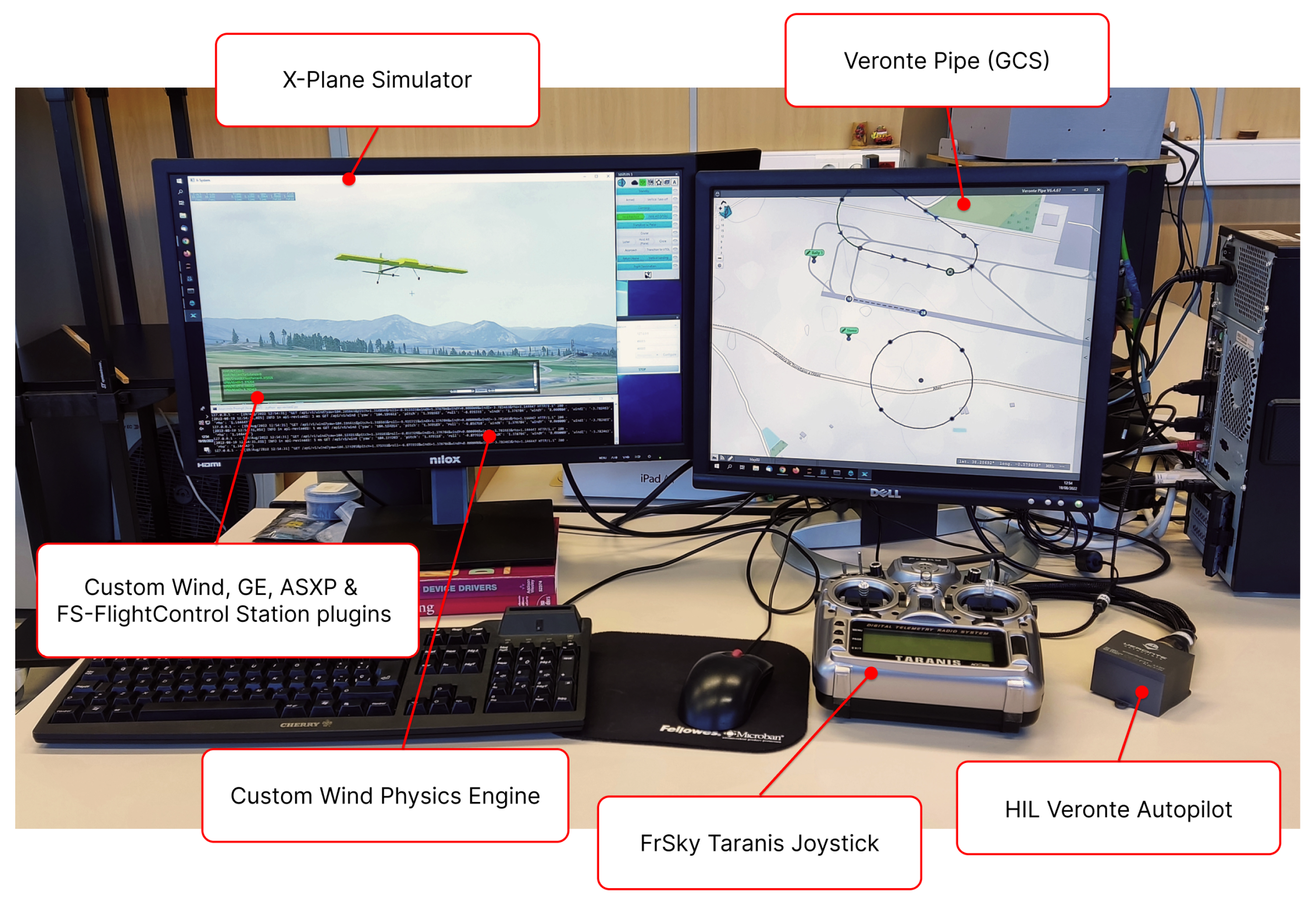
7. Materials and Methods

The whole VTOL UAV Simulator System layout is summarized in Figure 6. The simulator is subdivided into three subsystems that can be run independently when connected to X-Plane:

• Weather and Physics simulator: including the Active Sky XP plugin, our custom wind physics engine and X-Plane plugin, and our custom ground effect plugin.
• Flight Control HIL: including the ground control station software and the Veronte Autopilot.
• Additional plugins, such as the Instructor Operation Station.

The resulting flight simulation setup can be seen in Figure 7. The pilot is given a computer connected to two screens, a transmitter, and peripherals to control the Veronte Pipe software.

On the left screen, the pilot is presented with an instance of X-Plane running the VTOL UAV model. The right screen contains the Veronte Pipe ground control station software, where the pilot can setup a mission, load it into the UAV, and track the flight, similar to a real scenario.

A third screen outside the pilot view is used by an instructor to run the FS-FlightControl Instructor Station, to simulate failures, pause and resume the simulator when needed, and review the pilot’s performance.

This setup is currently in use by the actual VTOL UAV operators to validate mission plans, practice before flight, and basic simulator training. In the upcoming future, the authors will focus their efforts on verifying whether this simulator can provide competence development with pedagogical and economic advantages over conventional outdoors training.

An example flight comparison of our novel Weather and Physics simulator with the X-Plane internal weather physics engine can be seen in the Supplementary Video S1.

For evaluation, a flight was simulated using real conditions both with the Weather and Physics sim enabled and disabled. The local airport of Pamplona (LEPP) was selected due to its proximity to the university, access to local weather reports, and availability in X-Plane. The tests were conducted on 28 November 2022 at 10:00 UTC time, where the local conditions (as stated from METAR) were as follows:

• Wind speed: 5 knots.
• Wind direction: Variable from 270 to 030 degrees.
• Temperature: 8 degrees Celsius.
• Mean air density: 1.201 kg/m${}^3$.
• Take-off coordinates: 42${}^{\circ }$46${}^{\prime }$45${}^{″}$ N, 1${}^{\circ }$39${}^{\prime }$10${}^{″}$ W.
• Initial yaw: 250${}^{\circ }$. The aircraft nose is facing southwest.

8. Results and Discussion

The ground effect is evaluated during take-off and landing maneuvers. The result comparison is shown in Figure 8. During take-off, the total amount of force required to reach the same height above ground level (AGL) is smaller with the ground effect enabled. Note that the initial propeller force is not zero because the motors are spinning with the aircraft armed. As the aircraft gains altitude and is further from the ground, the amount of ground effect force is reduced, reaching a point where the effect is negligible, as predicted from Equation (10).

During landing, the aircraft descends so quickly that there is no visible difference in the captured graphs. Despite this, the amount of force induced by the ground effect is maximum when the propellers are closer to the ground but still producing a decent amount of vertical thrust.

Figure 9 shows the wind values in a local reference frame and the forces and moments induced by this wind in an aircraft fixed reference frame. The local coordinate system used in the figures is:

• The X axis is aligned east–west with positive X meaning east.
• The Y axis is aligned straight up and down with positive Y pointing down.
• The Z axis is aligned north–south with positive Z pointing north.

From the second graph, the wind is generating a backward drafting axial force, the sideforce is pushing the aircraft towards its left, and the normal force produces positive lift. The third graph features the aerodynamic moments induced by the wind. The L moment tries to roll the aircraft to its left, the M moment pitches the nose down, and the N moment induces a right yaw towards the incoming wind. All wind-induced forces and moments are coherent with the aircraft attitude and wind direction. Note that the slight variations in wind speed components are artificially generated by ASXP’s internal turbulence model.

Lastly, Figure 10 includes a comparison of the pitch and roll angles during a short take-off, hovering and landing with the weather and physics engine enabled and disabled. In the graph above, the aircraft height AGL is showcased for reference. As expected, when the weather and physics engine is disabled, both pitch and roll angles stay close to zero, with slight oscillations possibly due to imperfections in the flight controller tune. In contrast, when the weather and physics engine is enabled, the aircraft needs to pitch its nose down and roll at around 2 degrees to the right to maintain a stationary hover position. This is expected when an aircraft is exposed to an incoming wind from the front-right direction.

Overall, the abovementioned figures show the importance of including a wind model in flight simulation. As stated, even at low wind speeds, the pilot must take into account the wind as an additional disturbance factor, and continuously provide corrections to maintain the desired flight path or aircraft position.

9. Conclusions

Throughout this paper, a flight simulator was proposed and successfully developed for VTOL UAV pilot training of the Marvin commercial aircraft based on X-Plane. Custom plugins and a custom physics model were implemented to tackle complex scenarios such as take-off, landing, and hovering flight in the presence of wind and ground proximity.

Although these custom plugins and physics engine are designed for general use, an aerodynamic model of this particular aircraft was constructed from multiple CFD simulations. A procedure was described to adapt the simulator to any other VTOL UAV.

The effect of the implemented weather and physics engine was shown in take-off, hovering, and landing maneuvers in a simulated real case scenario demonstrating the importance of simulating wind effects in VTOL aircraft.

A commercial flight controller was employed to provide realistic flight control (HIL simulation) in a simulated environment. The result is a potentially high technological readiness level (TRL) [52] flight simulation environment for VTOL UAV pilot training of the Marvin aircraft.

References

1. Ko, A.; Ohanian, O.; Gelhausen, P. Ducted fan UAV modeling and simulation in preliminary design. In Proceedings of the AIAA Modeling and Simulation Technologies Conference and Exhibit, Hilton Head, SC, USA, 20–23 August 2007; p. 6375. [Google Scholar]
2. Tekinalp, O.; Unlu, T.; Yavrucuk, I. Simulation and flight control of a tilt duct uav. In Proceedings of the AIAA Modeling and Simulation Technologies Conference, Chicago, IL, USA, 10–13 August 2009; p. 6138. [Google Scholar]
3. Cao, J.; Anvar, A.M. Design, modelling and simulation of maritime uav-vtol flight dynamics. In Applied Mechanics and Materials; Trans Tech Publications: Cham, Switzerland, 2012; Volume 152, pp. 1533–1538. [Google Scholar]
4. Muraoka, K.; Okada, N.; Kubo, D.; Sato, M. Transition flight of quad tilt wing VTOL UAV. In Proceedings of the 28th Congress of the International Council of the Aeronautical Sciences, Brisbane, Australia, 23–28 September 2012. [Google Scholar]
5. Ke, Y.; Chen, B.M. Full envelope dynamics modeling and simulation for tail-sitter hybrid UAVs. In Proceedings of the 2017 36th Chinese Control Conference (CCC), Dalian, China, 26–28 July 2017; pp. 2242–2247. [Google Scholar] [CrossRef]
6. Lyu, X.; Gu, H.; Zhou, J.; Li, Z.; Shen, S.; Zhang, F. Simulation and flight experiments of a quadrotor tail-sitter vertical take-off and landing unmanned aerial vehicle with wide flight envelope. Int. J. Micro Air Veh. 2018, 10, 303–317. [Google Scholar] [CrossRef] [Green Version]
7. Walid, M.; Slaheddine, N.; Mohamed, A.; Lamjed, B. Modeling and control of a quadrotor UAV. In Proceedings of the 2014 15th International Conference on Sciences and Techniques of Automatic Control and Computer Engineering (STA), Hammamet, Tunisia, 21–23 December 2014; pp. 343–348. [Google Scholar] [CrossRef]
8. Lyu, X.; Gu, H.; Wang, Y.; Li, Z.; Shen, S.; Zhang, F. Design and implementation of a quadrotor tail-sitter VTOL UAV. In Proceedings of the 2017 IEEE International Conference on Robotics and Automation (ICRA), Singapore, 29 May–3 June 2017; pp. 3924–3930. [Google Scholar] [CrossRef]
9. Oosedo, A.; Konno, A.; Matsumoto, T.; Go, K.; Masuko, K.; Uchiyama, M. Design and attitude control of a quad-rotor tail-sitter vertical takeoff and landing unmanned aerial vehicle. Adv. Robot. 2012, 26, 307–326. [Google Scholar] [CrossRef]
10. Carlson, S.J.; Papachristos, C. The MiniHawk-VTOL: Design, Modeling, and Experiments of a Rapidly-prototyped Tiltrotor UAV. In Proceedings of the 2021 International Conference on Unmanned Aircraft Systems (ICUAS), Athens, Greece, 15–18 June 2021; pp. 777–786. [Google Scholar] [CrossRef]
11. ERSOY, E.; YALÇIN, M.K. Designing autopilot system for fixed-wing flight mode of a tilt-rotor UAV in a virtual environment: X-Plane. Int. Adv. Res. Eng. J. 2018, 2, 33–42. [Google Scholar]
12. Yu, L.; He, G.; Zhao, S.; Wang, X.; Shen, L. Design and implementation of a hardware-in-the-loop simulation system for a tilt trirotor UAV. J. Adv. Transp. 2020, 2020, 4305742. [Google Scholar] [CrossRef]
13. D’Urso, F.; Santoro, C.; Santoro, F.F. Integrating Heterogeneous Tools for Physical Simulation of multi-Unmanned Aerial Vehicles. In Proceedings of the WOA, Palermo, Italy, 28–29 June 2018; pp. 10–15. [Google Scholar]
14. Vuruskan, A.; Yuksek, B.; Ozdemir, U.; Yukselen, A.; Inalhan, G. Dynamic modeling of a fixed-wing VTOL UAV. In Proceedings of the 2014 International Conference on Unmanned Aircraft Systems (ICUAS), Orlando, FL, USA, 27–30 May 2014; pp. 483–491. [Google Scholar] [CrossRef]
15. Caro, P.W. Aircraft simulators and pilot training. Hum. Factors 1973, 15, 502–509. [Google Scholar] [CrossRef]
16. McLean, G.M.; Lambeth, S.; Mavin, T. The use of simulation in ab initio pilot training. Int. J. Aviat. Psychol. 2016, 26, 36–45. [Google Scholar] [CrossRef]
17. Gu, H.; Wu, D.; Liu, H. Development of a novel low-cost flight simulator for pilot training. Int. J. Comput. Syst. Eng. 2009, 3, 1581–1585. [Google Scholar]
18. Dahlstrom, N.; Dekker, S.; van Winsen, R.; Nyce, J. Fidelity and validity of simulator training. In Simulation in Aviation Training; Routledge: London, UK, 2017; pp. 135–144. [Google Scholar]
19. Craighead, J.; Murphy, R.; Burke, J.; Goldiez, B. A Survey of Commercial & Open Source Unmanned Vehicle Simulators. In Proceedings of the 2007 IEEE International Conference on Robotics and Automation, Roma, Italy, 10–14 April 2007; pp. 852–857. [Google Scholar] [CrossRef]
20. Bittar, A.; Figuereido, H.V.; Guimaraes, P.A.; Mendes, A.C. Guidance Software-In-the-Loop simulation using X-Plane and Simulink for UAVs. In Proceedings of the 2014 International Conference on Unmanned Aircraft Systems (ICUAS), Orlando, FL, USA, 27–30 May 2014; pp. 993–1002. [Google Scholar] [CrossRef]
21. Nguyen, K.D.; Ha, C.; Jang, J.T. Development of a new hybrid drone and software-in-the-loop simulation using px4 code. In Proceedings of the International Conference on Intelligent Computing, Wuhan, China, 15–18 August 2018; Springer: Cham, Switzerland, 2018; pp. 84–93. [Google Scholar]
22. Ganoni, O.; Mukundan, R. A framework for visually realistic multi-robot simulation in natural environment. arXiv 2017, arXiv:1708.01938. [Google Scholar]
23. Soltani, A.; Assadian, F. A Hardware-in-the-Loop Facility for Integrated Vehicle Dynamics Control System Design and Validation. In Proceedings of the 7th IFAC Symposium on Mechatronic Systems MECHATRONICS 2016, Loughborough, UK, 5–8 September 2016; IFAC-PapersOnLine. Volume 49, pp. 32–38. [Google Scholar] [CrossRef]
24. Nicolescu, G.; Mosterman, P.J. Model-Based Design for Embedded Systems; CRC Press: Boca Raton, FL, USA, 2018. [Google Scholar]
25. Gausemeier, J.; Moehringer, S. VDI 2206- A New Guideline for the Design of Mechatronic Systems. In Proceedings of the 2nd IFAC Conference on Mechatronic Systems, Berkeley, CA, USA, 9–11 December 2022; IFAC Proceedings Volumes. Volume 35, pp. 785–790. [Google Scholar] [CrossRef]
26. MathWorks. Validation and Verification for System Development. 2022. Available online: https://mathworks.com/help/rtw/gs/v-model-for-system-development.html (accessed on 15 November 2022).
27. Sun, J.; Li, B.; Wen, C.Y.; Chen, C.K. Design and implementation of a real-time hardware-in-the-loop testing platform for a dual-rotor tail-sitter unmanned aerial vehicle. Mechatronics 2018, 56, 1–15. [Google Scholar] [CrossRef]
28. Garcia-Nieto, S.; Velasco-Carrau, J.; Paredes-Valles, F.; Salcedo, J.V.; Simarro, R. Motion equations and attitude control in the vertical flight of a VTOL bi-rotor UAV. Electronics 2019, 8, 208. [Google Scholar] [CrossRef] [Green Version]
29. Astuti, G.; Longo, D.; Melita, C.; Muscato, G.; Orlando, A. HIL tuning of UAV for exploration of risky environments. Int. J. Adv. Robot. Syst. 2008, 5, 36. [Google Scholar] [CrossRef]
30. Adiprawita, W.; Ahmad, A.S.; Semibiring, J. Hardware in the loop simulator in UAV rapid development life cycle. arXiv 2008, arXiv:0804.3874. [Google Scholar]
31. Yoo, C.s.; Kang, Y.s.; Park, B.j. Hardware-In-the-Loop simulation test for actuator control system of Smart UAV. In Proceedings of the ICCAS 2010, Gyeonggi-do, Republic of Korea, 27–30 October 2010; pp. 1729–1732. [Google Scholar] [CrossRef]
32. Drela, M. XFOIL: An analysis and design system for low Reynolds number airfoils. In Low Reynolds Number Aerodynamics; Springer: Berlin/Heidelberg, Germany, 1989; pp. 1–12. [Google Scholar]
33. Tsien, H.S.; Lees, L. The Glauert-Prandtl approximation for subsonic flows of a compressible fluid. J. Aeronaut. Sci. 1945, 12, 173–187. [Google Scholar] [CrossRef]
34. Selig, M.S. Real-time flight simulation of highly maneuverable unmanned aerial vehicles. J. Aircr. 2014, 51, 1705–1725. [Google Scholar] [CrossRef]
35. Isermann, R.; Schaffnit, J.; Sinsel, S. Hardware-in-the-loop simulation for the design and testing of engine-control systems. Control. Eng. Pract. 1999, 7, 643–653. [Google Scholar] [CrossRef]
36. Cole, J.S., Jr.; Jolly, A.C. Hardware-in-the-loop simulation at the US Army Missile Command. In Proceedings of the Technologies for Synthetic Environments: Hardware-in-the-Loop Testing, Orlando, FL, USA, 8–12 April 1996; Volume 2741, pp. 14–19. [Google Scholar]
37. Sisle, M.E.; McCarthy, E.D. Hardware-in-the-loop simulation for an active missile. Simulation 1982, 39, 159–167. [Google Scholar] [CrossRef]
38. Eguchi, H.; Yamashita, T. Benefits of HWIL simulation to develop guidance and control systems for missiles. In Proceedings of the Technologies for Synthetic Environments: Hardware-in-the-Loop Testing V, Orlando, FL, USA, 24–28 April 2000; Volume 4027, pp. 66–73. [Google Scholar]
39. Autopiloto para Drone Veronte 1x–UAV Autopilots–Productos Veronte. 2022. Available online: https://www.embention.com/es/producto/autopiloto-simple/ (accessed on 20 September 2022).
40. Aláez, D.; Olaz, X.; Prieto, M.; Villadangos, J.; Astrain, J. VTOL UAV digital twin for take-off, hovering and landing in different wind conditions. Simul. Model. Pract. Theory 2022, 102703. [Google Scholar] [CrossRef]
41. Grinberg, M. Flask Web Development: Developing Web Applications with Python; O’Reilly Media, Inc.: Newton, MA, USA, 2018. [Google Scholar]
42. D’Urso, F.; Santoro, C.; Santoro, F.F. Wale: A solution to share libraries in Docker containers. Future Gener. Comput. Syst. 2019, 100, 513–522. [Google Scholar] [CrossRef]
43. Active Sky XP Home Page. Available online: https://hifisimtech.com/asxp/ (accessed on 14 September 2022).
44. Aich, S.; Ahuja, C.; Gupta, T.; Arulmozhivarman, P. Analysis of ground effect on multi-rotors. In Proceedings of the 2014 International Conference on Electronics, Communication and Computational Engineering (ICECCE), Hosur, India, 17–18 November 2014; IEEE: Piscataway, NJ, USA, 2014; pp. 236–241. [Google Scholar]
45. Betz, A. The Ground Effect on Lifting Propellers; Technical Report TM 836; National Advisory Committee for Aeronautics: Washington, DC, USA, 1937. [Google Scholar]
46. Knight, M.; Hegner, R.A. Analysis of Ground Effect on the Lifting Airscrew; Technical Report TN 835; National Advisory Committee for Aeronautics: Washington, DC, USA, 1941. [Google Scholar]
47. Zbrozek, J. Ground Effect on the Lifting Rotor; Technical Report RM 2347; Aeronautical Research Council: London, UK, 1947. [Google Scholar]
48. Cheeseman, I.; Bennett, W. The Effect of the Ground on a Helicopter Rotor in Forward Flight; Cranfield University: Bedford, UK, 1955. [Google Scholar]
49. Fradenburgh, E.A. The helicopter and the ground effect machine. J. Am. Helicopter Soc. 1960, 5, 24–33. [Google Scholar] [CrossRef]
50. Marr, R.; Ford, D.; Ferguson, S. Analysis of the Wind Tunnel Test of a Tilt Rotor Power Force Model; Technical Report NASA-CR-137529; National Aeronautics and Space Administration: Moffett Field, CA, USA, 1974. [Google Scholar]
51. Hayden, J.S. The effect of the ground on helicopter hovering power required. In Proceedings of the AHS 32nd Annual Forum, Winnipeg, MB, Canada, 5 November 1976. [Google Scholar]
52. Conrow, E.H. Estimating technology readiness level coefficients. J. Spacecr. Rocket. 2011, 48, 146–152. [Google Scholar] [CrossRef]
Figure 1. 3D renders of the VTOL UAV both in copter mode (top) and plane (bottom) mode.
Information 13 00585 g001
Figure 2. X-Plane’s Airfoil Maker screenshot featuring manually-adjusted aerodynamic coefficient curves of an airfoil.
Information 13 00585 g002
Figure 3. X-Plane’s Plane Maker screenshot featuring the VTOL UAV model.
Information 13 00585 g003
Figure 4. Meshing tool screenshot from Ansys featuring the simplified 3D model and Ansys default axes.
Information 13 00585 g004
Figure 5. Weather and physics subsystem integration scheme. The Custom X-Plane Ground Effect Plugin was omitted from this diagram since it will be explained in the following subsection.
Information 13 00585 g005
Figure 6. VTOL UAV Simulator System block diagram featuring all three subsystems connected to X-Plane.
Information 13 00585 g006
Figure 7. Annotated photograph of the full working setup as seen by a pilot during training.
Information 13 00585 g007
Figure 8. Take−off and landing normal forces comparison with and without ground effect.
Information 13 00585 g008
Figure 9. Forces and moments induced by wind using our custom weather and physics engine.
Information 13 00585 g009
Figure 10. Short flight comparison of pitch and roll angles with and without our custom weather and physics engine.
Information 13 00585 g010