
An Efficient Malware Classification Method Based on the AIFS-IDL and Multi-Feature Fusion


Abstract
1. Introduction
- A static malware classification method that integrates multiple features is proposed. The proposed method extracts six malware features from the disassembly and byte files and integrates the advantages of different features to improve the classification accuracy;
- Feature extraction capability of TCN for temporal data is introduced to fully learn the dependency relationship among data; The nonlinear fitting ability of GRU is used after information in the sequence, extracting the malware features based on the time series to improve the model classification effect; CNN has the characteristics of simple structure and low complexity. TCN, GRU, and CNN are used to learn the information on the extracted features fully;
- The IFS and MAGDM methods are introduced to integrate the classification results and optimize the uncertainty, thus improving the classification accuracy and generalization ability of the deep learning algorithm.
2. Related Work and Technology
2.1. IFS and MAGDM
- (DP1) ;
- (DP2) ;
- (DP3) ;
- (DP4) ;
- (DP5)
- (DP1) ;
- (DP2) ;
- (DP3) ;
- (DP4) ;
- (DP5)
2.2. Deep Learning Models
- (a)
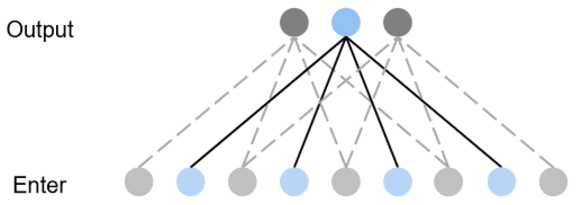
- Causal convolution: An output at time t is related only to the input at time t and the input of the previous layer [26]. Traditional CNN can see future information, whereas causal convolution can see only past information. Therefore, the causal convolution has a very strict time constraint and represents a one-way structure. A single causal convolution structure is shown in Figure 1a, and the overall structure is shown in Figure 1b, for a convolution kernel number off four. Using four convolution kernels means that four points are sampled from the previous layer as the input of the next layer;
- (b)
- Dilated Convolution: With the increase in the number of dilated convolution layers, the expansion coefficient increases exponentially, and the increase in the receptive field of a layer will reduce the number of convolution layers. This reduces the amount of calculation and simplifies the network structure. In view of the traditional neural networks problem that time-series data modeling can only be extended by linearly stacking multi-layer convolutions, TCN uses dilated convolution to increase the receptive field of a layer to reduce the number of convolutional layers [27]. The network structure for a convolution kernel number of four and an expansion coefficient of one is shown in Figure 2. When the expansion coefficient of the input layer is one, the model samples data from the previous layer with an interval of one and inputs them to the next layer.
- (c)
- Residual block: Residual block is an important part of the TCN structure. As shown in Figure 3, a residual block includes a dilated causal convolution layer and a nonlinear mapping layer and has an identity mapping method that connects layers, enabling the network to transmit information across layers. Residual connection can both increase the response and convergence speed of a deep network and solve the problem of slow learning speed caused by complex layer structure. Moreover, dropout and batch normalization are added to the residual block to prevent model overfitting and increase the training speed [28].
3. AIFS Malware Classification Based on Ensemble Deep Learning
3.1. Feature Extraction
- 1.
- Data sections
- 2.
- Data definition
- 3.
- API features
- 4.
- Entropy feature
- 5.
- Haralick features
- 6.
- String features
3.2. IFS-MAGDM
- When , ;
- When , ;
- When , .
4. Experimental Results
4.1. Experimental Setup
- Experiment 1: Single-feature comparison;
- Experiment 2: Multi-feature fusion comparison;
- Experiment 3: Comparison of different classification algorithms.
4.2. Evaluation Indices
4.3. Hardware and Dataset
4.4. Single-Feature Comparison
4.5. Multi-Feature Fusion Comparison
4.6. Comparison of Different Classification Algorithms
5. Conclusions and Future Work
Author Contributions
Funding
Data Availability Statement
Conflicts of Interest
References
- Zhao, J.; Zhang, S.; Liu, B.; Cui, B. Malware detection using machine learning based on the combination of dynamic and static features. In Proceedings of the 2018 27th International Conference on Computer Communication and Networks (ICCCN), Hangzhou, China, 30 July–2 August 2018. [Google Scholar]
- Yang, P.; Pan, Y.; Jia, P.; Liu, L. Research on malware detection based on vector features of assembly instructions. Inf. Secur. Res. 2020, 6, 113–121. [Google Scholar]
- Raff, E.; Sylvester, J.; Nicholas, C. Learning the pe header, malware detection with minimal domain knowledge. In Proceedings of the 10th ACM Workshop on Artificial Intelligence and Security, Dallas, TX, USA, 3 November 2017; pp. 121–132. [Google Scholar]
- Zhao, S.; Ma, X.; Zou, W.; Bai, B. DeepCG: Classifying metamorphic malware through deep learning of call graphs. In Proceedings of the International Conference on Security and Privacy in Communication Systems, Orlando, FL, USA, 23–25 October 2019; pp. 171–190. [Google Scholar]
- Santos, I.; Brezo, F.; Ugarte-Pedrero, X.; Bringas, P.G. Opcode sequences as representation of executables for data-mining-based unknown malware detection. Inf. Sci. 2013, 231, 64–82. [Google Scholar] [CrossRef]
- Kang, B.; Yerima, S.Y.; McLaughlin, K.; Sezer, S. N-opcode Analysis for Android Malware Classification and Categorization. In Proceedings of the 2016 International Conference on Cyber Security and Protection of Digital Services (Cyber Security), London, UK, 13–14 June 2016; pp. 1–7. [Google Scholar]
- Nataraj, L.; Karthikeyan, S.; Jacob, G.; Manjunath, B.S. Malware images: Visualization and automatic classification. In Proceedings of the VizSec ′11: Proceedings of the 8th International Symposium on Visualization for Cyber Security, Pittsburgh, PA, USA, 20 July 2011; Volume 4. [Google Scholar] [CrossRef]
- Gibert, D.; Mateu, C.; Planes, J. Orthrus: A Bimodal Learning Architecture for Malware Classification. In Proceedings of the 2020 International Joint Conference on Neural Networks (IJCNN), Glasgow, UK, 19–24 July 2020; pp. 1–8. [Google Scholar]
- Kwon, I.; Im, E.G. Extracting the Representative API Call Patterns of Malware Families Using Recurrent Neural Network. In Proceedings of the International Conference, Krakow Poland, 20–23 September 2017; pp. 202–207. [Google Scholar]
- Kolosnjaji, B.; Zarras, A.; Webster, G.; Eckert, C. Deep learning for classification of malware system call sequences. In Proceedings of the Australasian Joint Conference on Artificial Intelligence, Hobart, Australia, 5–8 December 2016; pp. 137–149. [Google Scholar]
- Atanassov, K. Intuitionistic fuzzy sets. Fuzzy Sets Syst. 1986, 20, 87–96. [Google Scholar] [CrossRef]
- Das, S.; Dutta, B.; Guha, D. Weight computation of criteria in a decision-making problem by knowledge measure with intuitionistic fuzzy set and interval-valued intuitionistic fuzzy set. Soft Comput. 2015, 20, 3421–3442. [Google Scholar] [CrossRef]
- Zadeh, L.A. Fuzzy sets. Inf. Control 1965, 8, 338–353. [Google Scholar] [CrossRef]
- Pal, N.R.; Bustince, H.; Pagola, M.; Mukherjee, U.K.; Goswami, D.P.; Beliakov, G. Uncertainties with Atanassov’s intuitionistic fuzzy sets: Fuzziness and lack of knowledge. Inf. Sci. 2013, 228, 61–74. [Google Scholar] [CrossRef]
- Nguyen, H. A new knowledge-based measure for intuitionistic fuzzy sets and its application in multiple attribute group decision making. Expert. Syst. Appl. 2015, 42, 8766–8774. [Google Scholar] [CrossRef]
- Chen, S.M.; Tan, J.M. Handling multicriteria fuzzy decision making problems based on vague set theory. Fuzzy Sets and Systems 1994, 67, 163–172. [Google Scholar] [CrossRef]
- Wu, X.; Song, Y.; Wang, Y. Distance-Based Knowledge Measure for Intuitionistic Fuzzy Sets with Its Application in Decision Making. Entropy 2021, 23, 1119. [Google Scholar] [CrossRef]
- Wu, X.; Huang, F.; Hu, Z.; Huang, H. Faster Adaptive Federated Learning. arXiv 2022, arXiv:2212.00974v1. [Google Scholar]
- Xu, Z. A survey of preference relations. Int. J. Gen. Syst. 2007, 36, 179–203. [Google Scholar] [CrossRef]
- Bustince, H.; Pagola, M.; Mesiar, R.; Hullermeier, E.; Herrera, F. Grouping, Overlap, and Generalized Bientropic Functions for Fuzzy Modeling of Pairwise Comparisons. IEEE Trans. Fuzzy Syst. 2011, 20, 405–415. [Google Scholar] [CrossRef]
- Mou, Q.; Xu, Z.; Liao, H. A graph based group decision making approach with intuitionistic fuzzy preference relations. Comput. Ind. Eng. 2017, 110, 138–150. [Google Scholar] [CrossRef]
- Xiang, Q.; Wang, X.; Song, Y.; Lei, L.; Li, R.; Lai, J. One-dimensional convolutional neural networks for high-resolution range profile recognition via adaptively feature recalibrating and automatically channel pruning. Int. J. Intell. Syst. 2021, 36, 332–361. [Google Scholar] [CrossRef]
- Xiang, Q.; Wang, X.; Lai, J.; Song, Y.; Li, R.; Lei, L. Multi-scale group-fusion convolutional neural network for high-resolution range profile target recognition. IET Radar Sonar Navig. 2022, 16, 1997–2016. [Google Scholar] [CrossRef]
- Bai, S.; Kolter, J.Z.; Koltun, V. An empirical evaluation of generic convolutional and recurrent networks for sequence modeling. arXiv 2018, arXiv:1803.01271. [Google Scholar]
- Fan, Y.Y.; Li, C.J.; Yi, Q.; Li, B.Q. Classification of Field Moving Targets Based on Improved TCN Network. Comput. Eng. 2012, 47, 106–112. [Google Scholar]
- Yating, G.; Wu, W.; Qiongbin, L.; Fenghuang, C.; Qinqin, C. Fault Diagnosis for Power Converters Based on Optimized Temporal Convolutional Network. IEEE Trans. Instrum. Meas. 2020, 70, 1–10. [Google Scholar] [CrossRef]
- Huang, Q.; Hain, T. Improving Audio Anomalies Recognition Using Temporal Convolutional Attention Network. In Proceedings of the ICASSP 2021–2021 IEEE International Conference on Acoustics, Speech and Signal Processing (ICASSP), Toronto, ON, Canada, 6–11 June 2021. [Google Scholar] [CrossRef]
- Zhu, R.; Liao, W.; Wang, Y. Short-term prediction for wind power based on temporal convolutional network. Energy Rep. 2020, 6, 424–429. [Google Scholar] [CrossRef]
- Xu, Z.; Zeng, W.; Chu, X.; Cao, P. Multi-Aircraft Trajectory Collaborative Prediction Based on Social Long Short-Term Memory Network. Aerospace 2021, 8, 115. [Google Scholar] [CrossRef]
- Liu, Y.; Ma, J.; Tao, Y.; Shi, L.; Wei, L.; Li, L. Hybrid Neural Network Text Classification Combining TCN and GRU. In Proceedings of the 2020 IEEE 23rd International Conference on Computational Science and Engineering (CSE), Guangzhou, China, 29 December 2020–1 Januray 2021; pp. 30–35. [Google Scholar]
- Sun, Y.C.; Tian, R.L.; Wang, X.F. Emitter signal recognition based on improved CLDNN. Syst. Eng. Electron. 2021, 43, 42–47. [Google Scholar]
- Digital Bread Crumbs: Seven Clues to Identifying Who’s Behind Advanced Cyber Attacks [EB/OL]. Available online: https://www.techrepublic.com/resource-library/whitepapers/digital-bread-crumbs-seven-clues-to-identifying-who-is-behind-advanced-cyber-attacks/ (accessed on 1 August 2022).
- Microsoft Malware Classification Challenge (Big 2015). 2015. Available online: https://www.kaggle.com/c/malware-classification/data (accessed on 13 April 2015).
- Lee, J.; Pak, J.; Lee, M. Network intrusion detection system using feature extraction based on deep sparse autoencoder. In Proceedings of the 2020 International Conference on Information and Communication Technology Convergence (ICTC), Jeju, Korea, 21–23 October 2020. [Google Scholar]
- Injadat, M.N.; Moubayed, A.; Nassif, A.B.; Shami, A. Multi-Stage Optimized Machine Learning Framework for Network Intrusion Detection. IEEE Trans. Netw. Serv. Manag. 2020, 18, 1803–1816. [Google Scholar] [CrossRef]
- Di Mauro, M.; Galatro, G.; Fortino, G.; Liotta, A. Supervised feature selection techniques in network intrusion detection: A critical review. Eng. Appl. Artif. Intell. 2021, 101, 104216. [Google Scholar] [CrossRef]
- Yan, J.; Qi, Y.; Rao, Q. Detecting Malware with an Ensemble Method Based on Deep Neural Network. Secur. Commun. Netw. 2018, 2018, 7247095. [Google Scholar] [CrossRef]
- Burnaev, E.; Smolyakov, D. One-Class SVM with Privileged Information and Its Application to Malware Detection. In Proceedings of the 2016 IEEE 16th International Conference on Data Mining Workshops (ICDMW), Barcelona, Spain, 12–15 December 2016; pp. 273–280. [Google Scholar] [CrossRef]
- Narayanan, B.N.; Djaneye-Boundjou, O.; Kebede, T.M. Performance analysis of machine learning and pattern recognition algorithms for Malware classification. In Proceedings of the 2016 IEEE National Aerospace and Electronics Conference (NAECON) and Ohio Innovation Summit (OIS), Dayton, OH, USA, 25–29 July 2017; pp. 338–342. [Google Scholar] [CrossRef]
- Drew, J.; Hahsler, M.; Moore, T. Polymorphic malware detection using sequence classification methods and ensembles. EURASIP J. Inf. Secur. 2017, 2017, 2. [Google Scholar] [CrossRef]
- Ni, S.; Qian, Q.; Zhang, R. Malware identification using visualization images and deep learning. Comput. Secur. 2018, 77, 871–885. [Google Scholar] [CrossRef]
- Le, Q.; Boydell, O.; Mac Namee, B.; Scanlon, M. Deep learning at the shallow end: Malware classification for non-domain experts. Digit. Investig. 2018, 26, S118–S126. [Google Scholar] [CrossRef]
- Khan, R.U.; Zhang, X.; Kumar, R. Analysis of ResNet and GoogleNet models for malware detection. J. Comput. Virol. Hacking Tech. 2019, 15, 29–37. [Google Scholar] [CrossRef]
- Marastoni, N.; Giacobazzi, R.; Preda, M.D. Data augmentation and transfer learning to classify malware images in a deep learning context. J. Comput. Virol. Hacking Tech. 2021, 17, 279–297. [Google Scholar] [CrossRef]
- Darem, A.; Abawajy, J.; Makkar, A.; Alhashmi, A.; Alanazi, S. Visualization and deep-learning-based malware variant detection using OpCode-level features. Future Gener. Comput. Syst. 2021, 125, 314–323. [Google Scholar] [CrossRef]
- Wu, X.; Song, Y.; Hou, X.; Ma, Z.; Chen, C. Deep Learning Model with Sequential Features for Malware Classification. Appl. Sci. 2022, 12, 9994. [Google Scholar] [CrossRef]
- Di Mauro, M.; Galatro, G.; Liotta, A. Experimental review of neural-based approaches for network intrusion management. IEEE Trans. Netw. Serv. Manag. 2020, 17, 2480–2495. [Google Scholar] [CrossRef]
- Dong, S.; Xia, Y.; Peng, T. Network Abnormal Traffic Detection Model Based on Semi-Supervised Deep Reinforcement Learning. IEEE Trans. Netw. Serv. Manag. 2021, 18, 4197–4212. [Google Scholar] [CrossRef]
- Pelletier, C.; Webb, G.I.; Petitjean, F. Deep learning for the classification of Sentinel-2 image time series. In Proceedings of the IGARSS 2019-2019 IEEE International Geoscience and Remote Sensing Symposium, Yokohama, Japan, 28 July–2 August 2019. [Google Scholar]


| Name | Description |
|---|---|
| .text | Code section; program code segment identifier |
| .data | Data section; initialize data segment, store global data, and global constants |
| .bss | Uninitialized data segment; store global data and global constants |
| .rdata | Resource data segment |
| .edata | Export table; addresses of exported external functions |
| .idata | Import table; addresses of imported external functions |
| .rsrc | Resource section; store program resources such as icons and menus |
| .tls | Store pre-stored thread-local variables, including initialization data, callback functions for each thread initialization and termination, and TLS index |
| .reloc | Base address relocation table; all content in the mirror that needs to be relocated |
| Name | Description |
|---|---|
| Num_Sections | Total number of sections |
| Unknown_Sections | Number of unknown sections |
| Unknown_Sections_lines | Number of lines in unknown sections |
| known_Sections_por | Proportion of known sections |
| Unknown_Sections_por | Proportion of unknown sections |
| Unknown_Sections_lines_por | Proportion of lines in unknown sections |
| Unknown_Sections_lines_por | Proportion of lines in unknown sections |
| Name | Description |
|---|---|
| API_GetProcAddress | Retrieves the output library function address from the specified dynamic link library (DLL). |
| API_LoadLibraryA | Loads the specified module into the address space of the calling process. The specified module may cause other modules to be loaded. |
| API_GetModuleHandleA | Retrieves a module handle for the specified module. The module must have been loaded by the calling process. |
| API_ExitProcess | Ends the calling process and all its threads. |
| API_VirtualAlloc | Reserves, commits, or changes the state of a region of pages in the virtual address space of the calling process. Memory allocated by this function is automatically initialized to zero. |
| API_WriteFile | Writes data to the specified file or input/output (I/O) device. |
| Features | Model | Accuracy | Precision | Recall | F1-Score | |
|---|---|---|---|---|---|---|
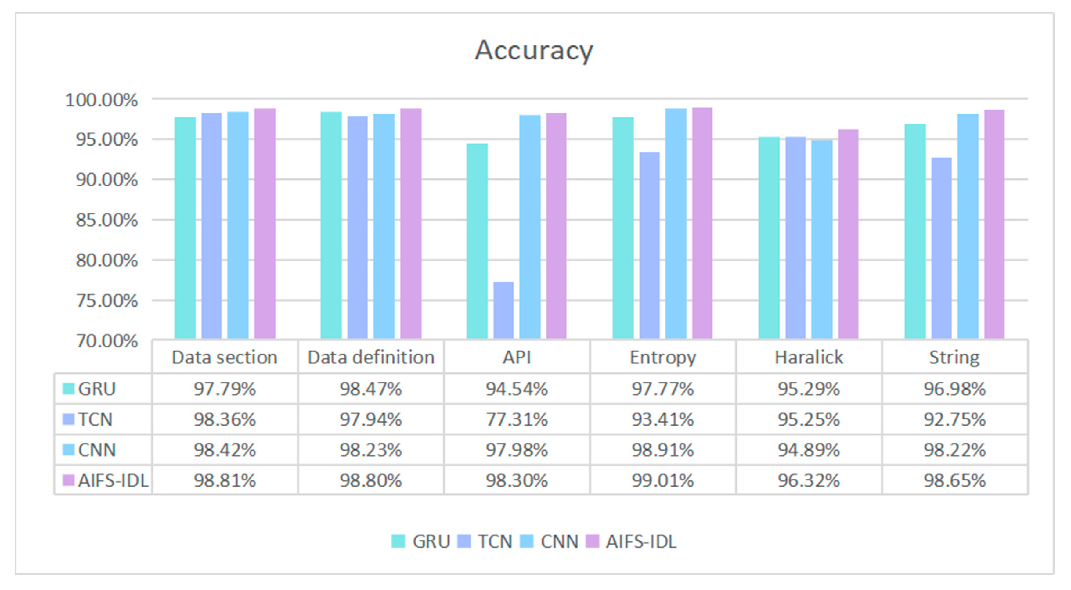
| Features from the .asm file | Data section | GRU | 97.79% | 97.34% | 97.41% | 97.35% |
| TCN | 98.36% | 97.81% | 97.72% | 97.72% | ||
| CNN | 98.42% | 98.24% | 98.16% | 98.18% | ||
| AIFS-IDL | 98.81% | 98.62% | 98.52% | 98.50% | ||
| Data definition | GRU | 98.47% | 97.49% | 97.50% | 97.48% | |
| TCN | 97.94% | 97.62% | 97.57% | 97.58% | ||
| CNN | 98.23% | 97.91% | 97.90% | 97.91% | ||
| AIFS-IDL | 98.50% | 98.53% | 98.52% | 98.64% | ||
| API | GRU | 94.54% | 94.18% | 94.02% | 94.02% | |
| TCN | 77.31% | 80.49% | 76.45% | 74.54% | ||
| CNN | 97.98% | 97.74% | 97.55% | 97.57% | ||
| AIFS-IDL | 98.30% | 98.25% | 98.17% | 98.22% | ||
| Features from the byte file | Entropy | GRU | 97.77% | 97.09% | 97.20% | 97.13% |
| TCN | 93.41% | 92.38% | 92.38% | 92.18% | ||
| CNN | 98.91% | 98.50% | 98.60% | 98.54% | ||
| AIFS-IDL | 99.01% | 98.56% | 98.67% | 98.56% | ||
| Haralick | GRU | 95.29% | 94.21% | 94.33% | 94.23% | |
| TCN | 95.25% | 94.23% | 94.33% | 94.24% | ||
| CNN | 94.89% | 94.34% | 94.42% | 94.31% | ||
| AIFS-IDL | 95.32% | 94.65% | 94.76% | 94.28% | ||
| String | GRU | 96.98% | 96.97% | 96.98% | 96.94% | |
| TCN | 92.75% | 92.84% | 92.75% | 92.59% | ||
| CNN | 98.22% | 97.81% | 97.89% | 97.85% | ||
| AIFS-IDL | 98.35% | 98.03% | 98.06% | 97.97% | ||
| Features | Model | Accuracy | Precision | Recall | F1-Score |
|---|---|---|---|---|---|
| Features from the .asm file | GRU | 99.63% | 99.64% | 99.63% | 99.62% |
| TCN | 99.36% | 99.36% | 99.36% | 99.36% | |
| CNN | 99.36% | 99.00% | 98.99% | 98.97% | |
| AIFS-IDL | 99.84% | 99.86% | 99.85% | 99.85% | |
| Features from the .byte file | GRU | 99.26% | 99.27% | 99.26% | 99.25% |
| TCN | 98.07% | 97.91% | 98.07% | 97.98% | |
| CNN | 98.99% | 98.91% | 98.90% | 98.88% | |
| AIFS-IDL | 99.46% | 99.47% | 99.46% | 99.45% | |
| All features | GRU | 99.72% | 99.73% | 99.72% | 99.73% |
| TCN | 99.45% | 99.46% | 99.45% | 99.46% | |
| CNN | 99.45% | 99.37% | 99.36% | 99.34% | |
| AIFS-IDL | 99.92% | 99.92% | 99.92% | 99.92% |
| Authors | Time | Method | Model | Features | Accuracy |
|---|---|---|---|---|---|
| Burnaev et al. [38] | 2016 | One-class SVM | SVM | Opcode + grayscale image | 92% |
| Narayanan et al. [39] | 2016 | PCA and kNN | KNN | grayscale image | 96.6% |
| Drew et al. [40] | 2017 | Strand Gene Sequence | Strand | asm sequence | 98.59% |
| Ni et al. [41] | 2018 | Sim–Hash and NN | CNN | Grayscale images | 98.86% |
| Le et al. [42] | 2018 | - | CNN, LSTM and RNN | Binary representation | 98.20% |
| Yan et al. [37] | 2018 | MalNet | CNN and LSTM | Raw file data | 99.36% |
| Khan et al. [43] | 2019 | - | ResNet and GoogleNet | Image | 88.36% |
| Gibert et al. [8] | 2020 | Orthrus | CNN | Byte + Opcode | 99.24% |
| Marastoni et al. [44] | 2021 | - | CNN and LSTM | Image-based data | 98.5% |
| Darem et al. [45] | 2021 | ensemble | CNN and XGBoost | Opcode + image+ segment + other | 99.12% |
| X et al. [46] | 2022 | TCN-BiGRU | TCN and BiGRU | Opcode + Byte sequence | 99.72% |
| AIFS-IDL | current | AIFS-IDL | TCN, CNN, and GRU | Disassembly file + Byte file | 99.92% |
Publisher’s Note: MDPI stays neutral with regard to jurisdictional claims in published maps and institutional affiliations. |
© 2022 by the authors. Licensee MDPI, Basel, Switzerland. This article is an open access article distributed under the terms and conditions of the Creative Commons Attribution (CC BY) license (https://creativecommons.org/licenses/by/4.0/).
Share and Cite
Wu, X.; Song, Y. An Efficient Malware Classification Method Based on the AIFS-IDL and Multi-Feature Fusion. Information 2022, 13, 571. https://doi.org/10.3390/info13120571
Wu X, Song Y. An Efficient Malware Classification Method Based on the AIFS-IDL and Multi-Feature Fusion. Information. 2022; 13(12):571. https://doi.org/10.3390/info13120571
Chicago/Turabian StyleWu, Xuan, and Yafei Song. 2022. "An Efficient Malware Classification Method Based on the AIFS-IDL and Multi-Feature Fusion" Information 13, no. 12: 571. https://doi.org/10.3390/info13120571
APA StyleWu, X., & Song, Y. (2022). An Efficient Malware Classification Method Based on the AIFS-IDL and Multi-Feature Fusion. Information, 13(12), 571. https://doi.org/10.3390/info13120571