

Using Crypto-Asset Pricing Methods to Build Technical Oscillators for Short-Term Bitcoin Trading


Abstract
1. Introduction
2. Literature Review
2.1. Cost Analysis
2.2. Crypto-Coin Valuation
2.3. Social Network Analysis for Crypto-Asset Modeling
2.4. Active Addresses and Metcalfe’s Law
2.5. Ratios of Crypto Coins
3. Materials and Methods
3.1. Network-Value–Transaction Ratio (NVT)
3.2. Network-Value–Realized-Value Ratio (NVRV)
3.3. Network-Value–Hashrate Ratio (NVHR)
3.4. Active Addresses Metrics
3.4.1. Network-Value–Metcalfe’s Law Ratio
3.4.2. Network-Value–Odlyzko’s Law Ratio
3.5. A Variant of the INET Model for Short-Term Trading
3.6. Volt Valuation Model
3.7. Trading Strategy
3.7.1. Parameters of the Moving Averages and Z-Scores
3.7.2. Trading Strategy Evaluation Metrics
4. Results
4.1. Data
4.2. Trading Performance of Each Model
5. Robustness Checks
5.1. Trading Performances in Different Time Samples
5.2. Trading Performances with Different Thresholds
6. Discussion and Conclusions
Author Contributions
Funding
Data Availability Statement
Conflicts of Interest
Appendix A. Data Sources
- (1)
- Price data: this is free data; the source is as follows:https://studio.glassnode.com/metrics?a=BTC&category=&m=market.PriceUsdClose, accessed on 1 July 2022.
- (2)
- Network value: this is free data; the source is as follows:https://studio.glassnode.com/metrics?a=BTC&category=&m=market.MarketcapUsd, accessed on 1 July 2022.
- (3)
- Realized value: this is not free data; the source is as follows:https://studio.glassnode.com/metrics?a=BTC&category=&m=market.MarketcapRealizedUsd, accessed on 1 July 2022.
- (4)
- Active addresses: this is free data; the source is as follows:https://studio.glassnode.com/metrics?a=BTC&category=&m=addresses.ActiveCount, accessed on 1 July 2022.
- (5)
- Network hashrate: this is free data; the source is as follows:https://studio.glassnode.com/metrics?a=BTC&category=&m=mining.HashRateMean, accessed on 1 July 2022.
- (6)
- Transaction in exchange: this is not free data; the source is as follows:https://studio.glassnode.com/metrics?a=BTC&category=&m=transactions.TransfersVolumeWithinExchangesSum, accessed on 1 July 2022.
- (7)
- Risk-free rate: this is free data; the source is as follows:https://fred.stlouisfed.org/series/GS10, accessed on 1 July 2022.
Appendix B. Trading Strategies Performances


References
- Burniske, C.; Tatar, J. Cryptoassets: The Innovative Investor’s Guide to Bitcoin and Beyond; McGraw-Hill: New York, NY, USA, 2018. [Google Scholar]
- Fantazzini, D. Quantitative Finance with R and Cryptocurrencies; Amazon KDP: Seattle, WA, USA, 2019; ISBN 13-978-1090685315. [Google Scholar]
- Goutte, S.; Khaled, G.; Saadi, S. Cryptofinance: A New Currency for A New Economy; World Scientific: Singapore, 2022. [Google Scholar]
- Nakano, M.; Takahashi, A.; Takahashi, S. Bitcoin technical trading with artificial neural network. Phys. A Stat. Mech. Appl. 2018, 510, 587–609. [Google Scholar] [CrossRef]
- Huang, J.Z.; Huang, W.; Ni, J. Predicting bitcoin returns using high-dimensional technical indicators. J. Financ. Data Sci. 2019, 5, 140–155. [Google Scholar] [CrossRef]
- Gradojevic, N.; Kukolj, D.; Adcock, R.; Djakovic, V. Forecasting Bitcoin with technical analysis: A not-so-random forest? Int. J. Forecast. 2021, in press. [CrossRef]
- Ortu, M.; Uras, N.; Conversano, C.; Bartolucci, S.; Destefanis, G. On technical trading and social media indicators for cryptocurrency price classification through deep learning. Expert Syst. Appl. 2022, 198, 116804. [Google Scholar] [CrossRef]
- Woo, W. Bitcoin NVT Signal. 2018. Available online: http://charts.woobull.com/bitcoin-nvt-signal (accessed on 1 July 2022).
- Kalichkin, D. Rethinking Network Value to Transactions (NVT) Ratio. 2018. Available online: https://medium.com/cryptolab/https-medium-com-kalichkin-rethinking-nvt-ratio-2cf810df0ab0 (accessed on 1 July 2022).
- Fantazzini, D.; Zimin, S. A multivariate approach for the simultaneous modelling of market risk and credit risk for cryptocurrencies. J. Ind. Bus. Econ. 2020, 47, 19–69. [Google Scholar] [CrossRef]
- Fantazzini, D.; Calabrese, R. Crypto Exchanges and Credit Risk: Modeling and Forecasting the Probability of Closure. J. Risk Financ. Manag. 2021, 14, 516. [Google Scholar] [CrossRef]
- Fantazzini, D. Crypto-Coins and Credit Risk: Modelling and Forecasting Their Probability of Death. J. Risk Financ. Manag. 2022, 15, 304. [Google Scholar] [CrossRef]
- Berengueres, J. Valuation of Cryptocurrency Mining Operations. LEDGER 2018, 3, 60–67. [Google Scholar] [CrossRef]
- Thum, M. The economic cost of bitcoin mining. CESifo Forum 2018, 19, 43–45. [Google Scholar]
- Delgado-Mohatar, O.; Felis-Rota, M.; Fernández-Herraiz, C. The Bitcoin mining breakdown: Is mining still profitable? Econ. Lett. 2019, 184, 108492. [Google Scholar] [CrossRef]
- Benetton, M.; Compiani, G.; Morse, A. Cryptomining: Energy Use and Local Impact; University of California: Berkeley, CA, USA, 2019; working paper. [Google Scholar]
- Romanchenko, O.; Shemetkova, O.; Piatanova, V.; Kornienko, D. Approach of estimation of the fair value of assets on a cryptocurrency market. In The 2018 International Conference on Digital Science; Springer: Cham, Switzerland, 2018; pp. 245–253. [Google Scholar]
- Hargrave, J.; Sahdev, N.; Feldmeier, O. How value is created in tokenized assets. In Blockchain Economics: Implications of Distributed Ledgers-Markets, Communications Networks, and Algorithmic Reality; Melanie, S., Jason, P., Soichiro, T., Frank, W., Paolo, T., Eds.; World Scientific: Hackensack, NJ, USA, 2019; Volume 1. [Google Scholar]
- Jernej, D. Approaches to Crypto Assets Valuation. Master’s Thesis, University of Ljubljana, Ljubljana, Slovenia, 2021. [Google Scholar]
- Kaal, W.; Evans, S.; Howe, H. Digital Asset Valuation. 2022. Available online: https://ssrn.com/abstract=4033886 (accessed on 1 July 2022).
- Otte, E.; Rousseau, R. Social network analysis: A powerful strategy, also for the information sciences. J. Inf. Sci. 2002, 28, 441–453. [Google Scholar] [CrossRef]
- Wasserman, S.; Faust, K. Social Network Analysis: Methods and Applications; Cambridge University Press: Cambridge, UK, 1994. [Google Scholar]
- Yang, S.; Keller, F.B.; Zheng, L. Social Network Analysis: Methods and Examples; SAGE Publications: Thousand Oaks, CA, USA, 2016. [Google Scholar]
- Borgatti, S.P.; Everett, M.G.; Johnson, J.C. Analyzing Social Networks; SAGE publishing: Thousand Oaks, CA, USA, 2018; p. 384. [Google Scholar]
- Baumann, A.; Fabian, B.; Lischke, M. Exploring the Bitcoin Network. WEBIST 2014, 1, 369–374. [Google Scholar]
- Kondor, D.; Pósfai, M.; Csabai, I.; Vattay, G. Do the rich get richer? An empirical analysis of the Bitcoin transaction network. PLoS ONE 2014, 9, e86197. [Google Scholar]
- Liang, J.; Li, L.; Zeng, D. Evolutionary dynamics of cryptocurrency transaction networks: An empirical study. PLoS ONE 2018, 13, e0202202. [Google Scholar] [CrossRef]
- Ferretti, S.; D’Angelo, G. On the ethereum blockchain structure: A complex networks theory perspective. Concurr. Comput. Pract. Exp. 2019, 32, e5493. [Google Scholar] [CrossRef]
- Vallarano, N.; Tessone, C.J.; Squartini, T. Bitcoin Transaction Networks: An overview of recent results. Front. Phys. 2020, 8, 286. [Google Scholar] [CrossRef]
- Ao, Z.; Horvath, G.; Zhang, L. Are decentralized finance really decentralized? A social network analysis of the Aave protocol on the Ethereum blockchain. arXiv 2022, arXiv:2206.08401. [Google Scholar]
- Bonifazi, G.; Corradini, E.; Ursino, D.; Virgili, L. Defining user spectra to classify Ethereum users based on their behavior. J. Big Data 2022, 9, 1–39. [Google Scholar] [CrossRef]
- Chang, T.H.; Svetinovic, D. Data analysis of digital currency networks: Namecoin case study. In Proceedings of the 21st International Conference on Engineering of Complex Computer Systems (ICECCS), Dubai, United Arab Emirates, 6–8 November 2016; pp. 122–125. [Google Scholar]
- Motamed, A.P.; Bahrak, B. Quantitative analysis of cryptocurrencies transaction graph. Appl. Netw. Sci. 2019, 4, 1–21. [Google Scholar] [CrossRef]
- Bovet, A.; Campajola, C.; Mottes, F.; Restocchi, V.; Vallarano, N.; Squartini, T.; Tessone, C.J. The evolving liaisons between the transaction networks of Bitcoin and its price dynamics. arXiv 2019, arXiv:1907.03577. [Google Scholar]
- Li, Y.; Islambekov, U.; Akcora, C.; Smirnova, E.; Gel, Y.R.; Kantarcioglu, M. Dissecting Ethereum Blockchain Analytics: What We Learn from Topology and Geometry of the Ethereum Graph? In Proceedings of the 2020 SIAM International Conference on Data Mining, Hilton Cincinnati, OH, USA, 7–9 May 2020; pp. 523–531. [Google Scholar]
- Bonifazi, G.; Corradini, E.; Ursino, D.; Virgili, L. A Social Network Analysis–Based Approach to Investigate User Behaviour during a Cryptocurrency Speculative Bubble. J. Inf. Sci. 2021, 01655515211047428. [Google Scholar] [CrossRef]
- Alabi, K. Digital blockchain networks appear to be following Metcalfe’s Law. Electron. Commer. Res. Appl. 2017, 24, 23–29. [Google Scholar] [CrossRef]
- Peterson, T. Metcalfe’s Law as a Model for Bitcoin’s Value. Altern. Invest. Anlst. Rev. 2018, 2, 9–18. [Google Scholar] [CrossRef]
- Garcia-Monleón, F.; Danvila-del-Valle, I.; Lara, F. Intrinsic value in crypto currencies. Technol. Forecast. Soc. Chang. 2021, 162, 120393. [Google Scholar] [CrossRef]
- Stylianou, K.; Spiegelberg, L.; Herlihy, M.; Carter, N. Cryptocurrency Competition and Market Concentration in the Presence of Network Effects. LEDGER 2021, 6, 81–101. [Google Scholar] [CrossRef]
- Sabalionis, A.; Wenbo, W.; Park, H. What affects the price movements in Bitcoin and Ethereum? Manch. Sch. 2021, 89, 102–127. [Google Scholar] [CrossRef]
- Papadamou, S.; Kyriazis, N.A.; Tzeremes, P.; Corbet, S. Herding behaviour and price convergence clubs in cryptocurrencies during bull and bear markets. J. Behav. Exp. Financ. 2021, 30, 100469. [Google Scholar] [CrossRef]
- Papadamou, S.; Kyriazis, N.A.; Tzeremes, P. Non-linear causal linkages of EPU and gold with major cryptocurrencies during bull and bear markets. N. Am. J. Econ. Financ. 2021, 56, 101343. [Google Scholar] [CrossRef]
- Kyriazis, N.; Papadamou, S.; Tzeremes, P.; Corbet, S. The differential influence of social media sentiment on cryptocurrency returns and volatility during COVID-19. Q. Rev. Econ. Financ. 2022; in press. [Google Scholar] [CrossRef]
- Woo, W. Is Bitcoin in A Bubble? Check The NVT Ratio. 2017. Available online: https://www.forbes.com/sites/wwoo/2017/09/29/is-bitcoin-in-a-bubble-check-the-nvt-ratio/#af3a68b6a23f (accessed on 1 July 2022).
- Murad, M.; Puell, D. Bitcoin Market-Value-to-Realized-Value (MVRV) Ratio. Available online: ttps://medium.com/adaptivecapital/bitcoin-market-value-to-realized-value-mvrv-ratio-3ebc914dbaee (accessed on 1 July 2022).
- Liu, Y. Cryptocurrency Valuation. 2019. Available online: https://medium.com/coinmonks/cryptocurrency-valuation-d9979074404 (accessed on 1 July 2022).
- Liu, Y.; Zhang, L. Cryptocurrency valuation: An explainable AI approach. arXiv 2022, arXiv:2201.12893. [Google Scholar]
- Coinmetrics. Introducing Realized Capitalization. 2018. Available online: https://coinmetrics.io/realized-capitalization (accessed on 1 July 2022).
- Wonder, A. Introducing The Bitcoin “MVRV Z” Metric That Predicts Market Tops with 90%+ Accuracy. 2018. Available online: https://medium.com/@Awe_andWonder/introducing-the-bitcoin-mvrv-z-score-metric-that-predicts-market-tops-with-90-accuracy-89d90df043d7 (accessed on 1 July 2022).
- 21Shares. Valuing Bitcoin. 2020. Available online: https://21shares.com/research/valuing-bitcoin/ (accessed on 1 July 2022).
- Shapiro, C.; Varian, H. Information rules: A Strategic Guide to the Network Economy; Harvard Business Press: Boston, MA, USA, 1998. [Google Scholar]
- Metcalfe, B. Metcalfe’s law after 40 years of Ethernet. Computer 2013, 46, 26–31. [Google Scholar] [CrossRef]
- Odlyzko, A.; Briscoe, B.; Tilly, B. Metcalfe’s law is wrong-communications networks increase in value as they add members-but by how much? IEEE Spectr. 2006, 43, 34–39. [Google Scholar]
- Burniske, C. Cryptoasset Valuations. 2017. Available online: https://medium.com/@cburniske/cryptoasset-valuations-ac83479ffca7 (accessed on 1 July 2022).
- Evans, A. On value, velocity and monetary theory: A new approach to cryptoasset valuations. 2018. Available online: https://web.archive.org/web/20210918091400/https://medium.com/blockchannel/on-value-velocity-and-monetary-theory-a-new-approach-to-cryptoasset-valuations-32c9b22e3b6f (accessed on 1 July 2022).
- Romano, Y.; Patterson, E.; Candes, E. Conformalized quantile regression. Adv. Neural. Inf. Process. Syst. 2019, 32, 3543–3553. [Google Scholar]
- Huynh, T.; Luu, D. When Elon Musk Changes his Tone, Does Bitcoin Adjust Its Tune? Comput. Econ. 2022, in press. [Google Scholar] [CrossRef]
- Pav, S. The Sharpe Ratio: Statistics and Applications; Chapman and Hall/CRC: Boca-Raton, FL, USA, 2021. [Google Scholar]
- Wright, J.; Yam, S.; Yung, S. A test for the equality of multiple Sharpe ratios. J. Risk 2014, 16, 3–21. [Google Scholar] [CrossRef]
- Fry, J. Booms, busts and heavy-tails: The story of bitcoin and cryptocurrency markets? Econ. Lett. 2018, 171, 225–229. [Google Scholar] [CrossRef]
- Corbet, S.; Lucey, B.; Yarovaya, L. Datestamping the bitcoin and ethereum bubbles. Finance Res. Lett. 2018, 26, 81–88. [Google Scholar] [CrossRef]
- Gerlach, J.C.; Guilherme, D.; Sornette, D. Dissection of bitcoin’s multiscale bubble history from January 2012 to February 2018. R. Soc. Open Sci. 2019, 6, 180643. [Google Scholar] [CrossRef]
- Xiong, J.; Liu, Q.; Zhao, L. A new method to verify bitcoin bubbles: Based on the production cost. N. Am. J. Econ. Financ. 2020, 51, 101095. [Google Scholar] [CrossRef]
- Köchling, G.; Müller, J.; Posch, P. Does the introduction of futures improve the efficiency of bitcoin? Financ. Res. Lett. 2019, 30, 367–370. [Google Scholar] [CrossRef]
- Liu, R.; Shanfeng, W.; Zili, Z.; Zhao, Z. Is the introduction of futures responsible for the crash of bitcoin? Financ. Res. Lett. 2020, 34, 101259. [Google Scholar] [CrossRef]
- Fantazzini, D.; Kolodin, N. Does the hashrate affect the bitcoin price? J. Risk Financ. Manag. 2020, 13, 263. [Google Scholar] [CrossRef]
- Baig, S.; Haroon, O.; Sabah, N. Price clustering after the introduction of bitcoin futures. Appl. Financ. Lett. 2020, 9, 36–42. [Google Scholar] [CrossRef]
- Jalan, A.; Matkovskyy, R.; Urquhart, A. What effect did the introduction of bitcoin futures have on the bitcoin spot market? Eur. J. Financ. 2021, 27, 1251–1281. [Google Scholar] [CrossRef]
- Hattori, T.; Ryo, I. Did the introduction of bitcoin futures crash the bitcoin market at the end of 2017? N. Am. J. Econ. Financ. 2021, 56, 101322. [Google Scholar] [CrossRef]
- Ruan, Q.; Lu, M.; Lv, D. Effect of introducing Bitcoin futures on the underlying Bitcoin market efficiency: A multifractal analysis. Chaos Solit. Fractals 2021, 153, 111576. [Google Scholar] [CrossRef]
- Sarkar, A. Top 3 reasons why Bitcoin hash rate continues to attain new all-time highs. 2022. Available online: https://cointelegraph.com/news/top-3-reasons-why-bitcoin-hash-rate-continues-to-attain-new-all-time-highs (accessed on 12 November 2022).


| Metrics’ Acronym | Meaning |
|---|---|
| Net.Trading.PL | Net trading profit and loss |
| Ann.Sharpe | Annualized Sharpe ratio |
| Max.Drawdown | Maximum drawdown. The maximum accumulated loss for a portfolio position from its peak to its trough before a new peak is attained; indicator of downside risk over a specified period |
| Profit.To.Max.Draw | Profit to max drawdown. A risk-adjusted return measure used as an alternative to the Sharpe ratio. It represents profit expectations per unit of drawdowns |
| Max.Equity | Maximum floating profit of the entire strategy during the backtest period |
| Min.Equity Num.Txns | Maximum floating loss of the entire strategy during the backtest period Number of transactions |
| Factor | Unit | Description |
|---|---|---|
| Price | USD | Daily close price |
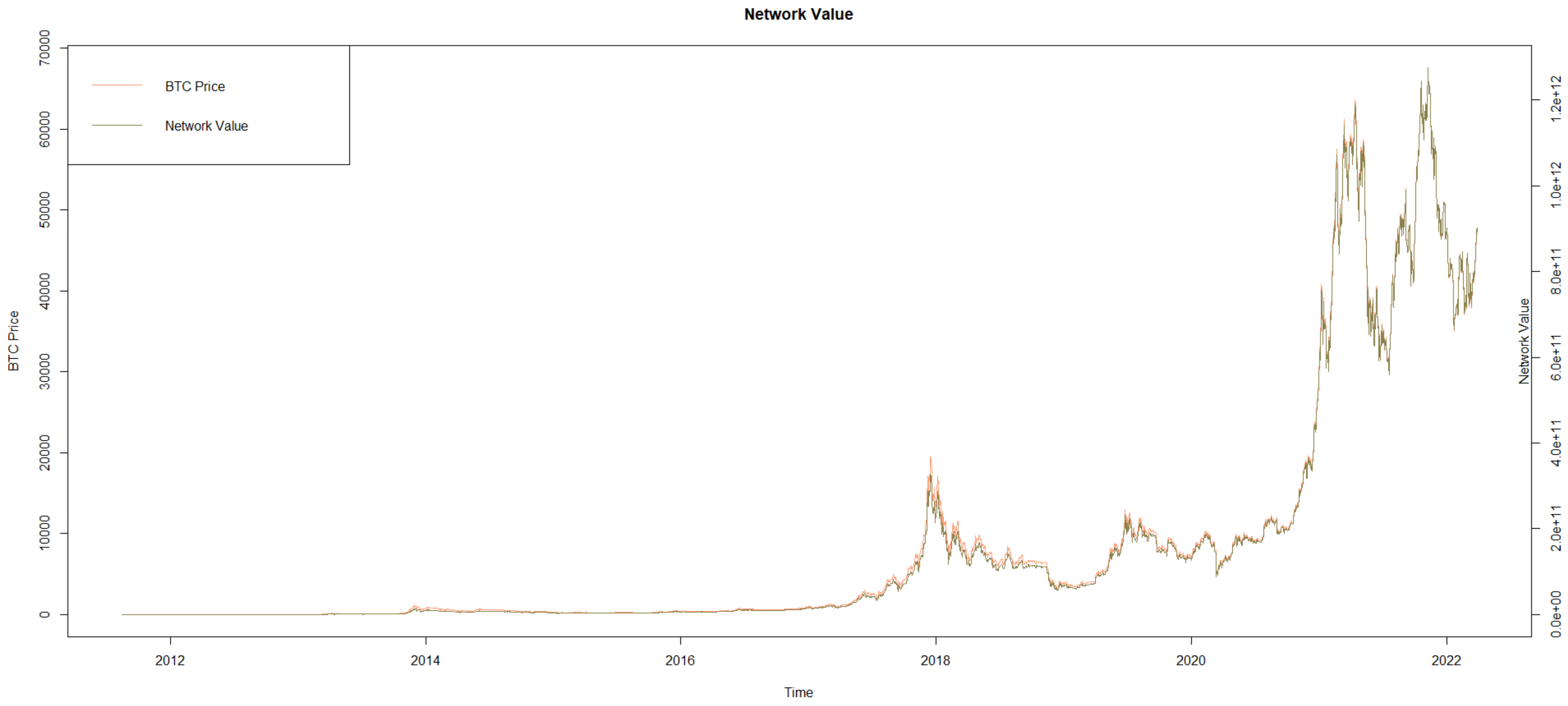
| Network value | USD | Market capitalization |
| Transaction value | USD | The total estimated value of daily transactions on the block chain |
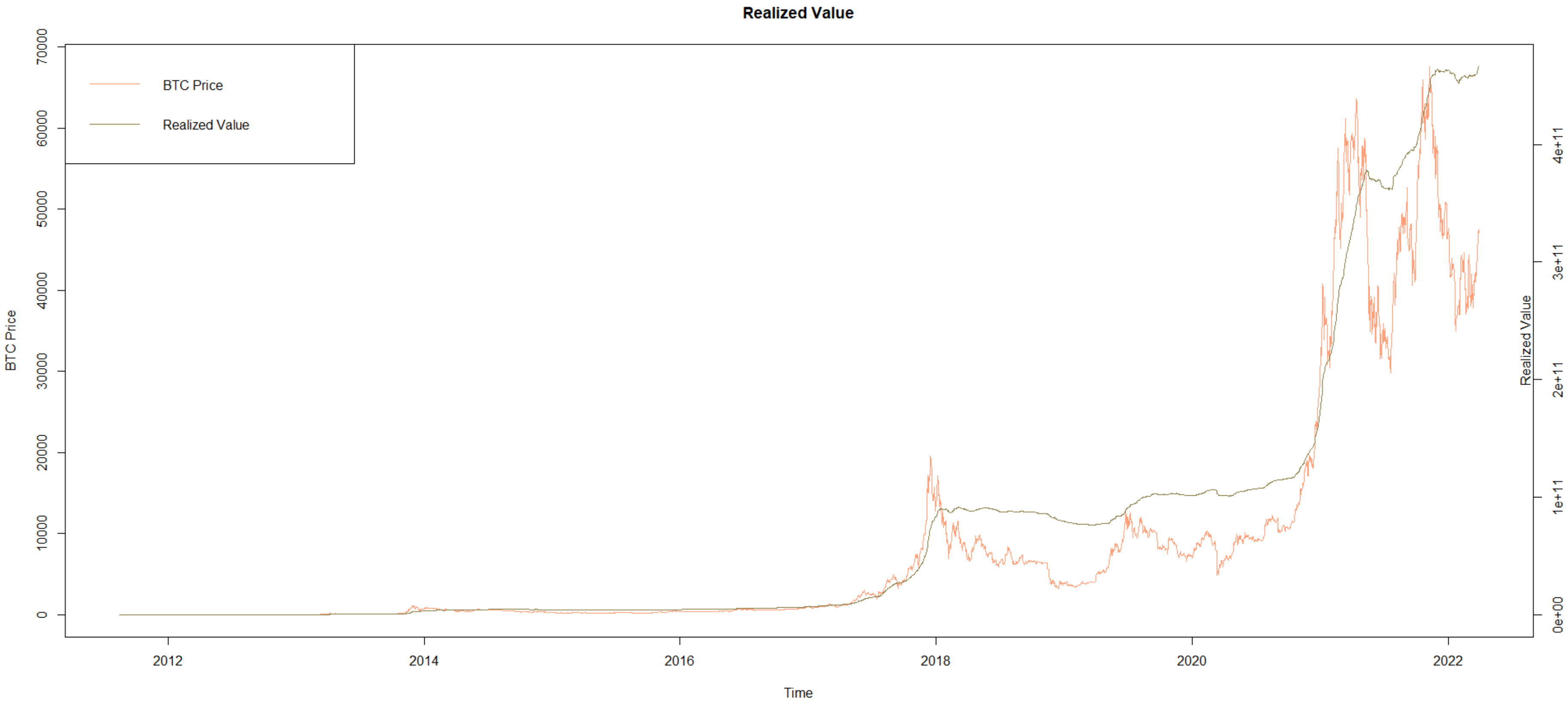
| Realized value | USD | Market capitalization measured by the last trade price of each coin |
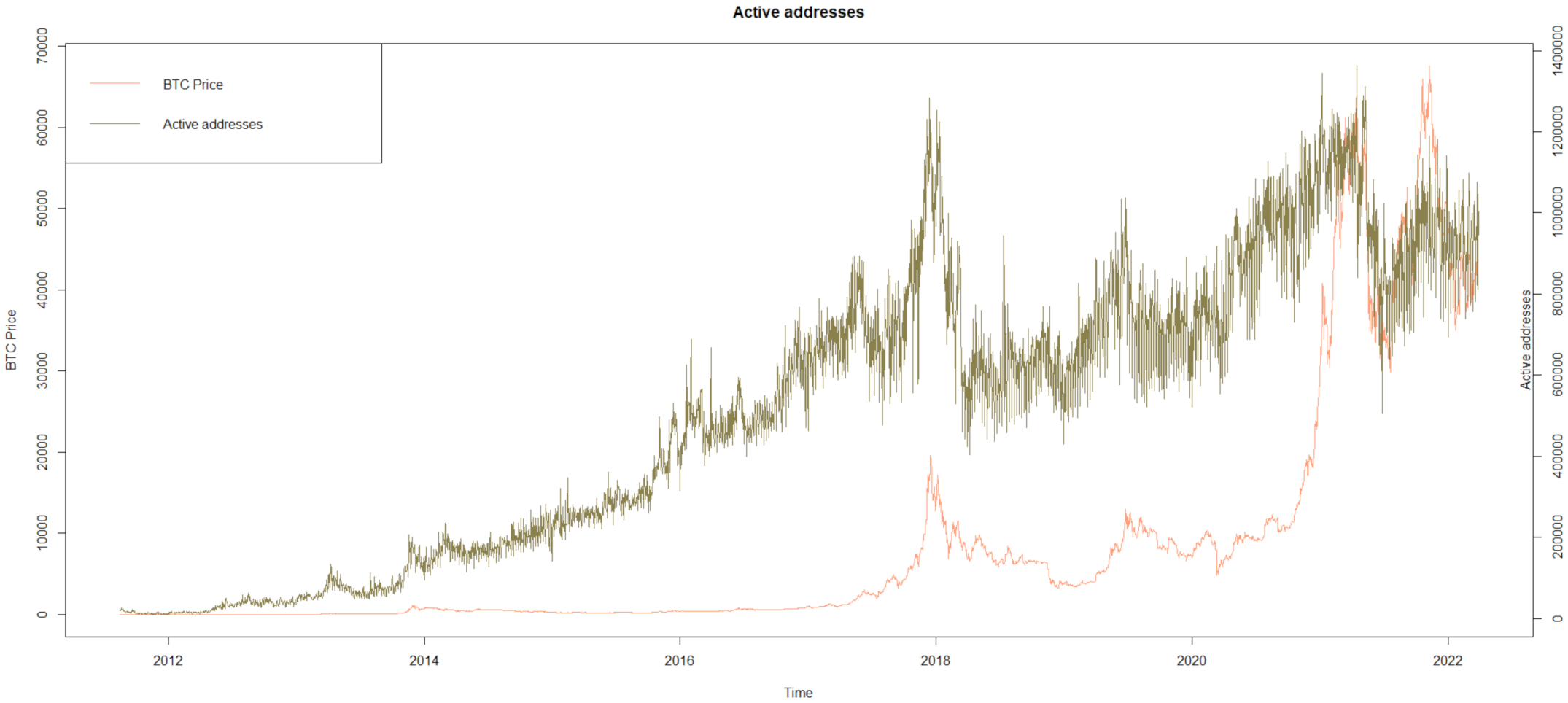
| Active addresses | Number | The number of addresses that were sent or received |
| Network hashrate | Number | The hashrate of the total Bitcoin network |
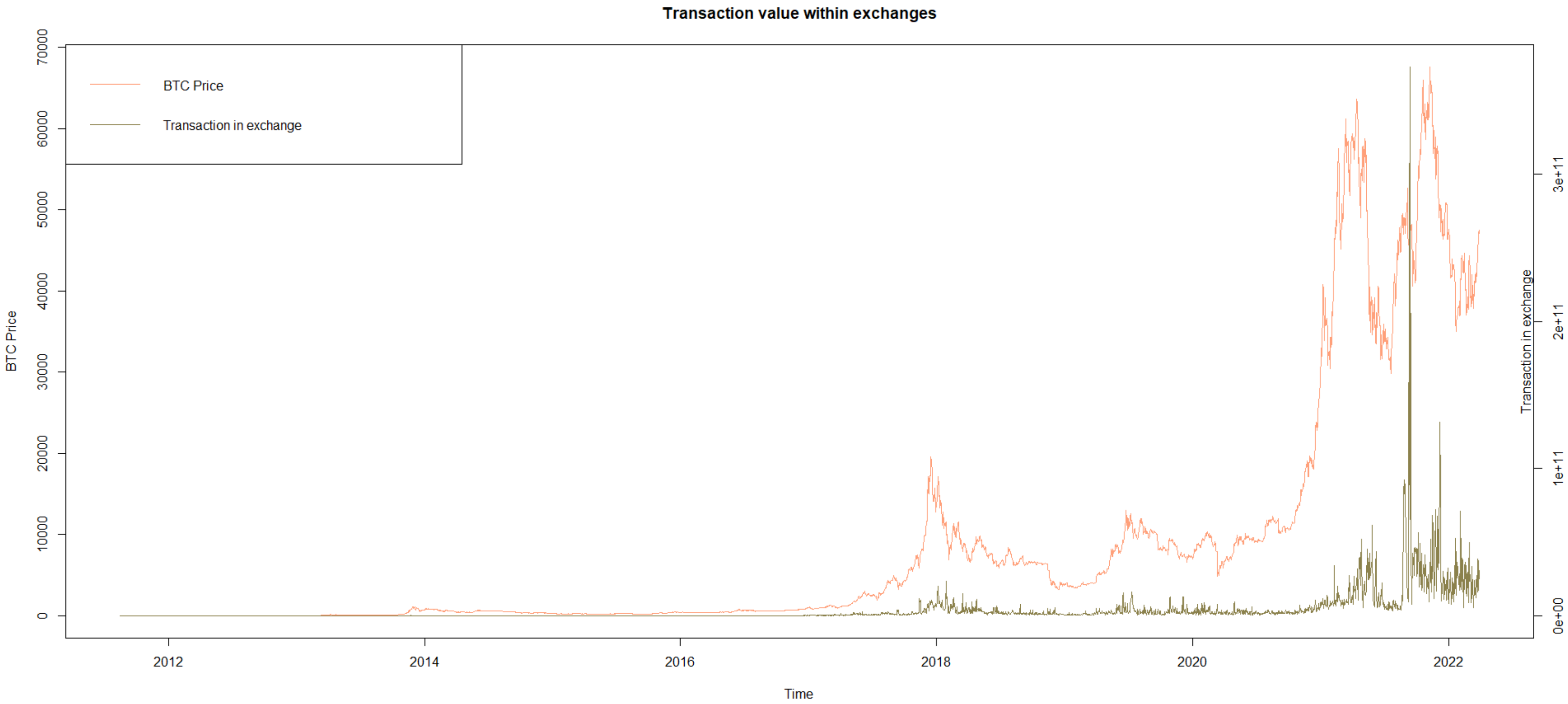
| Transaction in exchanges | Number | The total estimated value of daily transactions within exchanges |
| Risk-free rate | Number | United States 10-year treasury rate |
| BTC (Price) | BTC (Log Returns) | NVTS_Z | NVRV_Z | NVHRS_Z | NVMLS_Z | NVOLS_Z | INETSPE_Z | VOLT | |
|---|---|---|---|---|---|---|---|---|---|
| Mean | 8879.61 | 0.00 | 0.03 | 0.23 | −0.08 | 0.11 | 0.36 | 0.02 | 0.51 |
| Median | 1183.81 | 0.00 | −0.05 | 0.05 | −0.62 | −0.12 | 0.32 | −0.26 | 0.52 |
| Maximum | 67,589.01 | 0.34 | 4.83 | 3.74 | 3.95 | 4.12 | 4.25 | 3.47 | 4.42 |
| Minimum | 4.55 | −0.68 | −5.41 | −3.31 | −3.05 | −3.49 | −3.48 | −2.66 | −3.05 |
| Skewness | 2.16 | −1.48 | 0.18 | 0.27 | 0.70 | 0.37 | 0.21 | 0.87 | 0.12 |
| Kurtosis | 6.60 | 29.00 | 2.49 | 2.38 | 2.43 | 2.32 | 2.28 | 3.53 | 1.99 |
| Jarque–Bera | 4831 | 104,600 | 58 | 102 | 353 | 153 | 106 | 506 | 163 |
| p-value JB | 0.00 | 0.00 | 0.00 | 0.00 | 0.00 | 0.00 | 0.00 | 0.00 | 0.00 |
| KPSS test | 4.36 * | 0.18 | 0.11 | 0.16 | 0.22 | 0.31 | 0.15 | 0.07 | 0.38 |
| Strategy | Net.Trading.PL | Max.Drawdown | Max.Equity | Min.Equity | Ann.Sharpe | Profit.To. Max.Drawdown | Num.Txns |
|---|---|---|---|---|---|---|---|
| NVTS | 86,002 | −97,656 | 147,472 | −1126 | 0.31 | 0.88 | 38 |
| NVRV | 46,685 | −35,065 | 61,577 | −574 | 0.41 * | 1.33 | 15 |
| NVHR | 37,728 | −55,538 | 47,901 | −7636 | 0.20 | 0.68 | 17 |
| NVML | 43,439 | −18,847 | 50,224 | −2739 | 0.47 * | 2.3 | 20 |
| NVOL | 45,589 | −41,460 | 53,747 | −2877 | 0.30 | 1.1 | 18 |
| INET | 49,862 | −16,249 | 58,375 | 0 | 0.55 ** | 3.07 | 104 |
| VOLT | 24,424 | −74,012 | 52,552 | −20,116 | 0.12 | 0.33 | 16 |
| Wright et al. (2014) test for the equality of all Sharpe ratios;p-value: 0.57 | |||||||
| Strategy | Net.Trading.PL | Max.Drawdown | Max.Equity | Min.Equity | Ann.Sharpe | Profit.To. Max.Drawdown | Num.Txns |
|---|---|---|---|---|---|---|---|
| NVTS | 14,412 | −5070 | 14,748 | −1139 | 0.97 ** | 2.84 | 20 |
| NVRV | 10,575 | 2078 | 12,653 | −539 | 0.87 ** | 5.08 | 5 |
| NVHR | 4928 | −1247 | 5334 | −309 | 0.99 ** | 3.94 | 11 |
| NVML | 1348 | −855 | 2195 | −171 | 0.52 * | 1.57 | 8 |
| NVOL | 1078 | −719 | 1755 | −512 | 0.40 | 1.49 | 9 |
| INET | 8798 | −2078 | 10,876 | 0 | 0.72 ** | 4.23 | 63 |
| VOLT | −109 | −690 | 147 | −547 | −0.08 | −0.16 | 4 |
| Wright et al. (2014) test for the equality of all Sharpe ratios;p-value: 0.10 | |||||||
| Strategy | Net.Trading.PL | Max.Drawdown | Max.Equity | Min.Equity | Ann.Sharpe | Profit.To. Max.Drawdown | Num.Txns |
|---|---|---|---|---|---|---|---|
| NVTS | 32,014 | −36,974 | 33,052 | −6059 | 0.47 | 0.87 | 12 |
| NVRV | 32,119 | −32,552 | 52,609 | −2009 | 0.53 | 0.98 | 6 |
| NVHR | 27,986 | −48,321 | 52,183 | −1360 | 0.35 | 0.58 | 7 |
| NVML | 60,025 | −22,965 | 64,808 | −6758 | 0.77 * | 2.61 | 11 |
| NVOL | 67,803 | −65,104 | 99,413 | −6675 | 0.51 | 1.04 | 10 |
| INET | 25,554 | −18,611 | 28,727 | −4749 | 0.50 | 1.37 | 58 |
| VOLT | 35,319 | −97,656 | 87,840 | −11,490 | 0.21 | 0.36 | 8 |
| Wright et al. (2014) test for the equality of all Sharpe ratios;p-value: 0.87 | |||||||
| Strategy | Net.Trading.PL | Max.Drawdown | Max.Equity | Min.Equity | Ann.Sharpe | Profit.To. Max.Drawdown | Num.Txns |
|---|---|---|---|---|---|---|---|
| NVTS | 90,167 | −84,680 | 131,147 | −1825 | 0.36 | 1.06 | 51 |
| NVRV | 56,476 | −78,834 | 94,966 | −2749 | 0.24 | 0.72 | 20 |
| NVHR | 58,045 | −17,061 | 58,434 | −7471 | 0.59 ** | 3.40 | 26 |
| NVML | 64,323 | −26,204 | 65,491 | −2788 | 0.45 * | 2.45 | 24 |
| NVOL | 65,536 | −80,873 | 104,576 | −7520 | 0.29 | 0.81 | 24 |
| INET | 38,272 | −18,715 | 49,711 | −1415 | 0.39 ** | 2.04 | 238 |
| VOLT | 8171 | −80,873 | 48,166 | −32,706 | 0.04 | 0.10 | 17 |
| Wright et al. (2014) test for the equality of all Sharpe ratios.p-value: 0.36 | |||||||
Publisher’s Note: MDPI stays neutral with regard to jurisdictional claims in published maps and institutional affiliations. |
© 2022 by the authors. Licensee MDPI, Basel, Switzerland. This article is an open access article distributed under the terms and conditions of the Creative Commons Attribution (CC BY) license (https://creativecommons.org/licenses/by/4.0/).
Share and Cite
Yang, Z.; Fantazzini, D. Using Crypto-Asset Pricing Methods to Build Technical Oscillators for Short-Term Bitcoin Trading. Information 2022, 13, 560. https://doi.org/10.3390/info13120560
Yang Z, Fantazzini D. Using Crypto-Asset Pricing Methods to Build Technical Oscillators for Short-Term Bitcoin Trading. Information. 2022; 13(12):560. https://doi.org/10.3390/info13120560
Chicago/Turabian StyleYang, Zixiu, and Dean Fantazzini. 2022. "Using Crypto-Asset Pricing Methods to Build Technical Oscillators for Short-Term Bitcoin Trading" Information 13, no. 12: 560. https://doi.org/10.3390/info13120560
APA StyleYang, Z., & Fantazzini, D. (2022). Using Crypto-Asset Pricing Methods to Build Technical Oscillators for Short-Term Bitcoin Trading. Information, 13(12), 560. https://doi.org/10.3390/info13120560