Article

A Missing Data Compensation Method Using LSTM Estimates and Weights in AMI System

1
Kepco Kdn Co., Ltd., 661, Bitgaram-ro, Naju-si 58322, Korea
2
Department of Computer Engineering, Chosun University, 309, Pilmun-daero, Dong-gu, Gwangju 61452, Korea
*
Author to whom correspondence should be addressed.
Information 2021, 12(9), 341; https://doi.org/10.3390/info12090341
Submission received: 29 July 2021 / Revised: 11 August 2021 / Accepted: 13 August 2021 / Published: 24 August 2021

Abstract

:
With the expansion of advanced metering infrastructure (AMI) installations, various additional services using AMI data have emerged. However, some data is lost in the communication process of data collection. Hence, to address this challenge, the estimation of the missing data is required. To estimate the missing values in the time-series data generated from smart meters, we investigated four methods, ranging from a conventional method to an estimation method applying long short-term memory (LSTM), which exhibits excellent performance in the time-series field, and provided the performance comparison data. Furthermore, because power usages represent estimates of data that are missing some values in the middle, rather than regular time-series estimation data, the simple estimation may lead to an error where the estimated accumulated power usage in the missing data is larger than the real accumulated power usage appearing in the data after the end of the missing data interval. Therefore, this study proposes a hybrid method that combines the advantages of the linear interpolation method and the LSTM estimation-based compensation method, rather than those of conventional methods adopted in the time-series field. The performance of the proposed method is more stable and better than that of other methods.

1. Introduction

Advanced metering infrastructure (AMI) is an essential infrastructure for implementing smart grids, which comprises smart meters, a communication network, meter data management system (MDMS), and an operating system. In addition, modems are installed in the smart meters to facilitate bi-directional communication [1,2]. The AMI operating system enables the convergence of various services such as remote meter reading, demand management, power consumption reduction, and power quality improvement based on a bi-directional communication between consumers and power companies [3]. The Table 1 is shows, Starting with the first phase of the AMI construction project for 2 million households in 2013, with a goal of completing the construction for a total of 22.5 million households by 2020, according to the new energy industry acceleration policy, the Korea Electric Power Corporation (KEPCO) completed the construction of AMI for approximately 6.8 million households by 2018 and 400 households in 2019, thereby handling AMI operations for approximately 10 million households [4]. However, it has become difficult to construct the AMI for all 22.5 million households by 2020, as originally planned.
Once the AMI deployment is totally complete, several new services will be created, helping people’s lives and stimulating several positive changes. For example, via power consumption pattern analysis [4], real-time pricing (RTP) [5], critical peak pricing (CPP) [6], and people’s demand response (DR), various services are expected to appear, which include business hour prediction services for stores and life safety services for the elderly living alone [7]. For the provision of these services, it is crucial to properly acquire meter data from power meters. However, although the current AMI system has guaranteed stable performance in overhead power lines via the continuous improvement of the domestic power line communication (PLC) technology and meter reading procedures, difficulties are experienced in securing stable meter reading performances for underground lines, in which noise and attenuation are severe [8]. Consequently, the monthly and daily meter reading success rates are approximately 98% and 95%, respectively, which are both on the low side. The smart meter may incorporate different technologies such as WiSUN, Zigbee, LTE, and PLC In this way, the device chooses a short range technology to connect and relay packets from other smart meters using multi-hop routing [9]. In South Korea, more than 85% of the communication equipment comprising the AMI adopt PLC networks, and owing to environmental impacts such as signal attenuation, which is a PLC feature, missing values may occur in data owing to errors in the communication process of sending data to servers, such as poor communication or malfunction. Hence, a challenge emerges, as the quality of data declines [10,11]. In this technical background, false metering reading verification and missing value estimation algorithms for meter reading data are significantly critical components that determine the reliability of AMI meter reading data. Therefore, sophisticated algorithms reflecting the characteristics of field data are required [12]. In other words, a data preprocessing method is required to analyze the time-series data collected from smart meters, determine missing values in the smart meter data, and replace them with certain value [13,14,15,16,17,18]. Power meter data are one-dimensional time-series data that reflect the cumulative power consumption according to the time. If a value is lost in time-series data, the missing value circumstance may be defined as the time at which the missing value occurred, the value in the time band before the missing value occurred, and the time and value at the point where data first appeared after the missing value occurred [19]. As shown in Figure 1, In this research, we studied a compensation method for the missing data after the next data appears, following the missing interval, i.e., a method for correcting the data in the state that the data exist, before and after the missing data interval in the middle. The estimation algorithms for the data correction include the most basic linear interpolation method [20,21], similar-past-situation substitution method [22,23], autoregressive integrated moving average (ARIMA) estimation interpolation [24,25] regression equation-based missing data estimation method, B-Spline, non-parametric regression equation-based missing data estimation method [26], least-square method applied with missing data estimation method [27], and estimation method using artificial neural network [28]. In other words, various algorithms are adopted depending on the type of missing data. However, the aforementioned algorithms are not suitable for the power consumption data of KEPCO because they are not linear. Therefore, we conducted comparative experiments on existing estimation methods to increase their accuracy by improving the precision for the missing data intervals, and subsequently proposed a hybrid algorithm that combines their advantages.

2. Related Work

Research on data preprocessing in power systems has been actively conducted in South Korea and other countries. In general, the simplest methods for processing missing data in power systems can be categorized into two types. First, there is a method that adopts linear interpolation, with measurement data adjacent to the missing interval. This method is very simple and highly effective when the interval of omitted data in the measurement data is short. However, if the interval of the omitted data is long, the accuracy may be poor. Second, there is a similar-past-situation substitution method that determines a past situation with a similar pattern in the same time band before the missing data interval, based on the missing time, and harnesses it to replace the missing data. This method is also highly effective when patterns are consistent in the data. However, unlike other types of data, power data do not always have cyclic patterns. Therefore, although this method may be effective in certain datasets that have cyclic patterns, it is not suitable for datasets that have multiple types of power consumption patterns. Experiments are conducted on compensation methods based on ARIMA and long short-term memory (LSTM) estimations, which are compensation methods based on time-series estimation, in addition to these two conventional methods [29]. In this research, we study a hybrid method that combines the advantages of the linear interpolation method and those of the LSTM estimation-based compensation method; subsequently, we perform a comparative analysis.

2.1. Linear Interpolation Method

Research on data preprocessing in the power system field has been actively conducted in South Korea and other countries [30,31]. Among them, the most basic and frequently adopted method is linear interpolation. When the values of two points are given, linear interpolation is a method that linearly estimates the value of a point between them, according to the straight distance.
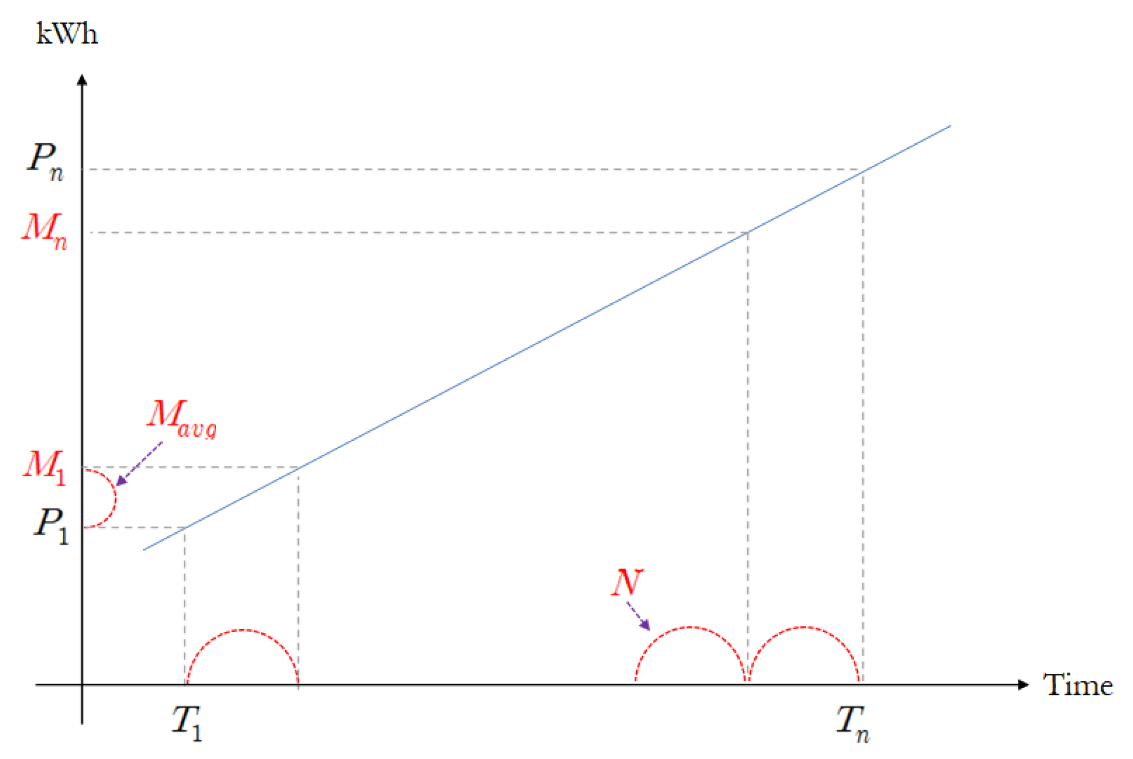
In Figure 2, the X-axes and Y-axes represent the time axis and accumulated power usage, respectively. M denotes the missing data and N represents the number of the missing data intervals; accordingly, M n + 1 . M a v g represents the average power usage for each missing interval.
M a v g = ( P n P 1 ) ÷ N
M 1 = P n + M a v g
M 2 = M 1 + M a v g
...
M n = M ( n 1 ) + M a v g
In the linear interpolation method, the power consumption increases continuously along the time axis, owing to its characteristics. Therefore, suppose the time band before and after the missing data are P 1 and P n , respectively; then it is the same as calculating the accumulated power usage of P n minus the accumulated power usage of P 1 , and dividing it by the number (N) of data in the missing interval.

2.2. Similar-Past-Situation Substitution Method

Unlike other types of data, power consumption data characteristically have inertia. This means that data at a specific point in time are substantially similar to data at a close time point in the past, and they are highly affected. For example, at a typical home, people go to work in the morning and return at night on weekdays. Hence, the power consumption patterns are similar according to time. Based on this idea, this method adopts a similar power consumption pattern of the past to correct the missing data. The most common method adopted when measuring similarity involves calculating the Euclidean distance [32,33].
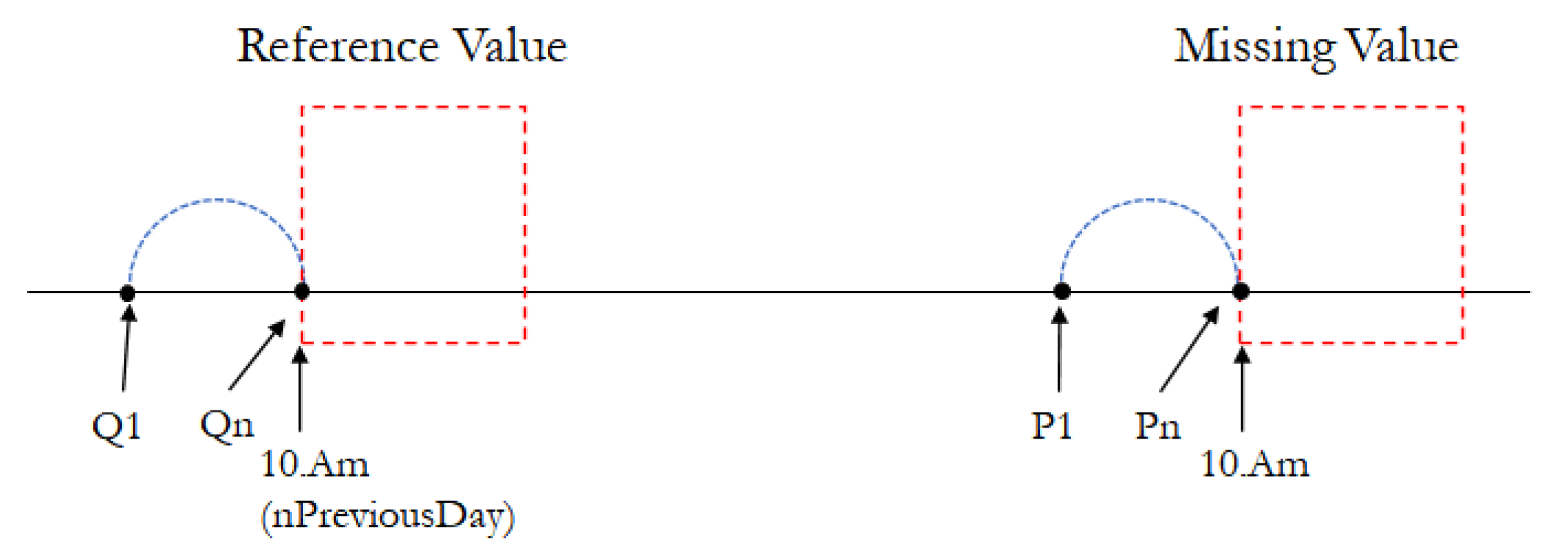
The compensation method of Figure 3 can be expressed in the following equations:
M 1 = P n + R 1
M 2 = M 1 + R 2
...
M n = M ( n 1 ) + R n
M 1 denotes the first missing data, and R 1 represents the consumption in the first interval of a similar situation in the past. Ultimately, the value of M 1 is corrected by calculating the accumulated usage before the missing data ( P n ) plus the value of the first reference consumption in the past similar situation ( R 1 ), and the second missing data ( M 2 ) is corrected by calculating the first corrected data ( M 1 ) + the value of the second reference consumption in a similar past situation ( R 2 ).

2.3. ARIMA Estimation-Based Compensation Method

An ARIMA model generalizes an autoregressive moving average (ARMA) model that adopts previous observations and errors to describe the current time-series value. The ARMA model can be solely applied to stable time-series data, and it solely adopts past data. In contrast, the ARIMA model can be applied even if the analysis target is an unstable time-series, and it can reflect the trend (momentum) of past data. The ARIMA model solely considers its own momentum, and does not consider the that of white noise. This is owing to the absolute absence of momentum in the white noise of a correct model. This method corrects data in the missing interval by estimating the consumption via an ARIMA algorithm. In addition, it can be processed even if the accumulated power usage is adopted as an input value without using the differencing data.

2.4. LSTM Estimation-Based Compensation Method

LSTM is a model created to address the vanishing gradient problem, a limitation of recurrent neural networks (RNN). Unlike conventional RNNs, cell-state was adopted in the memory cells, and three gates (input, output, and forget gates) were adopted to address the vanishing gradient problem. The power usage in the missing interval is estimated using the LSTM model. To correct the first missing data, the estimated interval usage is introduced to the accumulated usage, just before the missing interval. Next, the second estimated data are added to the first corrected missing data to correct the second missing data. Accordingly, the data in the mission interval are sequentially corrected.

3. Comparative Experiments on Missing Data Compensation Methods

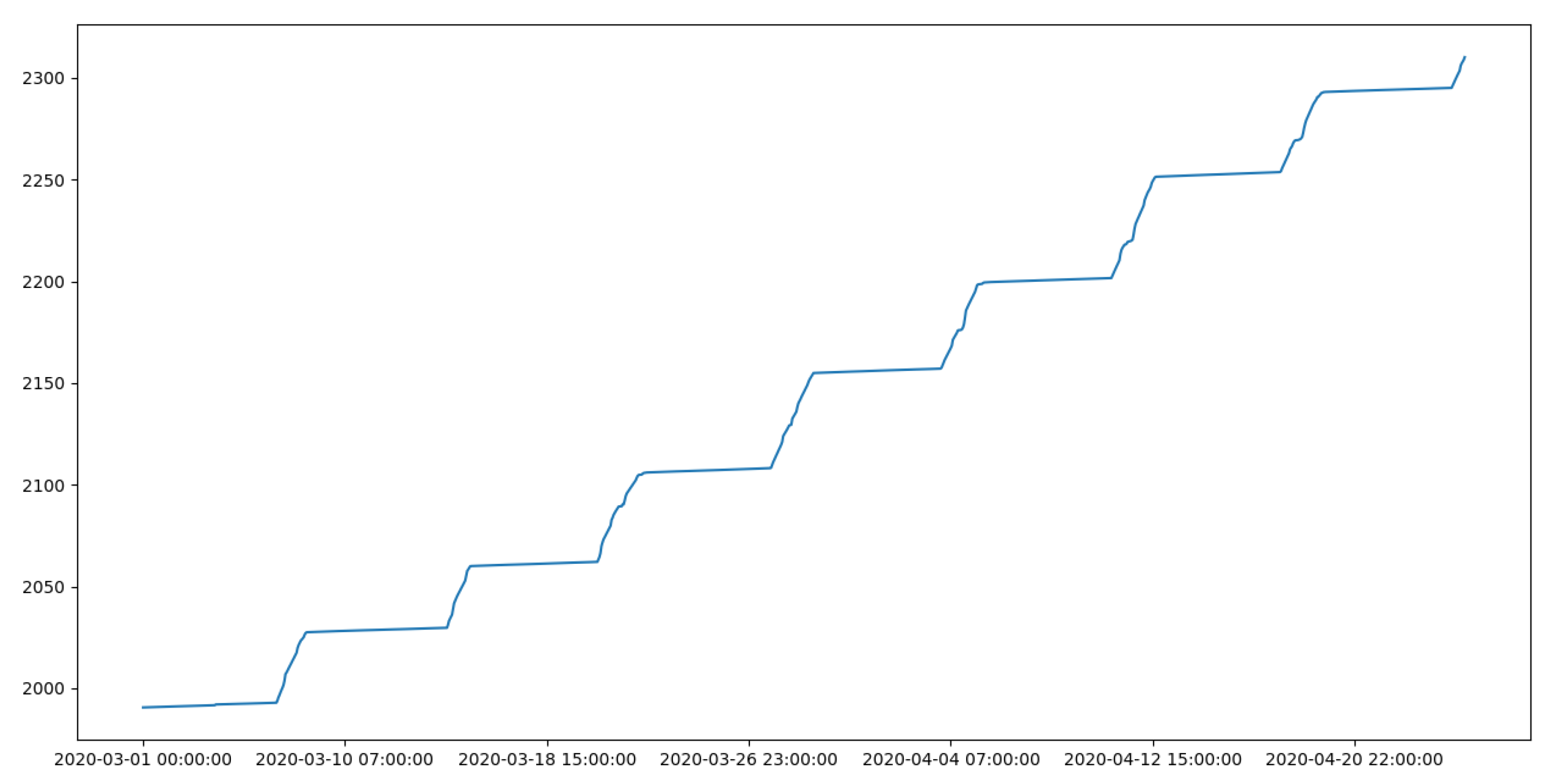
As a power consumption feature, the values in the power consumption data continuously trend upward, as illustrated in Figure 4. Therefore, the interval usage for each hour is calculated using the difference via preprocessing. For example, if the accumulated usage is 950 kWh at 9:00 and 1000 kWh at 10:00, the interval usage at 10:00 is 50 kWh. Preprocessing is performed to calculate the interval usage of all selected target customers, and save it in a separate column.
In data mining, outlier detection refers to the observation of data points or events that indicate more significant differences in values than the majority of data. Therefore, an outlier in smart meter data indicates a case in which the power consumption data measured, using a smart meter at a certain time, is significantly larger or smaller than a comparable average group. There are several types of outlier detection methods; however, because power consumption data are one-dimensional time-series data, this study adopts an outlier detection method of univariate data. In other words, the interval usage is calculated, and in the case of erroneous data, in which the interval usage of the missing data interval in actual data is zero, the pertinent data of the customers are all discarded because they can have negative effects on the experiment.

3.1. Linear Interpolation

Linear interpolation is the simplest, easily applicable method, with a significantly stable effect. It requires a simple calculation using the data collected before the missing interval to correct the missing data.
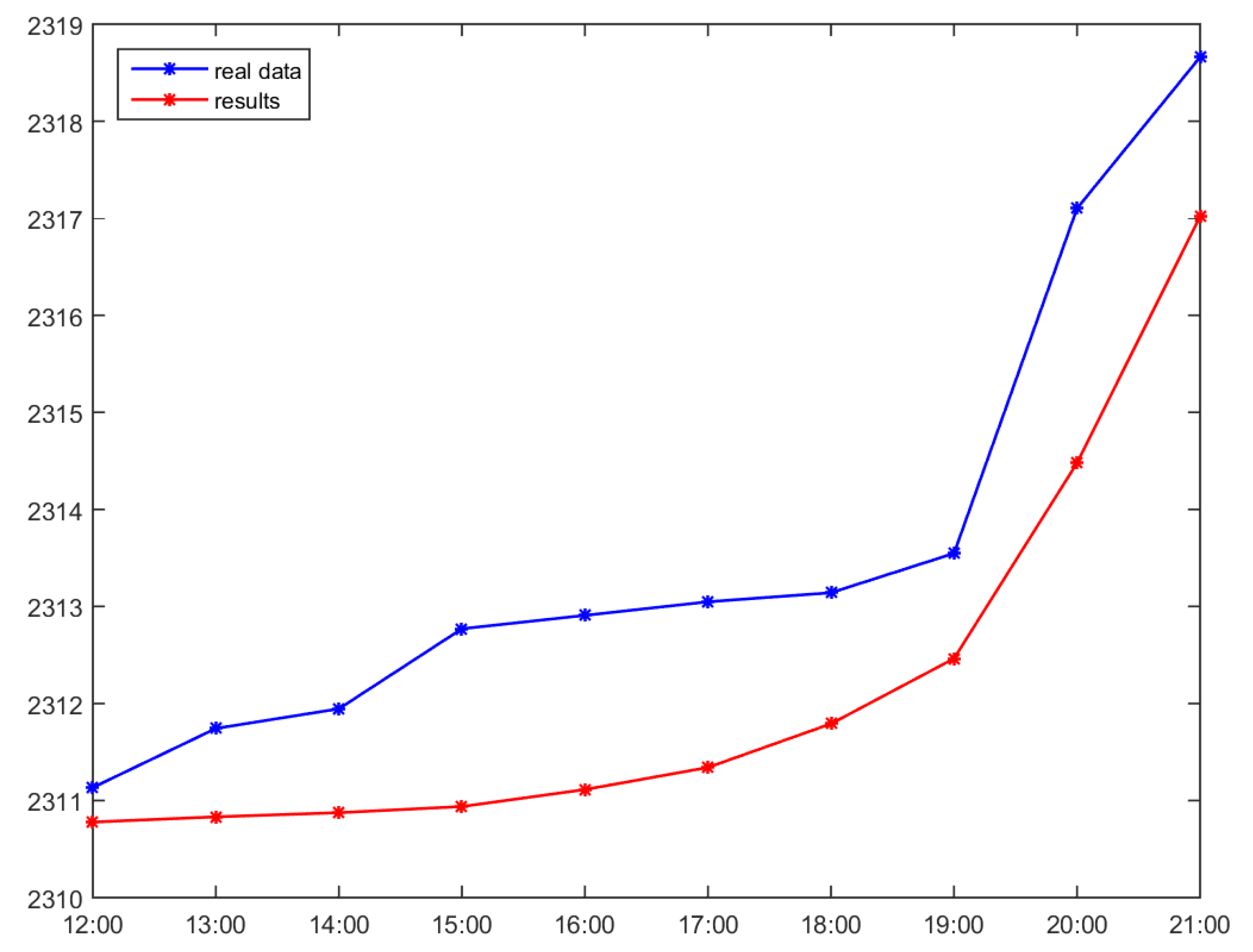
In Table 2, the difference in the accumulated usage was calculated between time periods of 11:00 and 22:00, which were before and after the missing data. Subsequently, the difference (10.474) was divided by the number of missing intervals (11) to obtain the average usage (0.9522). This average usage was added sequentially to the previously accumulated usage of the missing data to correct the missing data.
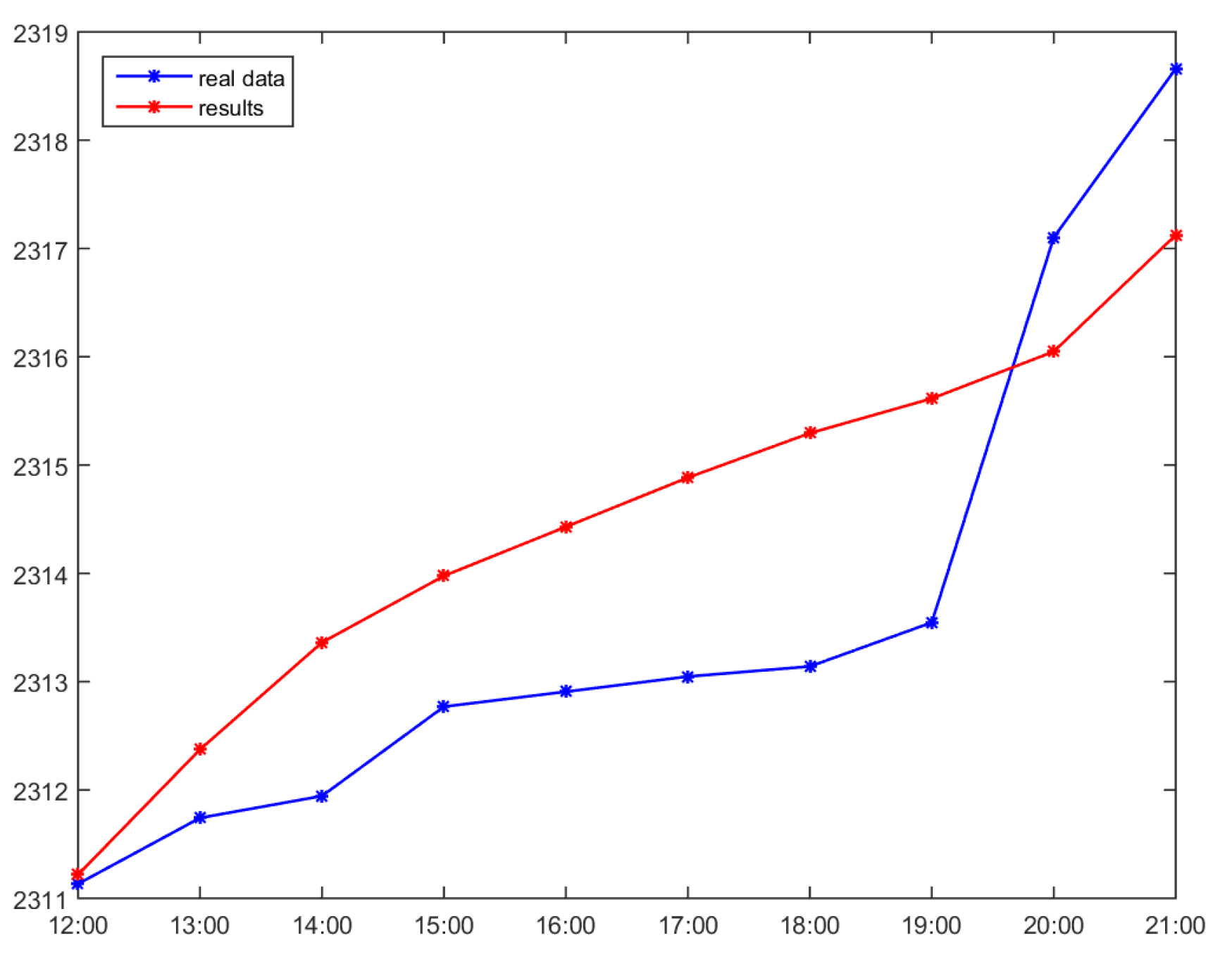
Because the linear interpolation method uniformly divides the missing intervals, the graph is corrected in a straight line. However, because the power consumption is different at each hour in the real data, errors emerge, as illustrated in Figure 5. This linear interpolation method will produce optimal estimates in time bands where the consumption change is uniform. The linear interpolation method facilitates fast and simple calculations, while saving resources such as CPU and memory. As a limitation of this method, severe errors occur in the middle of the missing interval if the consumption is not uniform.

3.2. Similar-Past-Situation Substitution

The similar-past-situation substitution method determines a past situation in which the power usage pattern is similar, and corrects the missing data, using that usage as a reference. To apply this method, first, a similar past situation of individual customers must be determined. As a feature of power data, weekly patterns are similar in terms of working days and holidays. Therefore, we limited the data to seven days before the missing-data day to find a similar situation in the past. For similarity, we adopted the simplest Euclidean similarity to select a date with the smallest error.
Because data were missing between 12:00 and 21:00 on 25 April, we compared the Euclidean similarity with the same time bands of the previous seven days, based on the data of ten previous hours (02:00–11:00). In samples presented in Table 3, because the sum of absolute errors on 18 April was 2.417, which was smaller than that of other dates, we selected that particular date for a similar pattern. In Table 4, if a similar past situation is determined, then the interval usage at the same time period where the missing data occurred is adopted as reference data. In the aforementioned case, the usages in the intervals from 12:00 to 21:00 on 18 April were adopted to correct the data on the data-missing day.
The interval usage in the reference data of the same time band is added to the accumulated usage before the start of the missing data. For the second missing data, the interval usage in the reference data of the same time band is added to the corrected previous accumulated usage.
The sample data presented in Table 5 were corrected by applying the reference data of the same time bands on a past-similar-situation day (18 April) for the missing intervals.
In general, when the past-similar-situation substitution method is adopted, the real and estimated data exhibit similar patterns in the graph because most customers exhibit patterns of using power consistently, depending on specific types of days such as weekdays, weekends, and holidays. However, the differences are large on irregular holidays or when temperature changes abruptly. The Figure 6 presents a graph obtained from the calculation of the absolute error for each missing time band between the real and corrected data. Because the data at the starting point of the missing interval are corrected by adding the interval usage of the past similar time point, errors are accumulated as the correction work progresses over time, thus increasing the accumulated error. Furthermore, the last corrected data in the missing data interval may become larger than the first data appearing after the end of the missing data interval. In this case, if it is used to correct the power usage data, a critical error will occur owing to a negative value.

3.3. ARIMA Estimation-Based Compensation Method

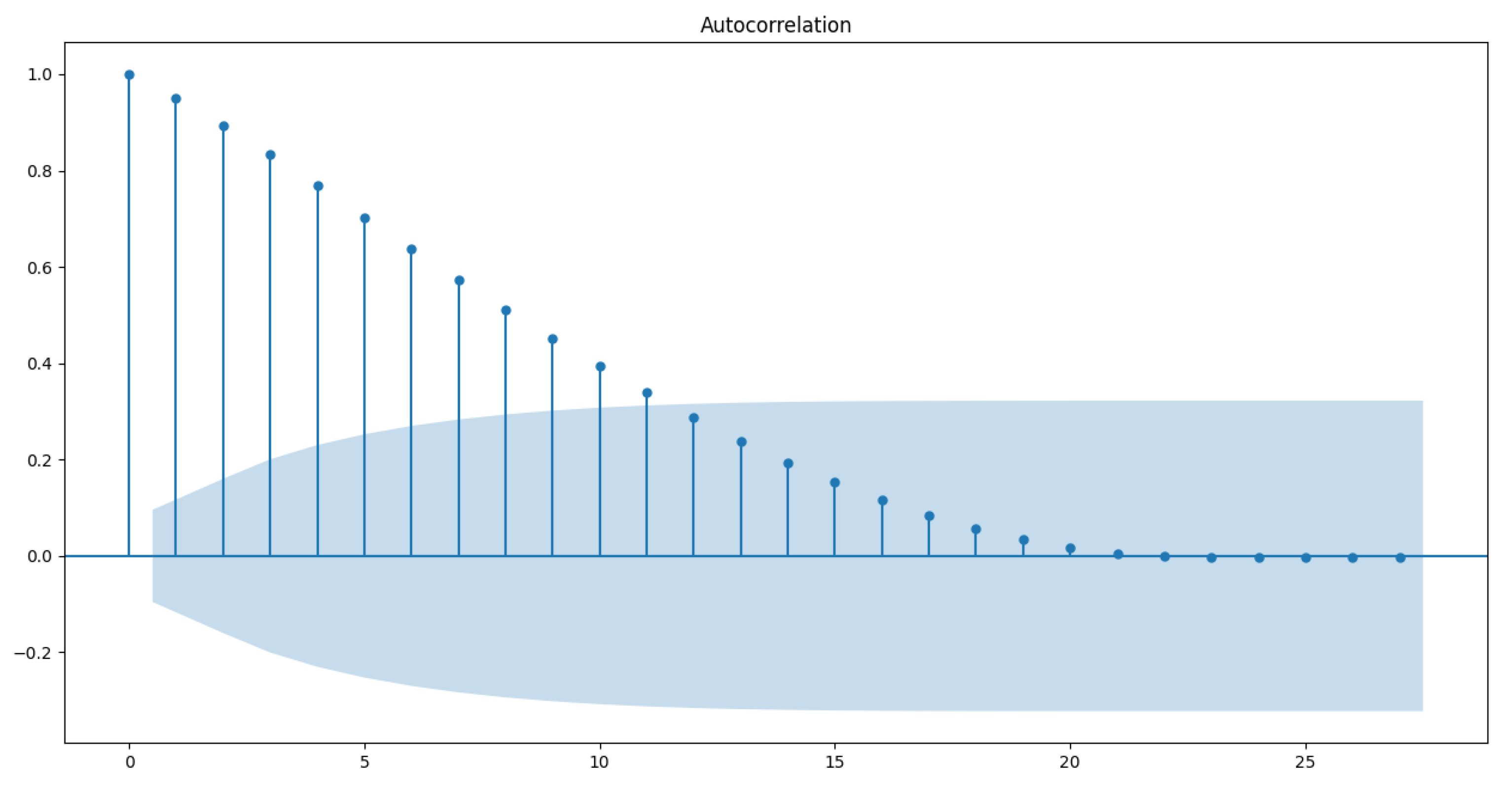
The estimation method using the ARIMA algorithm, which is a conventional time-series estimation method, exhibits a substantially optimal performance in the time series field. To perform the AIRMA time-series estimation, we adopted a method that involves inputting the previous seven-day data of the missing data interval to train the model and estimate the data in the missing value interval. To apply the ARIMA model, we entered the real data as they were, instead of using the interval usages. If the first data differencing is performed by setting “d” of the ARIMA model to “1,” then the data will satisfy the normality. To determine the ARIMA model, we performed a process to determine the p, d, and q values by using the acf() and pacf() functions. As illustrated in Figure 7, the results obtained from the autocorrelation function (ACF) exhibit an exponentially decreasing graph. Therefore, we selected the AR model.
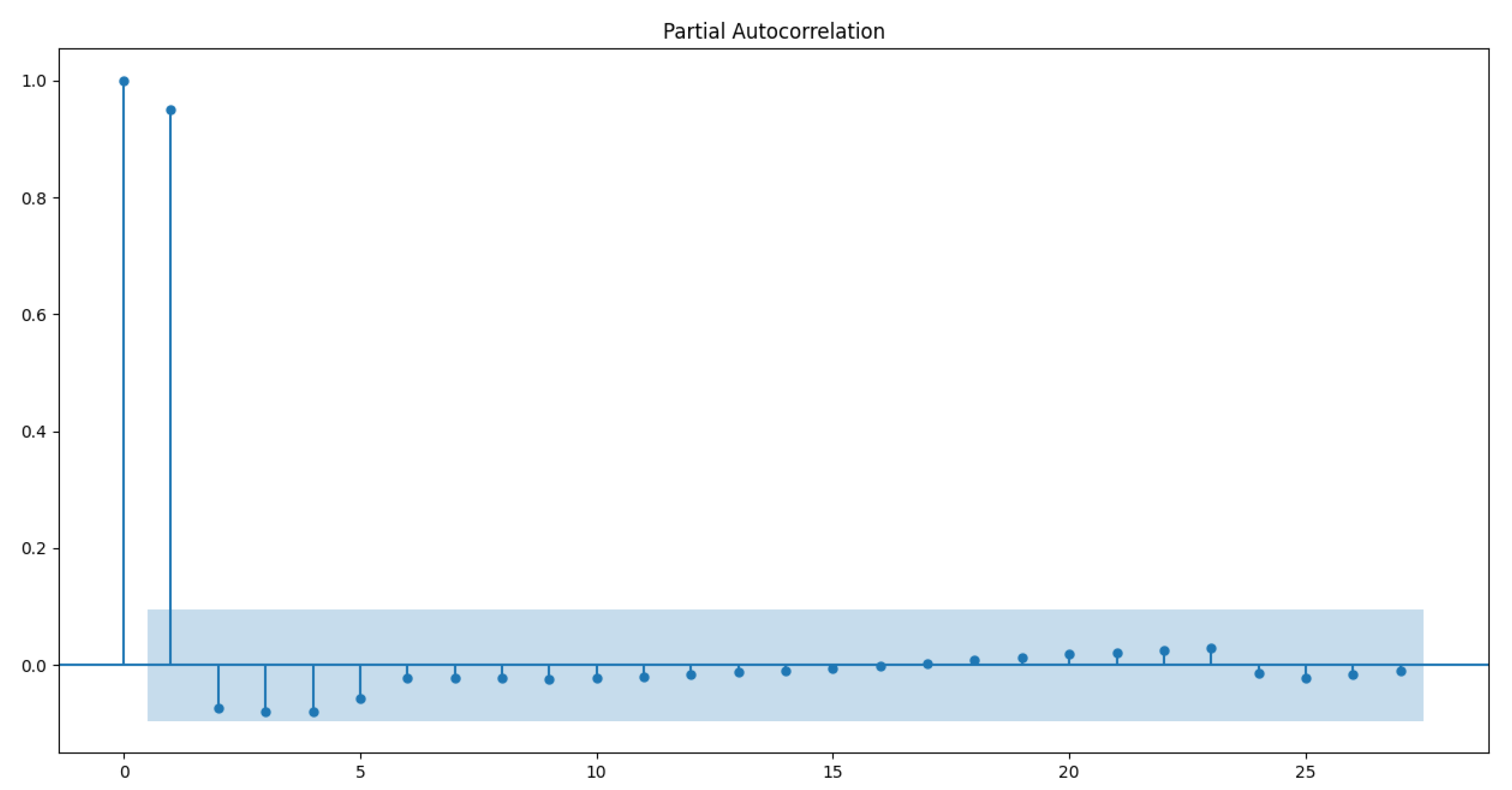
The results of the partial autocorrelation function (PACF) exhibit a cut shape after the second, as illustrated in Figure 8. Therefore, we set the p value of the AR model to “2”.
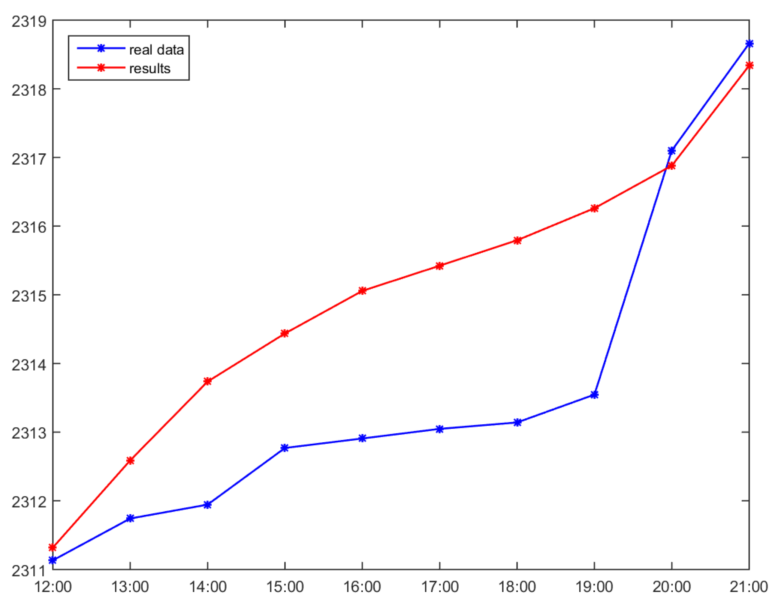
Finally, the p, d, and q values of the ARIMA model were set as: p = 2, d = 1, and q = 0. Table 6 presents the results obtained from correcting the missing data by applying the ARIMA model.
Figure 9 presents a comparison graph of the real data and the results corrected by estimating the missing data via the ARIMA model. The obtained results were substantially optimal in the time-series data. However, the estimation results exhibited a graph shape similar to that obtained from the results of the linear interpolation method.
The figure below presents a graph obtained from calculating the absolute error for each time band of missing data between the real and corrected data. The differences are irregular, and not uniform. Furthermore, the last corrected data in the missing data interval may become larger than the first data appearing after the end of the missing data interval. In this case, if it is used to correct the power usage data, a critical error will occur owing to a negative value.

3.4. LSTM Estimation-Based Compensation Method

We combined a convolutional neural network (CNN) and an LSTM model to estimate the time-series power usages and correct the missing data. We adopted two-week data as the input data and set the window size to 24, which was for one day. The model was set up by mixing in the order: CNN layer LSTM layer Dense layer. The experiments were conducted in the environment presented in Table 7. Regarding the LSTM and CNN, we adopted the Tensorflow library in the experiments.
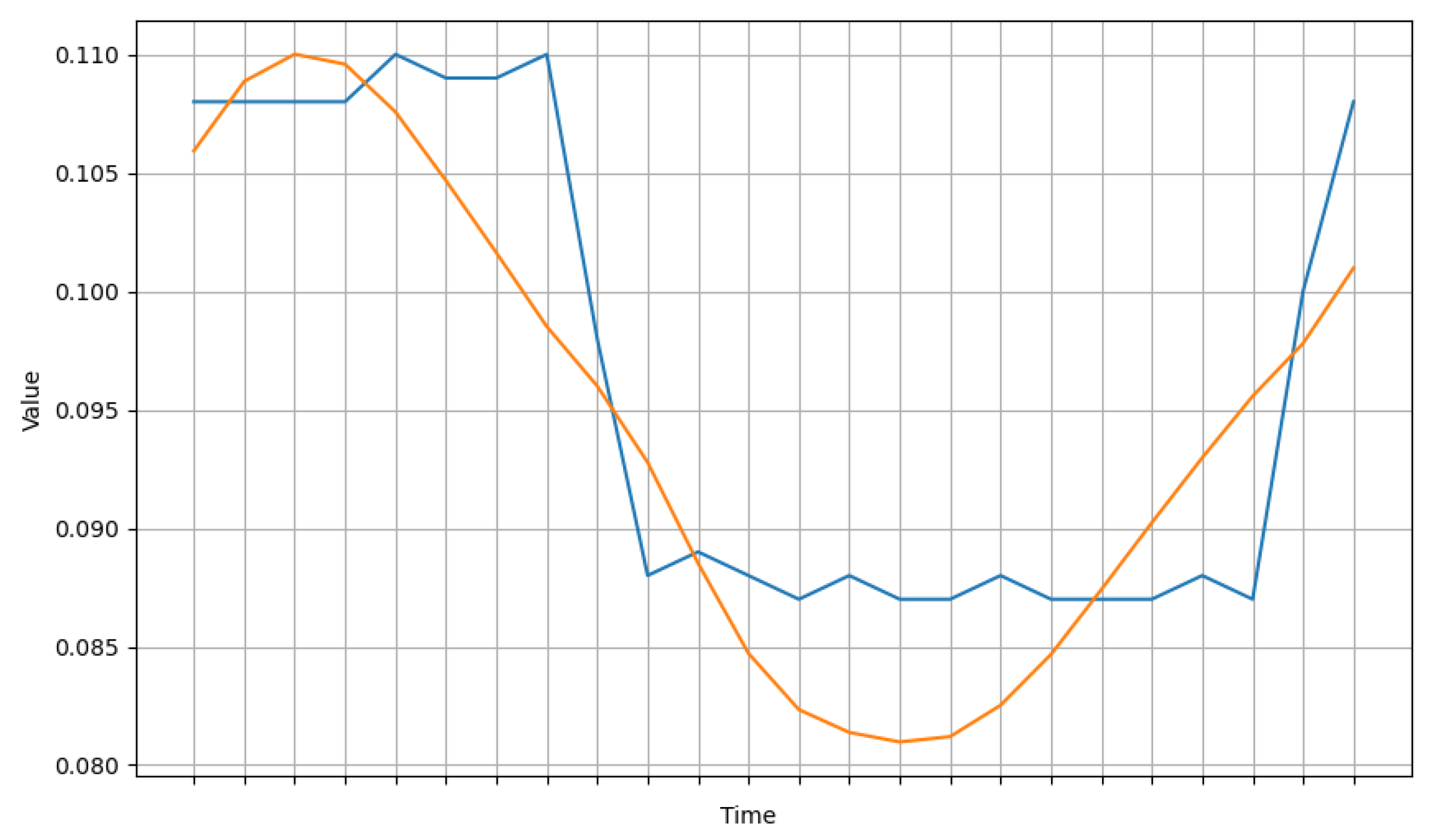
The graph in Figure 10 presents a comparison between the real and estimated result data of the sample customers.
The 24-h data were estimated and compared with the real data. The mean absolute error (MAE) was 0.0056. The number of CNN filters was set to 120, while the number of neurons in the LSTM model was set to 30. Then, they were combined with dense layers, for which the numbers were set to 30, 10, and 1, respectively, to create the model. The number of epochs was set to 20. A total of 713 was trained, and approximately 30 min was required to estimate the result.
We adopted the interval usage data as the input data in the LSTM model, for which the first differencing of the cumulative data was performed. After training via the LSTM model, we estimated the missing data. Here, the estimated data were the usage data of the 24-h interval. Table 8 presents the estimated values of the LSTM interval usage.
To correct the LSTM estimated value, the estimated interval usage of the first time band was added to the accumulated power usage of the previous time band before the start of the missing data, which was the first accumulated usage. Next, the second estimated value was added to the first corrected data to correct the second data. Accordingly, the data in the missing intervals were sequentially corrected.
In Figure 11, the data corrected via the LSTM estimation are significantly similar to the real data. The graph below shows the MAE values, and the errors are not uniform, but relatively jagged. Several experiments were conducted, and the correction based on the LSTM estimation was highly effective. However, the last corrected data in the missing data interval may become larger than the first data appearing after the end of the missing data interval. In this case, if it is used to correct the power usage data, a critical error will occur owing to a negative value.

3.5. LSTM Estimate and Weight-Applied Compensation Method

To this point, we have adopted four methods (linear interpolation, past-similar-situation substitution, ARIMA time-series estimation-based compensation, and LSTM estimation-based compensation methods) to correct the missing data. All three methods, except for the linear interpolation, estimated the power usage to perform the data correction, without considering the first data appearing after the end of the missing interval. In particular, the past-similar-situation substitution and LSTM estimation-based compensation methods estimated the interval usage, rather than the accumulated power usage, and added it to the accumulated power usage of the previous time band of the missing interval to perform the correction; therefore, the error was bound to gradually increase over time. To address this limitation, we propose an LSTM estimate and weight-applied compensation method to improve stability and accuracy. We improved accuracy by applying a weight to the interval usage of each time band estimated via the LSTM estimation, which exhibited the best performance among the aforementioned four methods.
Figure 12 shows the concept of missing data intervals. The procedure of the LSTM estimate and weight-applied compensation method is presented as follows. First, the usage in the missing data interval is estimated via the LSTM estimation. Second, a weight is applied to the estimation result to recalculate the interval usage. Third, the weight-applied interval usage is added to the previous accumulated usage before the occurrence of the missing data. Then, the second weight-applied interval usage is added to the first corrected missing data to correct the second missing data. Accordingly, all data in the missing intervals are corrected. The following equation applies a weight to the interval usage ( D x ) estimated via the LSTM estimation to recalculate the interval usage.
D w ( x ) = ( R s R f ) × D x x = 1 n D x
In the final step, the missing data correction method adds the weight-applied interval usage ( D w n ) to the accumulated usage, before the occurrence of the missing data ( R 1 ), to correct the first value ( M 1 ) of the missing data.
M 1 = R f + D w 1
M 2 = M 1 + D w 2
M n = M ( n 1 ) + D w n
In the following Table 9, the data (LSTM Estimated) obtained via the LSTM estimation was used to calculate the rate for each time band (LSTM TermRate). If the difference is calculated between the accumulated power usage that first appears after the end of the missing interval ( R 2 ) and the accumulated usage just before the start of the missing interval ( R 1 )), the total power usage in the missing interval is determined. If the total power usage value is multiplied by the rate for each time band (LSTM TermRate), then the final interval usage for each band of the missing data interval is determined (Weight LSTM Usage).
Algorithm 1 is missing data compensation algorithm that applied weighted LSTM model. First of all, a list of meters with missing data needs to be set. The next step is to calculate the interval power usage using the accumulated power usage of each meter. The interval usage can be estimated by giving it to LSTM model as an input. Each TermRate is calculated by applying a weight to the each interval usage estimates derived from LSTM model to recalculate to recalculate the interval usage. The total usage from Rs to Rf, (Rs-Rf) from the equation, multiplied by TermRate equals the weight-applied interval usage. ResultData are created by adding weighted interval usage to real data just before missing subsequently.
Algorithm 1 Weighted LSTM Processing
Input: MeterList
Output: ResultDataPool
  Definition 1. :  Rf—Fisrt real data(real data just before missing)
         Rs—Second real data(first real data after missing termination)
   I n i t a l i z e l i s t T m p R e t P o o l ;
   R E A D M e t e r L i s t w i t h M i s s i n g V a l u e s ;
  for all attribute M I D M e t e r L i s t   do
     A c c u m u l a t e d U s a g e = A c c u m u l a t e d U s a g e D B . g e t v a l u e ( M I D ) ;
     I n t e r v a l U s a g e = C O M P U T E I n t e r v a l U s a g e b y t i m e u s i n g A c c u m u l a t e d U s a g e ;
     L S T M _ I n t e r v a l U s a g e = L S T M _ m o d e l . e s t i m a t e ( I n t e r v a l U s a g e ) ;
     S u m _ L S T M _ I n t e r v a l U s a g e = L S T M _ I n t e r v a l U s a g e ;
     T m p R e t = R f ;
    for all attribute E I U L S T M _ I n t e r v a l U s a g e   do
         W e i g h t e d _ U s a g e = ( R s R f ) × E I U ÷ S u m _ L S T M _ I n t e r v a l U s a g e ;
         T m p R e t = T m p R e t + W e i g h t e d _ U s a g e ;
         T m p R e t P o o l = T m p R e t P o o l . p u t v a l u e ( T m p R e t ) ;
    end for
     R e s u l t D a t a P o o l = R e s u l t D a t a P o o l . p u t v a l u e ( T m p R e t P o o l ) ;
    ClearTmpRet
  end for
Finally, the final interval usage at 12:00 was added to the accumulated power usage, at the time (11:00) before the start of the missing interval, to correct the accumulated power usage (Weighted LSTM Estimated) at 12:00. Next, the estimated value at 13:00 was added to the corrected data of 12:00 to correct the data at 13:00. Accordingly, the data in the missing intervals were sequentially corrected. Figure 13 compares the real data and the data corrected by applying the weight to the data estimated via the LSTM. It is evident that the results are significantly better than the data corrected via the LSTM estimation.
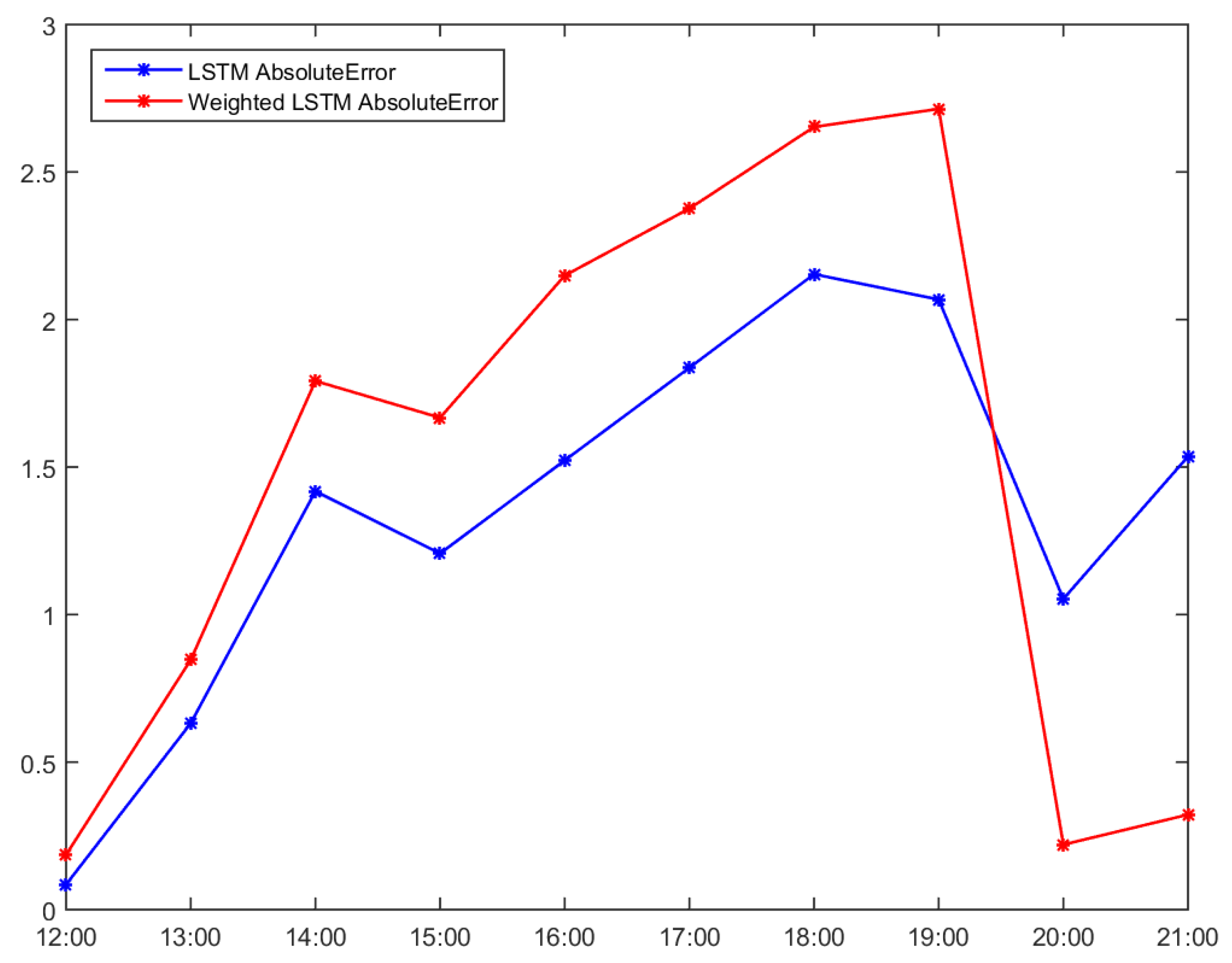
Furthermore, the graph below presents the MAE values of the data corrected by applying the weights to the data estimated via the LSTM. It can be deduced that the errors at the starting and ending points of the missing intervals converge to zero. In other words, the advantage of the linear interpolation method is demonstrated. Furthermore, the errors at the middle time bands are smaller than those of other compensation methods, which represents the advantage of the LSTM estimation-based compensation method.

3.6. Experimental Results

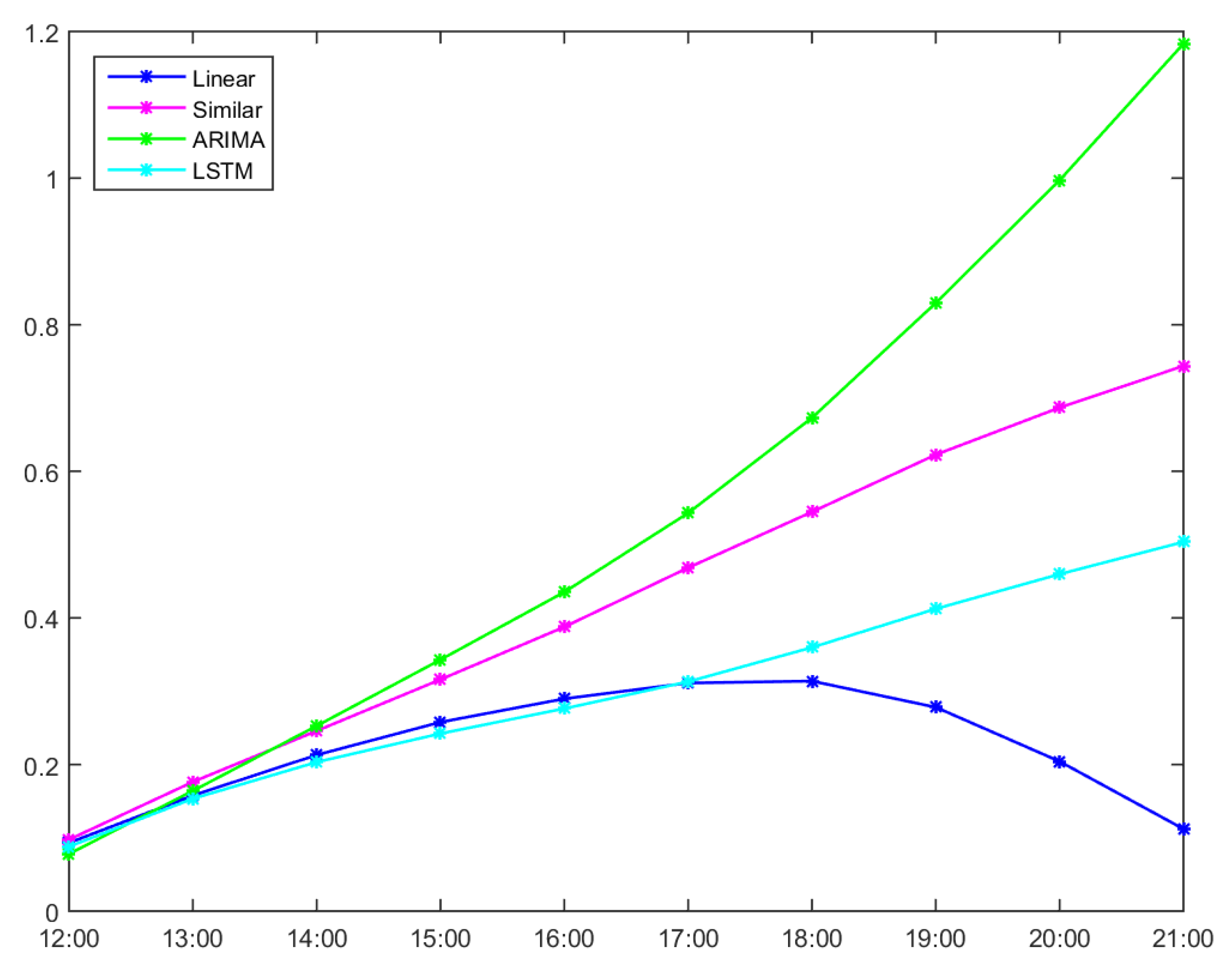
We created a diagram to compare the errors in the aforementioned experimental results between each method (the linear interpolation, past-similar-situation substitution, ARIMA estimation-based compensation, and LSTM estimation-based compensation methods) to investigate and summarize the comparison situation, according to each result. Figure 14 presents the analysis results of the four methods. In all the methods, excluding the linear interpolation method, the MAE value increases over time. The errors increase continuously because the value corrected via the estimation is added to the accumulated value of the previous time band. However, the linear interpolation method exhibits a graph shape, in which the error is smallest before and after the missing interval, because the data before and after the missing interval are differenced and used. Therefore, the linear interpolation exhibits the best results among the four experiments. The second-best performance is presented when the LSTM is applied to estimate and correct the interval usage. Today, LSTM is frequently used, as it provides optimal results in the time-series field. However, in the cumulative power consumption estimation field, it does not exhibit better results than the linear interpolation method.
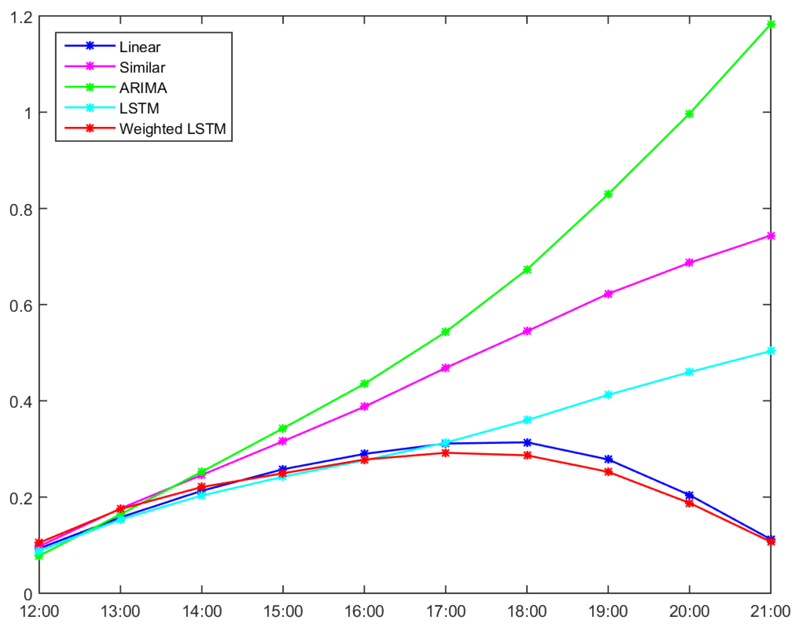
As illustrated in Figure 14, the LSTM estimation-based compensation method exhibited slightly better results, in a number of middle parts, than the linear interpolation method. However, all the other methods, except the linear interpolation method, indicate that the estimated results were sometimes larger than the data collected at 22:00, which were the first data appearing after the end of the missing data interval. In fact, 303 customers exhibited such a case of flipped accumulated usages. The performance of the LSTM estimation-based compensation method may be beneficial to some; however, it cannot be used when the case of flipped accumulated usages occurs, as will trigger a critical error where a negative value of the power usage occurs. As aforementioned, because the limitation of the linear interpolation method could not be addressed, we proposed and tested a hybrid method that combines the advantages of the linear interpolation and LSTM estimation-based compensation methods. Based on Table 10, we can infer that the MAE of the method proposed (Weight LSTM) in this study is the smallest.
Because the advantages of the linear interpolation and LSTM estimation-based methods have been combined, the errors at both ends of the starting and ending parts of the missing data converge to zero, which is the advantage of the linear interpolation, as illustrated in Figure 15. Furthermore, the advantage of the LSTM estimation is applied in the middle time band parts, thus supplementing severe errors in the middle parts, a limitation of the linear interpolation.
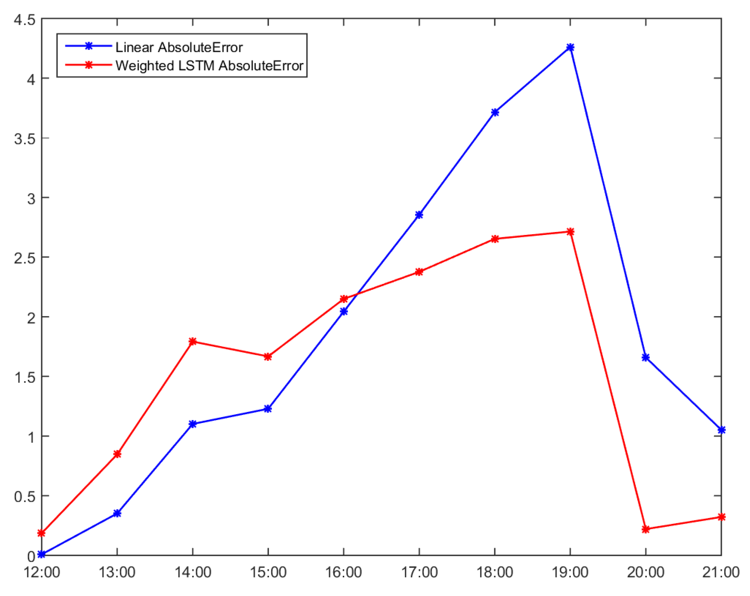
Figure 16 presents a graph that compares the errors between the cases of adopting the LSTM estimate and weight-applied compensation method and the linear interpolation method. The linear interpolation method exhibits the largest error at 19:00; however, the LSTM estimate and weight-applied compensation method exhibits significantly mitigated errors in the middle part.
Figure 17 presents a comparison graph between the LSTM estimation-based compensation method and the LSTM estimate and weight-applied compensation method. The LSTM estimation-based compensation method exhibits optimal results in some time bands; however, after 20:00, the LSTM estimate and weight-applied compensation method is clearly better than the LSTM estimation-based compensation method.
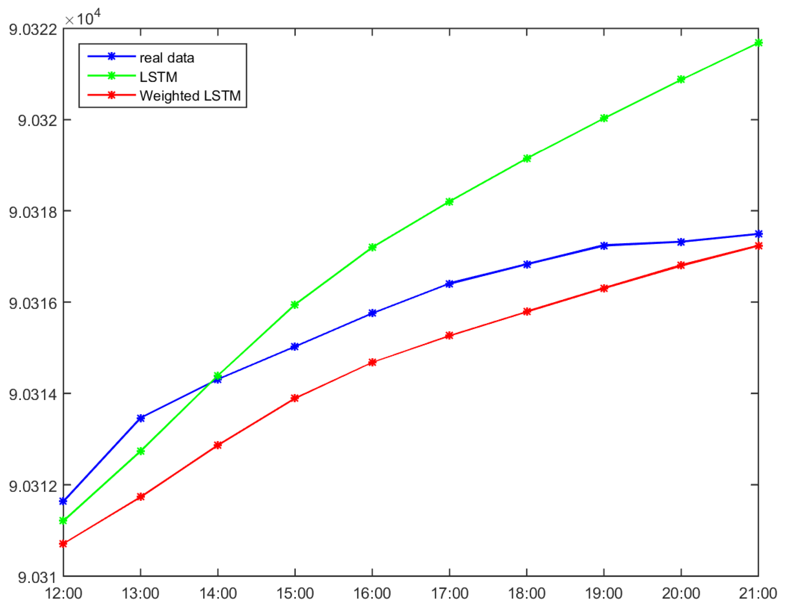
Table 11 presents an example of a case where the results estimated via the LSTM estimation-based method for the data between 12:00 and 21:00, which are the missing data intervals, are larger than the 22:00 data, which appear first after the end of the missing data interval. In fact, 303 customers exhibited such cases in the flipped accumulated usages. The performance of the LSTM estimation-based compensation method may be optimal for some, but it cannot be applied when the case of flipped accumulated usages occurs, as it will trigger a critical error where a negative value of power usage occurs. The real data at 22:00, which appeared first after the end of the missing data interval, was 90,317.66; however, there was an issue, as the 17:00 data produced by the LSTM estimation-based compensation methods was 90,318.2029, which is larger.
Figure 18 presents errors starting from 14:00; according to Figure 18, the data produced by the LSTM estimation-based compensation method are larger than the real data. However, in the LSTM estimate and weight-applied compensation method, the results obtained are never larger than the real data, and the error approaches zero at the ending time of the missing data interval.

4. Conclusions

In this study, we proposed a hybrid algorithm that combines the advantages of the LSTM estimation and linear interpolation methods to correct missing power consumption data. Furthermore, four algorithms of the linear interpolation, past-similar-situation substitution, ARIMA estimation-based compensation, and LSTM estimation-based compensation methods were applied to perform a comparative analysis. For the experiments, we adopted 2-month power usage data by randomly selecting the home usage data of 720 customers that exhibited the most common power consumption patterns. Furthermore, we conducted experiments on missing data by arbitrarily discarding data from the original data that had no missing value. In the experiments, we assumed that 10-h data were missing on a specific day. In the experimental results, the linear interpolation and LSTM estimation-based compensation methods exhibited the best performances among the four algorithms. The linear interpolation method exhibited the same usage for each time band, which did not represent the actual power consumption pattern. The LSTM estimation-based compensation method best represented the power consumption pattern; however, sometimes, its results were larger than the accumulated usage in the first data appearing after the end of the missing data interval (flipped phenomenon). When the weight was applied to the LSTM estimation, i.e., when the method proposed in this study was applied, the 10-h total of the average MAE for all customers was 2.1545, exhibiting the best result. Furthermore, the proposed method did not exhibit the flipped phenomenon, which was the disadvantage of the LSTM estimation; it exhibited the highest stability and performance, rather than the identical usage patterns of the linear interpolation method. There are several important implications presented by the experimental results. First, in general, the linear interpolation method exhibits better performance while being simple, compared to several methods that provide optimal results in the time-series field. If the number of data in the missing value interval is small, it will be the fastest and most effective. Second, if the future values are predicted, rather than estimating the missing data in the middle, the LSTM estimation-based compensation method will be effective. Third, the accumulated value in the power usage data increases continuously. Therefore, if it is corrected by estimating the interval usage in the missing data, the interval usage at the pertinent hour is added to the accumulated usage value, and the error increases gradually as more missing data are increasingly corrected. Therefore, an error may occur, such that the result is larger than the accumulated usage of the first data appearing after the end of the missing data interval. The implications of the experimental results of this study are not only valid for electric energy, as they will be equally effectively beneficial in the demand/supply of other energy sources. Furthermore, the results presented in this study imply that for systems that provide services by collecting meter reading data, it would be effective to construct a system that combines several methods. Based on the knowledge and experience gained in this research, we will conduct a study in the future to apply a missing data-processing algorithm to a system that collects meter reading data.

Author Contributions

Methodology, H.-R.K.; software, H.-R.K.; validation, H.-R.K.; formal analysis, H.-R.K.; writing—original draft preparation, H.-R.K. and P.-K.K.; writing—review and editing, H.-R.K. and P.-K.K.; supervision, P.-K.K.; project administration, P.-K.K. All authors have read and agreed to the published version of the manuscript.

Funding

This work was supported by the National Research Foundation of Korea(NRF) grant funded by the Korea government(MSIT) (No. NRF-2020R1A2C2007091).

Conflicts of Interest

The funders had no role in the design of the study; in the collection, analyses, or interpretation of data; in the writing of the manuscript, or in the decision to publish the results.

References

  1. Jung, J.; Seo, C. An Efficient Method for Meter Data Collection in AMI System. J. Korean Inst. Commun. Inf. Sci. 2018, 43, 1311–1320. [Google Scholar]
  2. Dusa, P.; Novac, C.; Purice, E.; Dodun, O.; Slătineanu, L. Configuration a Meter Data Management System using Axiomatic Design. Procedia CIRP 2015, 34, 174–179. [Google Scholar] [CrossRef] [Green Version]
  3. Kang, H.-J. A Study on the AMI Communication Method Combining High-Rate PLC of ISO/IEC 12139-1 and IEEE 802.15.4g Based Wi-SUN. Ph.D. Dissertation, Department of Electronic Communication Engineering Graduate School Chonnam National University. Gwangju, Korea, 2018. [Google Scholar]
  4. Kwon, H.R.; Hong, T.E.; Kim, P.K. Estimate method of missing data using Similarity in AMI system. Smart Media J. 2019, 8, 80–84. [Google Scholar] [CrossRef]
  5. Qian, X.; Yang, Y.; Li, C.; Tan, S.C. Economic Dispatch of DC Microgrids Under Real-Time Pricing Using Adaptive Differential Evolution Algorithm. In Proceedings of the 2020 IEEE 9th International Power Electronics and Motion Control Conference (IPEMC2020-ECCE Asia), Nanjing, China, 29 November–2 December 2020. [Google Scholar]
  6. Song, H.; Yoon, Y.; Kwon, S. Optimal scheduling of critical peak pricing considering photovoltaic generation and electric vehicle load. In Proceedings of the 2019 IEEE Transportation Electrification Conference and Expo, Asia-Pacific (ITEC Asia-Pacific), Seogwipo, Korea, 8–10 May 2019. [Google Scholar]
  7. Lv, H.; Wang, Y.; Dong, X.; Jiang, F.; Wang, C.; Zhang, Z. Optimization Scheduling of Integrated Energy System Considering Demand Response and Coupling Degree. In Proceedings of the 2021 IEEE/IAS 57th Industrial and Commercial Power Systems Technical Conference (I&CPS), Las Vegas, NV, USA, 27–30 April 2021. [Google Scholar]
  8. Choi, M.-S. Development and Performance Analysis of Hybrid Communication Technology for AdvancedMetering Infrastructure System. KIEE 2020, 69, 610–616. [Google Scholar] [CrossRef]
  9. Inga, E.; Hincapié, R.; Céspedes, S. Capacitated Multicommodity Flow Problem for Heterogeneous Smart Electricity Metering Communications Using Column Generation. Energies 2020, 13, 97. [Google Scholar] [CrossRef] [Green Version]
  10. Chen, W.; Zhou, K.; Yang, S.; Wu, C. Data quality of electricity consumption data in a smart grid environment. Renew. Sustain. Energy Rev. 2017, 75, 98–105. [Google Scholar] [CrossRef]
  11. Choi, Y.J.; Kim, S.Y. Analysis on The Change of Power Consumption Pattern According to Single-Households. In Proceedings of the 2014 Conference on The Korean Institute of Electrical Engineers, Jeju, Korea, 15–19 June 2014; pp. 153–154. [Google Scholar]
  12. Lee, J.; Shin, J.; Joo, Y.; Noh, J.; Park, Y.; Jung, N. A VEE Algorithm Improvement Research for Improving Estimation Accuracy and Verification Responsibility of The AMI Meter Data. KEPCO J. Electr. Power Energy 2016, 2, 557–562. [Google Scholar] [CrossRef] [Green Version]
  13. Jang, M.; Nam, K.; Lee, Y. Analysis and Application of Power Consumption Patterns for Changing the Power Consumption Behaviors. J. Korea Inst. Inf. Commun. Eng. 2021, 25, 603–610. [Google Scholar]
  14. Kim, J.-O. A Study on the Prediction of Short Term Electric Power Load by Deep Learning System. Master’s Dissertation, Dankook University, Yongin-si, Korea, 2019. [Google Scholar]
  15. Ryu, S. Deep Learning for Electric Load Data Analytics. Master’s Dissertation, Sogang University, Seoul, Korea, 2020. [Google Scholar]
  16. Choi, H. Short-Term Load Forecasting Based on ResNet and LSTM. Master’s Dissertation, Sogang University, Seoul, Korea, 2018. [Google Scholar]
  17. Kim, D. Short-Term Load Forecasting Based on LSTM and CNN. Master’s Dissertation, Konkuk University, Seoul, Korea, 2019. [Google Scholar]
  18. Kwon, B.-S.; Park, R.-J.; Song, K.-B. Analysis of Short-Term Load Forecasting Accuracy Based on Various Normalization Methods. J. Korean Inst. Illum. Electr. Install. Eng. 2018, 32, 30–33. [Google Scholar]
  19. Koh, S. Outlier Detection and Imputation Method for Smart Meter Data Using Pattern Analysis. Master’s Dissertation, Korea University, Seoul, Korea, 2019. [Google Scholar]
  20. Timofey, S.; Antonio, N. Fraction-of- Time Density Estimation Based on Linear Interpolation of Time Series. In Proceedings of the 2021 Systems of Signals Generating and Processing in the Field of on Board Communications Signals Generating and Processing in the Field of on Board Communications, Moscow, Russia, 16–18 March 2021; pp. 1–4. [Google Scholar]
  21. Seo, S.-W.; Kim, D.-H.; Kim, S.J. A Study on the Linear Compensation Method of Ideal Surface Roughness to Actual Roughness in Milling. Korean Soc. Manuf. Process. Eng. 2016, 15, 15–20. [Google Scholar]
  22. Pejić, N.; Cvetanović, M.; Radivojević, Z. Estimating similarity between differently compiled procedures using neural networks. In Proceedings of the 2019 27th Telecommunications Forum (TELFOR), Serbia, Belgrade, 26–27 November 2019; pp. 26–27. [Google Scholar]
  23. Lee, S. Applying Different Similarity Measures based on Jaccard Index in Collaborative Filtering. J. Korea Soc. Comput. Inf. 2021, 26, 47–53. [Google Scholar]
  24. Behera, A.P.; Gaurisaria, M.K.; Rautaray, S.S.; Pandey, M. Predicting Future Call Volume Using ARIMA Models. In Proceedings of the 2021 5th International Conference on Intelligent Computing and Control Systems (ICICCS) Intelligent Computing and Control Systems (ICICCS), Madurai, India, 6–8 May 2021; pp. 1351–1354. [Google Scholar]
  25. Garlapati, A.; Krishna, D.R.; Garlapati, K.; Rahul, U.; Narayanan, G. Stock Price Prediction Using Facebook Prophet and Arima Models. In Proceedings of the 2021 6th International Conference for Convergence in Technology (I2CT) Convergence in Technology (I2CT), Maharashtra, India, 2–4 April 2021; pp. 1–7. [Google Scholar]
  26. Chang, H.; Park, D.; Lee, Y.; Yoon, B. Multiple time period imputation technique for multiple missing traffic variables: Nonparametric regression approach. Can. J. Civ. Eng. 2012, 39, 448–459. [Google Scholar] [CrossRef]
  27. Asif, M.T.; Mitrovic, N.; Dauwels, J.; Jaillet, P. Matrix and Tensor Based Methods for Missing Data Estimation in Large Traffic Networks. IEEE Trans. Intell. Transp. Syst. 2016, 17, 1816–1825. [Google Scholar] [CrossRef]
  28. Shakir, M.; Marwala, T. Neural network based techniques for estimating missin data in databases. In Proceedings of the 16th Annual Symposium of the Recognition Association of South Africa, Langebaan, South Africa, 23–25 November 2005. [Google Scholar]
  29. Kwon, H.R.; Hong, T.E. Method of estimation of missing data in AMI system. In Proceedings of the 9th International Conference on Smart Media & Applications, Jeju Island, Korea, 17–19 September 2020. Paper ID-8. [Google Scholar]
  30. Huang, Z.; Zhu, T. Real-time data and energy management in microgrids. In Proceedings of the 2016 IEEE Real-Time Systems Symposium (RTSS), Porto, Portugal, 29 November–22 December 2016; pp. 79–88. [Google Scholar]
  31. Peppanen, J.; Zhang, X.; Grijalva, S.; Reno, M.J. Handling bad or missing smart meter data through advanced data imputation. In Proceedings of the 2016 IEEE Power &Energy Society, Innovative Smart Grid Technologies Conference (ISGT), Minneapolis, MN, USA, 6–9 September 2016; pp. 1–5. [Google Scholar]
  32. Yu, K.; Guo, G.-D.; Li, J.; Lin, S. Quantum Algorithms for Similarity Measurement Based on Euclidean Distance. Int. J. Theor. Phys. 2020, 59, 3134–3144. [Google Scholar] [CrossRef]
  33. Iglesias, F.; Kastner, W. Analysis of Similarity Measures in Times Series Clustering for the Discovery of Building Energy Patterns. Energies 2013, 2013, 579–597. [Google Scholar] [CrossRef] [Green Version]
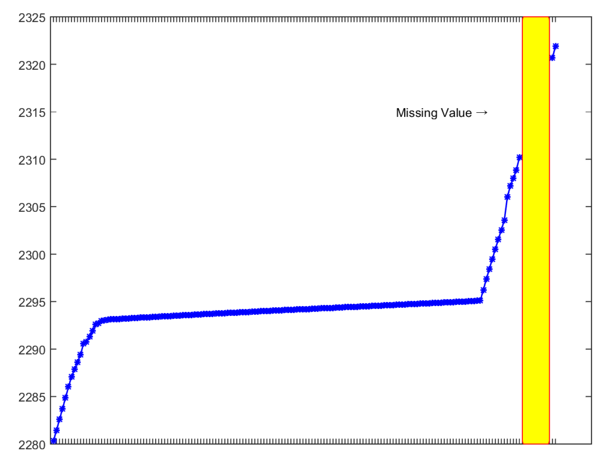
Figure 1. Example of electricity consumption data with missing values.
Information 12 00341 g001
Figure 2. Calculation method of linear interpolation.
Information 12 00341 g002
Figure 3. Similar-past-situation substitution.
Information 12 00341 g003
Figure 4. Power consumption data: abnormal data (non-stationary).
Information 12 00341 g004
Figure 5. Comparison of linear interpolation results and real data.
Information 12 00341 g005
Figure 6. Comparison between the real data and the results obtained from the past-similar-situation substitution method.
Information 12 00341 g006
Figure 7. ACF (Autocorrelation Function).
Information 12 00341 g007
Figure 8. PACF (Partial Autocorrelation Function).
Information 12 00341 g008
Figure 9. Comparison between the real data and ARIMA-based compensation results.
Information 12 00341 g009
Figure 10. Example of comparison between the LSTM estimation results and real data.
Information 12 00341 g010
Figure 11. Comparison between the real data and results of the LSTM estimation-based compensation method.
Information 12 00341 g011
Figure 12. Concept of missing data intervals.
Information 12 00341 g012
Figure 13. Comparison between the real data and the results obtained from the LSTM estimate and weight-applied compensation method.
Information 12 00341 g013
Figure 14. MAE of the four methods for all customers.
Information 12 00341 g014
Figure 15. MAE of the five methods for all customers.
Information 12 00341 g015
Figure 16. Comparison of errors between the LSTM estimate and weight-applied compensation method and the linear interpolation method.
Information 12 00341 g016
Figure 17. Comparison of errors between the LSTM estimate and weight-applied compensation method and the LSTM estimation-based compensation method.
Information 12 00341 g017
Figure 18. Comparison among the LSTM estimate and weight-applied compensation, LSTM estimation-based compensation, and real data.
Information 12 00341 g018
Table 1. AMI supply forecast (existing) and performance (Unit: 10,000, cumulative).
Year201520162017201820192020
Outlook73010001250150018302250
Performance250435520680980-
Press release from the Ministry of Trade, Industry, and Energy (18 July 2018).
Table 2. Data for linear interpolation-based correction.
TimeAccumulated UsageInterval UsageLinear UsageEstimated UsageAbsolute Error
11:002310.191.351---
12:002311.1340.9442311.14220.95220.0082
13:002311.7430.6092312.09440.95220.3514
14:002311.9450.2022313.04650.95221.1015
15:002312.770.8252313.99870.95221.2287
16:002312.9080.1382314.95090.95222.0429
17:002313.0480.142315.90310.95222.8551
18:002313.1410.0932316.85530.95223.7143
19:002313.5470.4062317.80750.95224.2605
20:002317.1013.5542318.75960.95221.6586
21:002318.661.5592319.71180.95221.0518
22:002320.6642.004---
Table 3. Euclidean similarity data.
Time4/174/184/194/204/214/224/234/24
2:001.0481.0951.1390.0190.0190.0180.010.011
3:001.0411.1041.1170.0190.010.0110.0180.017
4:001.0211.0711.1730.0190.0180.0180.0120.018
5:001.0121.0691.140.0190.0180.010.0160.01
6:001.0111.0871.0750.0180.0160.0170.0180.018
7:002.461.9360.7670.0190.0120.0180.010.01
8:001.1530.7480.790.010.0180.010.0180.018
9:000.8370.7370.7620.0180.0140.0180.010.018
10:000.8291.4011.1830.0190.0150.0110.0180.01
11:001.3510.8280.1460.0180.0180.0180.010.018
Sum Of Error-2.4174.20111.58511.60511.61411.62311.615
Table 4. Reference data at the same time band of similar past situations.
YMDTimeAccumulated UsageInterval Usage
4/182:002258.7261.095
4/183:002259.831.104
4/184:002260.9011.071
4/185:002261.971.069
4/186:002263.0571.087
4/187:002264.9931.936
4/188:002265.7410.748
4/189:002266.4780.737
4/1810:002267.8791.401
4/1811:002268.7070.828
4/1812:002269.2950.588
4/1813:002269.3490.054
4/1814:002269.3920.043
4/1815:002269.4550.063
4/1816:002269.630.175
4/1817:002269.8580.228
4/1818:002270.3080.45
4/1819:002270.980.672
4/1820:002272.9952.015
4/1821:002275.5342.539
Table 5. Compensation data based on the past-similar-situation substitution method.
TimeAccumulated UsageInterval UsageSimilar EstimatedSimilar IntervalAbsolute Error
12:002311.1340.9442310.7780.5880.356
13:002311.7430.6092310.8320.0540.911
14:002311.9450.2022310.8750.0431.07
15:002312.770.8252310.9380.0631.832
16:002312.9080.1382311.1130.1751.795
17:002313.0480.142311.3410.2281.707
18:002313.1410.0932311.7910.451.35
19:002313.5470.4062312.4630.6721.084
20:002317.1013.5542314.4782.0152.623
21:002318.661.5592317.0172.5391.643
Table 6. Data corrected via the ARIMA-based compensation method.
TimeAccumulated UsageInterval UsageARIMA EstimatedARIMA IntervalAbsolute Error
12:002311.1340.9442311.28770.15370.1537
13:002311.7430.6092312.33280.58980.5898
14:002311.9450.2022313.28511.34011.3401
15:002312.770.8252314.16311.39311.3931
16:002312.9080.1382314.96992.06192.0619
17:002313.0480.142315.71212.66412.6641
18:002313.1410.0932316.39463.25363.2536
19:002313.5470.4062317.02233.47533.4753
20:002317.1013.5542317.59950.49850.4985
21:002318.661.5592318.13030.52970.5297
Table 7. Experimental environment.
DeviceModelSpec
OSWindows 10 64 bit-
CPUIntel(R) Core(TM)[email protected] GHz-
MEM-8 GB
GPUIntel(R) UHD Graphics 620-
Table 8. Data corrected based on the LSTM estimation.
TimeAccumulated UsageInterval UsageLSTM EstimatedLSTM IntervalAbsolute Error
12:002311.1340.9442311.2190.0850.085
13:002311.7430.6092312.37470.63170.6317
14:002311.9450.2022313.36281.41781.4178
15:002312.770.8252313.97711.20711.2071
16:002312.9080.1382314.43051.52251.5225
17:002313.0480.142314.88461.83661.8366
18:002313.1410.0932315.29462.15362.1536
19:002313.5470.4062315.61482.06782.0678
20:002317.1013.5542316.0481.0531.053
21:002318.661.5592317.12431.53571.5357
Table 9. Data corrected by applying the LSTM estimates and weights.
TimeAccumulated UsageLSTM EstimatedLSTM TermRateW.LSTM UsageW.LSTM EstimatedAbsolute Error
11:002310.19-----
12:002311.1340.89430.10791.12992311.31990.1859
13:002311.7431.00490.12121.26972312.58960.8466
14:002311.9450.90780.10951.1472313.73651.7915
15:002312.770.55460.06690.70072314.43721.6672
16:002312.9080.49060.05920.61992315.05712.1491
17:002313.0480.29050.0350.3672315.42412.3761
18:002313.1410.29250.03530.36962315.79372.6527
19:002313.5470.36970.04460.46712316.26082.7138
20:002317.1010.49060.05920.61992316.88070.2203
21:002318.661.15360.13921.45752318.33820.3218
22:002320.6641.84080.22212.32582320.6640
Table 10. Mean absolute error (MAE) for all customers.
TimeLinearSimilarARIMALSTMWeight LSTM
12:000.09320.09760.07810.0880.105
13:000.15780.17630.16410.15340.1751
14:000.2130.24590.25270.20330.2208
15:000.25780.3160.3430.24220.2494
16:000.28970.38770.43530.27630.2779
17:000.31120.46850.54310.3130.292
18:000.31380.54460.6730.35970.2867
19:000.27810.62270.82970.41240.2524
20:000.20420.68690.99710.45970.1877
21:000.11210.74371.18330.50360.1075
SUM2.23094.28995.49943.01162.1545
Table 11. Example of errors in data corrected using the LSTM estimation.
YMDTimeAccumulated UsageLSTM EstimatedWeight LSTM
4/2512:0090,311.6490,311.21390,310.7109
4/2513:0090,313.4690,312.731590,311.7347
4/2514:0090,314.3190,314.393290,312.8699
4/2515:0090,315.0290,315.947890,313.8991
4/2516:0090,315.7690,317.201590,314.6807
4/2517:0090,316.4190,318.202990,315.266
4/2518:0090,316.8390,319.146690,315.7897
4/2519:0090,317.2490,320.028390,316.3056
4/2520:0090,317.3290,320.872790,316.8031
4/2521:0090,317.4990,321.676590,317.2351
Publisher’s Note: MDPI stays neutral with regard to jurisdictional claims in published maps and institutional affiliations.