Article

Autoencoder Based Analysis of RF Parameters in the Fermilab Low Energy Linac

by
Jonathan P. Edelen
*,† and
Christopher C. Hall
RadiaSoft LLC, Boulder, CO 80301, USA
*
Author to whom correspondence should be addressed.
Current address: 6525 Gunpark Dr., Suites 370-411, Boulder, CO 80301, USA.
Information 2021, 12(6), 238; https://doi.org/10.3390/info12060238
Submission received: 28 March 2021 / Revised: 25 May 2021 / Accepted: 26 May 2021 / Published: 31 May 2021
(This article belongs to the Special Issue Machine Learning and Accelerator Technology)

Abstract

:
Machine learning (ML) has the potential for significant impact on the modeling, operation, and control of particle accelerators due to its ability to model nonlinear behavior, interpolate on complicated surfaces, and adapt to system changes over time. Anomaly detection in particular has been highlighted as an area where ML can significantly impact the operation of accelerators. These algorithms work by identifying subtle behaviors of key variables prior to negative events. Efforts to apply ML to anomaly detection have largely focused on subsystems such as RF cavities, superconducting magnets, and losses in rings. However, dedicated efforts to understand how to apply ML for anomaly detection in linear accelerators have been limited. In this paper the use of autoencoders is explored to identify anomalous behavior in measured data from the Fermilab low-energy linear accelerator.

1. Introduction

In recent years machine learning (ML) has been identified as having the potential for significant impact on the modeling, operation, and control of particle accelerators [1,2]. These techniques are attractive due to their ability to model nonlinear behavior, interpolate on complicated surfaces, and adapt to system changes over time.
Neural networks have been applied to accelerator diagnostics to provide predictions for destructive diagnostics when the diagnostic is not inserted into the beam-line [3,4]. Neural networks have also been used for a range of machine tuning problems through the generation of inverse models [5,6]. When combined with optimization algorithms, these inverse models have demonstrated improved switching times between operational configurations in free-electron lasers [7]. Significant speed up has been demonstrated in multi-objective optimization of accelerators by using neural networks as surrogate models [8].
Anomaly detection has been highlighted as an area where ML can significantly impact the operation of accelerators. Recent efforts have been aimed at understanding and predicting faulty behavior in superconducting RF cavities [9,10,11] and magnets [12]. This is of interest due to the potentially catastrophic nature of a failure in these devices. Additionally, ML has been used to identify and remove malfunctioning beam position monitors in the LHC, prior to application of standard optics correction algorithms [13]. Other efforts have sought to use ML for detection of errors in hardware installation [14]. More broadly, machine learning for anomaly detection has been an active area of research for some time; including the development of new frameworks for isolating anomalies in IoT scenarios [15] and in wireless networks [16].
While many of these efforts have shown success, results of more global fault prediction have been limited. A recent effort at J-PARC utilized the System Invariant Analysis Technique to develop an operational fault prediction algorithm [17], however, results are still preliminary and there is significant room for development in this area especially loss classification and fault prediction. Loss prediction has been studied at the LHC [18], but efforts to use ML for loss classification in linear accelerators (linacs) have been limited. Understanding loss mechanisms in linacs can be challenging as they often have limited diagnostics. Thus, the relationship between tunable parameters and the beam transmission can be difficult to untangle. Moreover, because the primary function of linacs is to deliver as much current as possible to the subsequent acceleration stages, understanding the root cause of performance degradations is critical to the experimental program of any accelerator facility.
In this work autoencoders are used to better correlate changes in the RF cavities to the changes in the transmission at the low energy proton linac at Fermi National Laboratory (Fermilab). Our methodology is to train autoencoders on measurements of the amplitude and phase signals in the RF cavities and correlate the output of the autoencoder with changes in the amount of beam current transmitted by the linac. In the first section a brief overview of autoencoders, followed by some background on the linac is given. Results of principal component analysis, using an autoencoder, are shown and then compared with traditional methods in the second section. Finally, the quantification of anomalous machine states is demonstrated using the autoencoder reconstruction error. In each case the autoencoder analysis displays a larger correlation between the beam current of the linac and the amplitude and phase signals in the cavities than is evident by conventional analysis. This result indicates that changes in the beam current can be attributed to a change in state of the corresponding RF cavities.

2. Materials and Methods
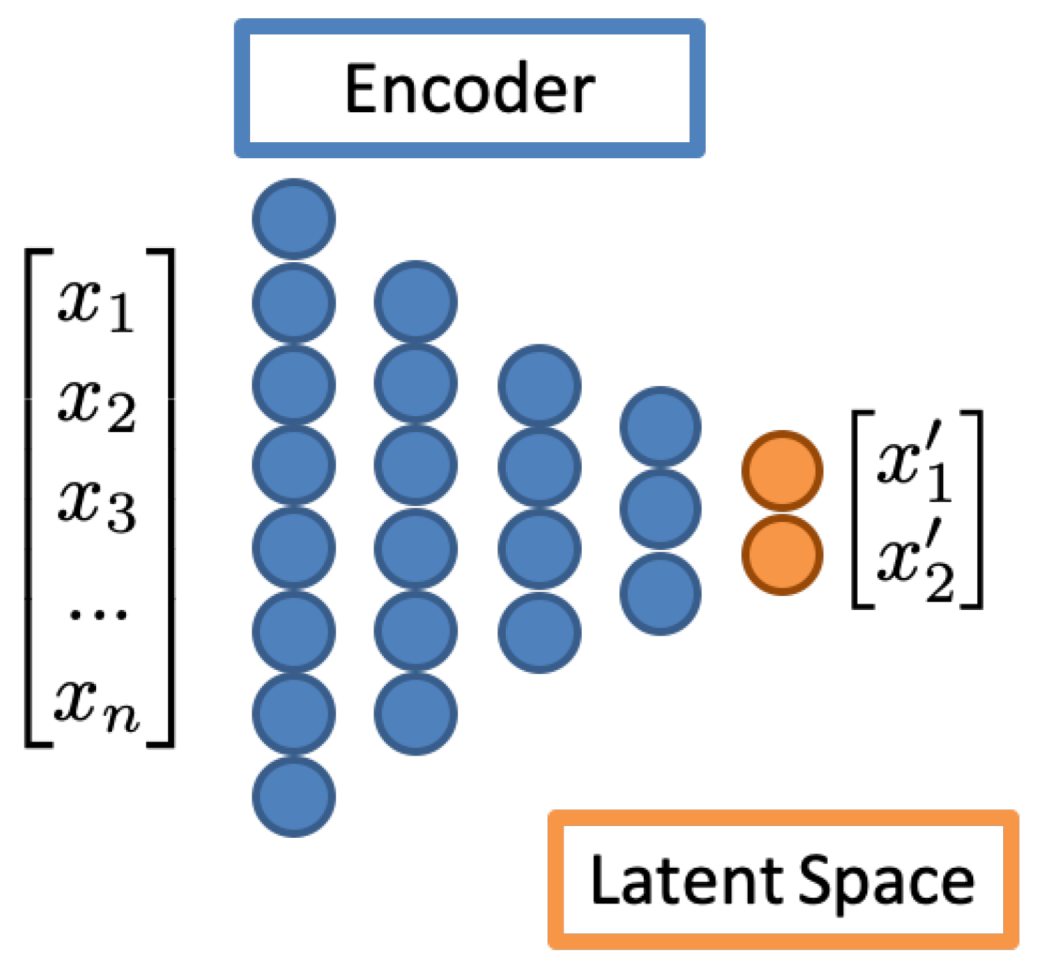
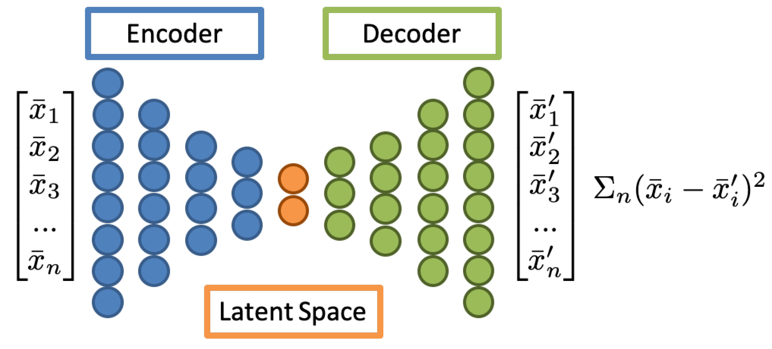
2.1. Autoencoders

Autoencoders are a class of neural networks that effectively learn an identity transformation on a specified dataset while subsequently reducing its dimensionally. A schematic of an autoencoder is shown in Figure 1. Here the number of nodes is steadily decreased in the encoder section (Blue). The encoded dimension (Orange), also referred to as the latent space, is the minimum number of nodes. The number of nodes per layer then increases in the decoder section (Green) to reproduce the input data. The base dimensionality of the dataset is determined by the number of nodes at the encoded dimension. Typically the encode and decode sections of the network are symmetric.
Autoencoders are commonly used in two configurations. One configuration is the direct analysis of the latent space. This is accomplished by removing the decoder section from the network and analyzing the output of the latent space nodes directly, as shown in Figure 2.
The second configuration, shown in Figure 3, is used to quantify the relationship between a training dataset and a test dataset. Here one evaluates the ability for the autoencoder to reconstruct a given input data set.
While autoencoders have fairly broad applicability in ML, here they are employed for nonlinear principal component analysis (PCA) [19], or for reconstruction analysis. Due to the transformation being inherently nonlinear, the information encoded in the reduced dimensionality space may contain more information, as compared with traditional PCA methods. Additionally, when anomalous behavior is not well understood or not well sampled, an autoencoder can be trained on so-called “good data”. The ability of the autoencoder to reconstruct new data provides a quantitative metric for how similar the new data are to the “good data”. In this work both latent space analysis and reconstruction error—for identifying fundamental changes—were explored in data taken from diagnostics in the Fermilab linac. It is shown that autoencoders could capture relationships that were not easily detectable with other, more traditional, methods.

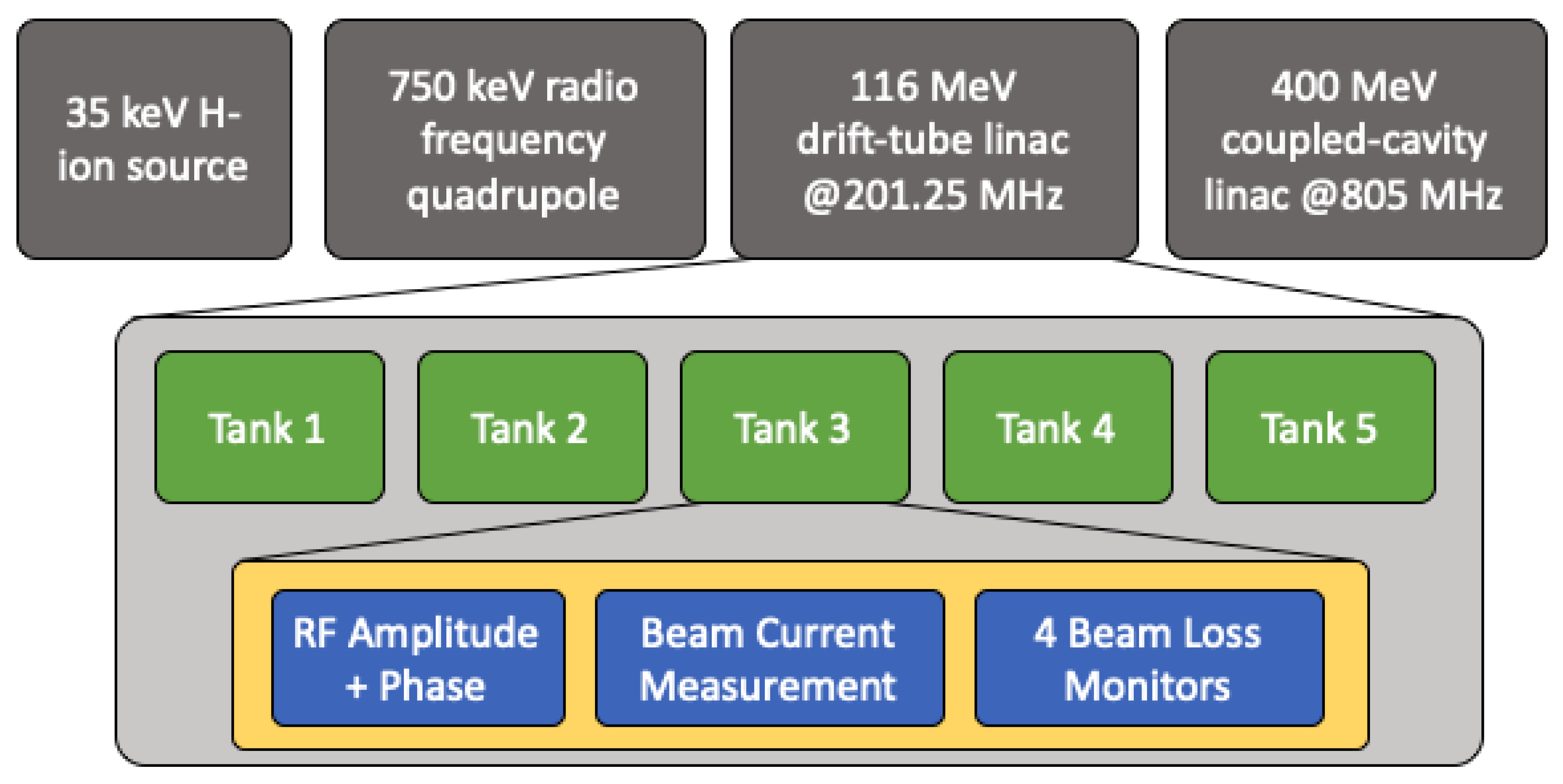
2.2. Overview of the Fermilab Linac

The Fermilab linac accelerates H ions from the 35 keV ion source to 400 MeV for injection into the Booster Synchrotron. From the Booster ions are stripped of their electrons and accelerated to 8 GeV for use in experiments or accelerated further for high-energy experiments. The linac consists of three accelerator sections. First, a Radio Frequency Quadrupole (RFQ) transforms the pulsed DC beam generated in the ion source into a bunched beam while accelerating it to 750 keV. The so-called low-energy linac is an Alvarez style Drift Tube linac (DTL) which consists of five accelerating tanks. Each tank receives RF power from its own klystron which operate at 201.25   M Hz . This portion of the accelerator brings the beam to 116 MeV. The high-energy linac consists of 805 M Hz coupled cavity accelerating structures and brings the beam to the final energy of 400 MeV. For the studies in this paper we are primarily concerned with the performance of the low-energy DTL sections. A schematic of the linac with the associated diagnostics available in the DTL section is shown in Figure 4.
The studies performed here utilized the diagnostic data available for the five DTL sections. For each tank in the DTL RF amplitude and phase measurements were collated from the control system, along with toroid measurements at the exit of each of the DTL tanks. Here the term toroid refers to toroids in DC current transformers [20] used for taking non-destructive measurement of the beam current. The RF control system was responsible for generating a low level signal that was subsequently amplified and used to power the DTL tanks [21]. Pickups inside the DTL tanks were used to measure the amplitude and phase of RF power in each cavity. These signals were digitized and sent back to the control system where they were logged for further analysis. These data were logged over a 22 week period ranging from October 2019 to February 2020 at 15 s intervals. Figure 5 shows the raw RF amplitude and phase as a function of time during the whole operational period. Figure 6 highlights the period of interest starting at week 5.
Figure 7 shows the toroid measurements at the exit of the DTL tanks over the whole 20 week period.
It is clear from the toroid measurements that there was an abrupt change in the machine state at week 13. A cursory analysis of the RF amplitude and phase signals indicates that this was likely a result of changes in the RF parameters, however, a direct comparison was difficult to make.

3. Results

The use of autoencoders was broken down into two primary areas of inquiry, dimensionality reduction and reconstruction testing. For dimensionality reduction an autoencoder was trained on all amplitude and phase measurements during the 22 week period. Once trained output from the latent space of the autoencoder was compared against the toroid current measurements collected during that same period. As a baseline for comparison two other dimensionality reduction methods, singular value decomposition and vector sum analysis, were also applied to the data and shown here. For the reconstruction analysis portion, autoencoders were trained on amplitude and phase measurements taken from just a portion 22 week data period. The trained autoencoders were then used on measurements during the final weeks of the run. The reconstruction error was then correlated with the toroid current measurements during those same time periods.

3.1. Dimensionality Reduction

3.1.1. Conventional Approaches

Before developing the latent space analysis the amplitude and phase signals were studied using vector sum and singular value decomposition (SVD) analyses. These conventional approaches serve as a benchmark for the ML based approach and highlight the advantage of an autoencoder based principal component analysis (PCA) technique. Figure 8 shows the fractional change in the vector sum of the amplitude and phase measurements as a function of time between weeks 5 and 20. Here the data from each of the linac tanks are decomposed into their respective in-phase and quadrature components and then added together for a net in-phase and quadrature signal.
Figure 8 shows that the variation in these signals between the beginning and end of the study period are below 1%.
A running SVD was also performed on the amplitude and phase signals. The SVD was computed in increments of 10 time samples along the period of interest. Because the resulting singular values ranged widely in magnitude, they were scaled using a robust scaler technique. The robust scaler removed the median and scaled the data according to the interquartile range. Centering and scaling happened independently on each feature by computing the relevant statistics on the samples in the data set. This ensured large changes in small singular values would not be washed out by the small changes in large singular values when aggregating. The scaled singular values were added and plotted as a function of time, Figure 9.
Here the change in state of the RF cavities was even less clear than for the vector sum. The quadrature component of the vector sum was suggestive of RF being the reason for the change in beam current, however, the changes were small enough that the relationship was unclear.

3.1.2. Latent Space Analysis

For the latent space analysis, the autoencoders were trained on the amplitude and phase data from all five linac tanks. Prior to training the same robust scaler technique as before was used. Once scaled, the time series data are split into disjoint training and validation sets. Approximately 140 × 103 samples were used for training with approximately 60 × 103 for validation. The batch size was 20 × 103 which yielded seven batches per epoch. When training the networks an epoch was an iteration of the optimizer. Training was run on one batch at a time. Therefore at any given time the weights were only updated using the data in the batch. During each epoch the training iterated over all seven batches. The autoencoders were constructed using Keras [22] and rectified linear units were used as the activation functions. For regularization 30% Gaussian noise was applied at each layer.
Different architectures using one, two, and three principal components were compared, iterating over 10 trials for each.
Figure 10 shows the loss as a function of epoch for the training and validation sets for the three different architectures. These results were averaged over the 10 trials.
From Figure 10 it is clear that more than one encoded dimension was required to represent our dataset. The increase from two to three encoded nodes, however, showed comparatively small improvements. For simplicity when comparing the results with other methods two encoded nodes were used for the remainder of the analysis. Figure 11, shows the fractional change in the encoded dimension as a function of time between weeks 5 and 20. The fractional change was computed relative to the median value of each encoded dimension.
There was a discrete change in the encoded dimensions for both studies around week 12.5. This aligned with the discrete change in the beam current seen in Figure 7. As the amplitudes and phases are being changed leading up to week 18, the principal components continued to vary in a way that was somewhat correlated with the changes seen in Figure 6. However, at around week 17.5 the parameters settled on a new value that was significantly different from the initial values. A direct comparison between the latent space analysis and the vector sum analysis is shown in Figure 12. Here, a rolling average and standard deviation of 100 points was computed for the normalized latent space parameters and the normalized vector sum components.
The latent space parameters varied lightly between weeks 5 and 11 at which point there was an abrupt change. At the end of the operational period, from week 17.5 and on, the latent space settled to a new state that changed by 50% from the period covering weeks 12.5 through 17.5. The change in the vector sum for the same operational period was less than 1%. For copper RF structures such as the one studied in this paper, a change in the vector sum of less than 1% would not raise concerns for operators or experts. However the large change in the latent space provides experts and operators alike with an improved diagnostic about the combined health of the linac section.

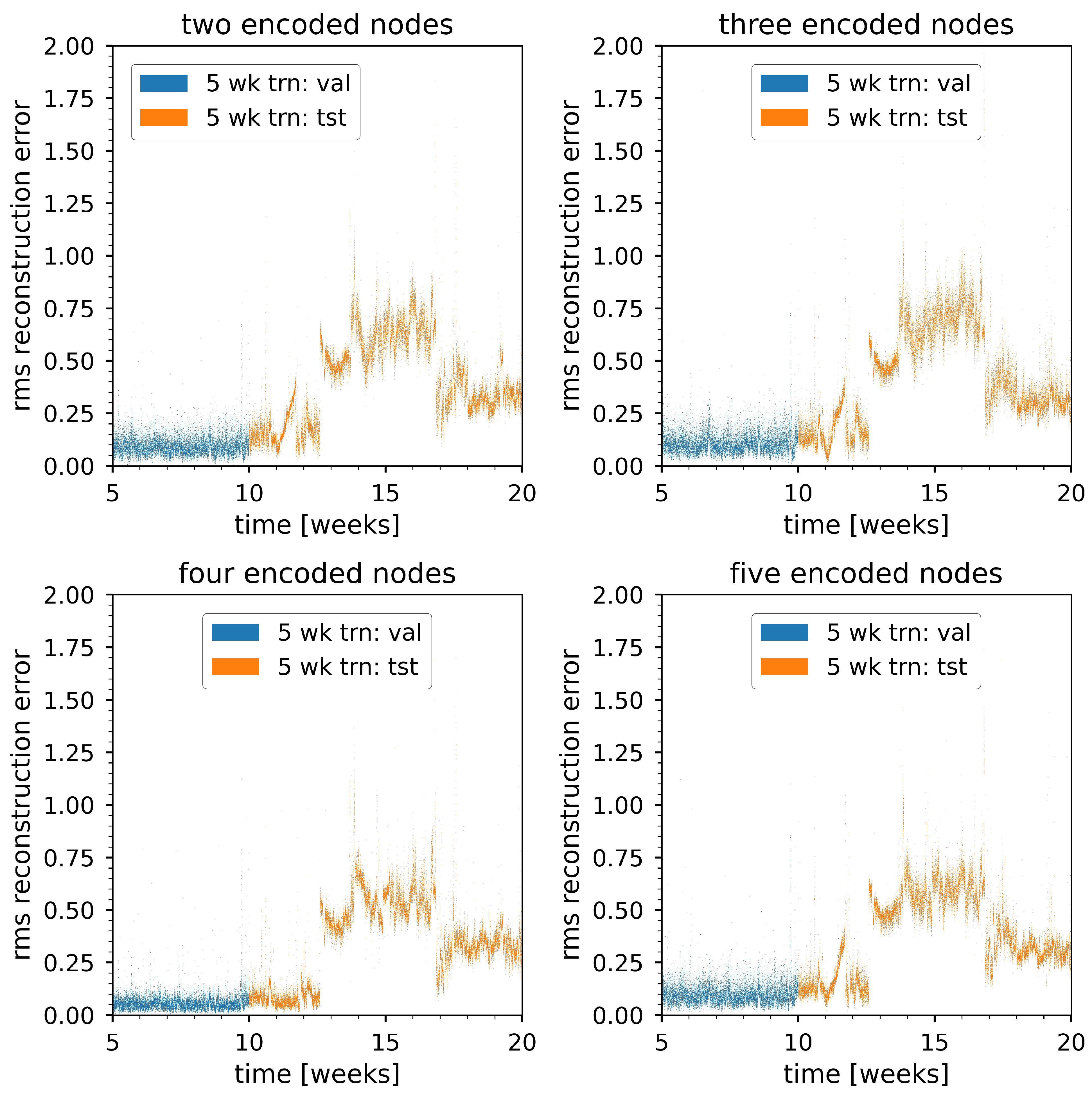
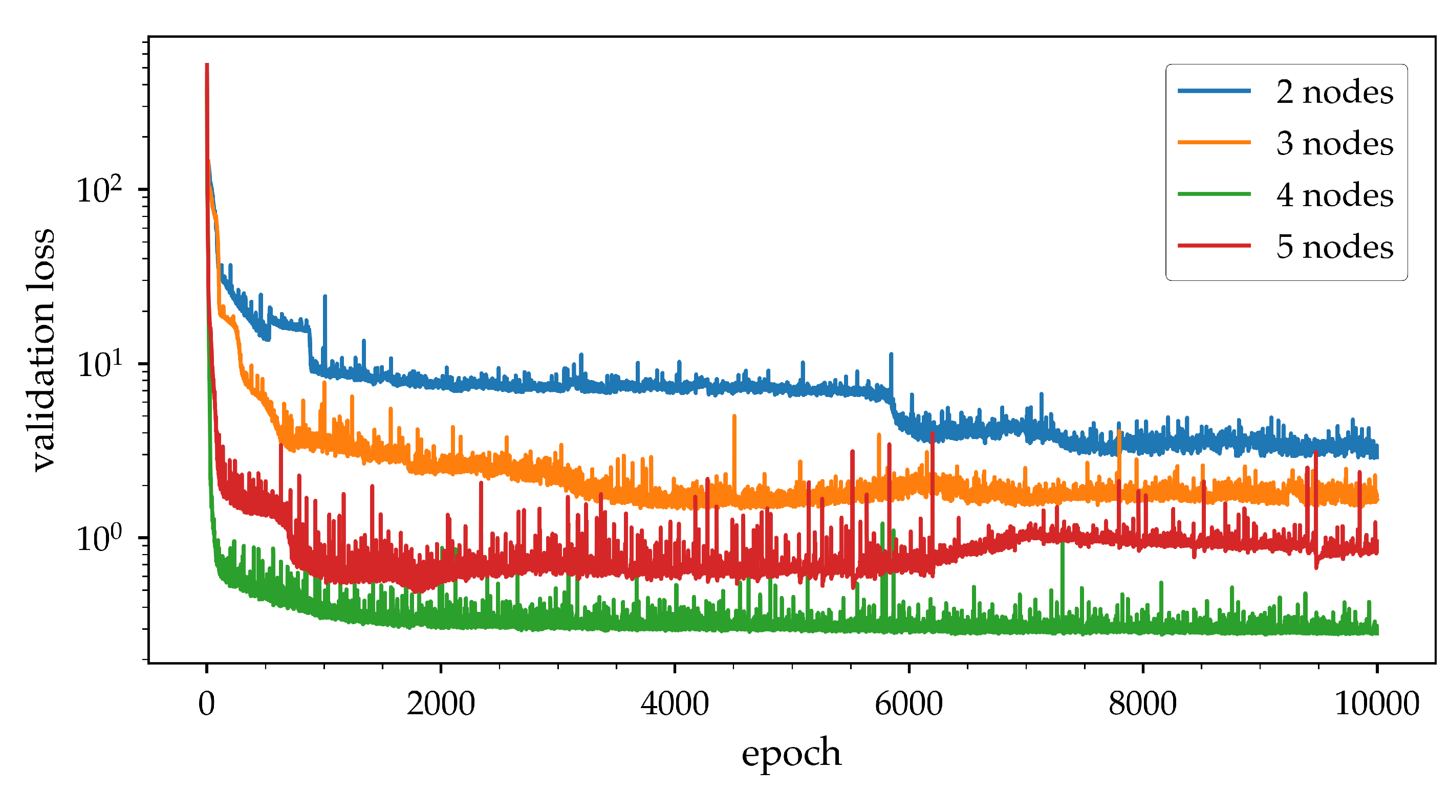
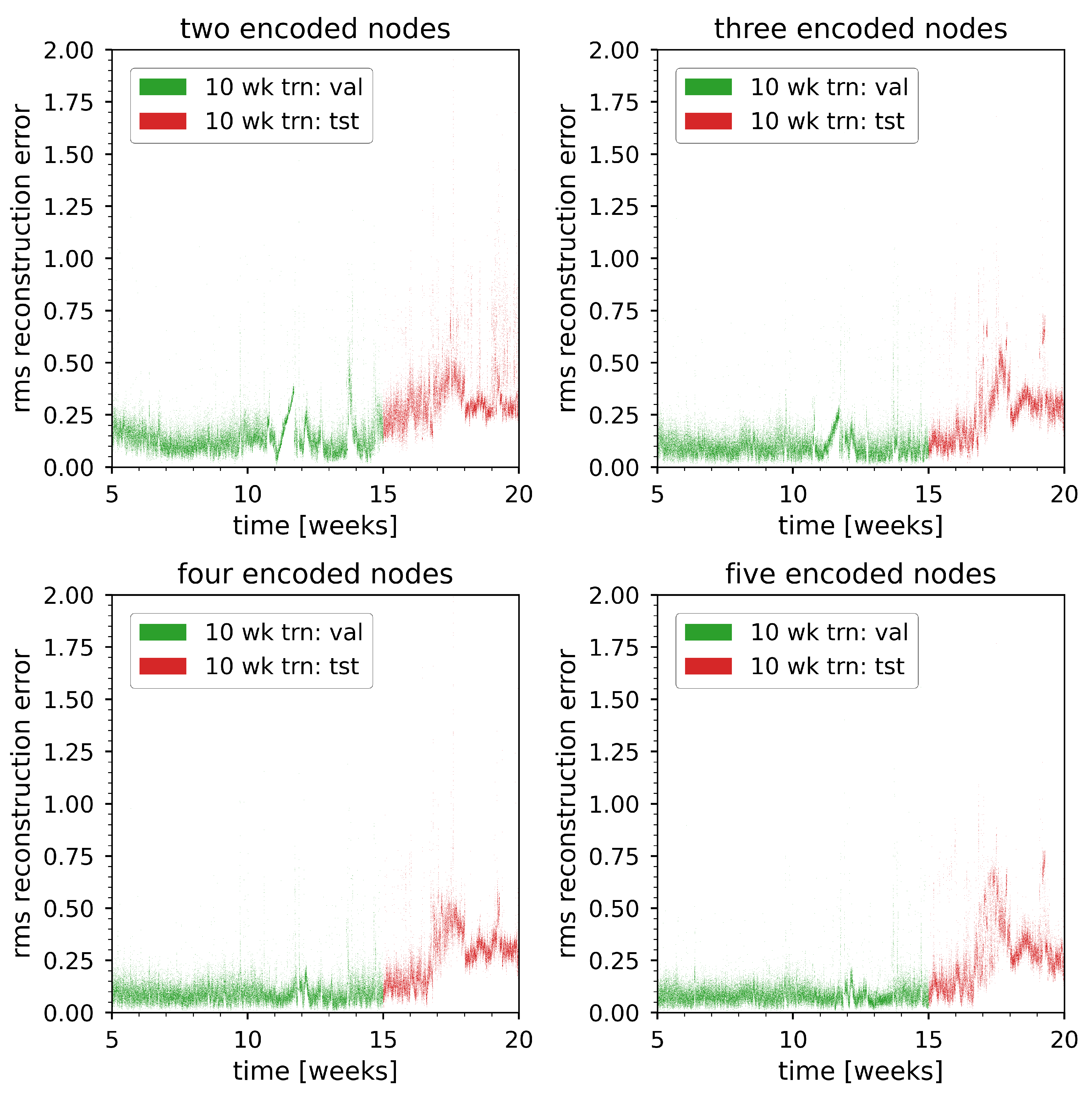
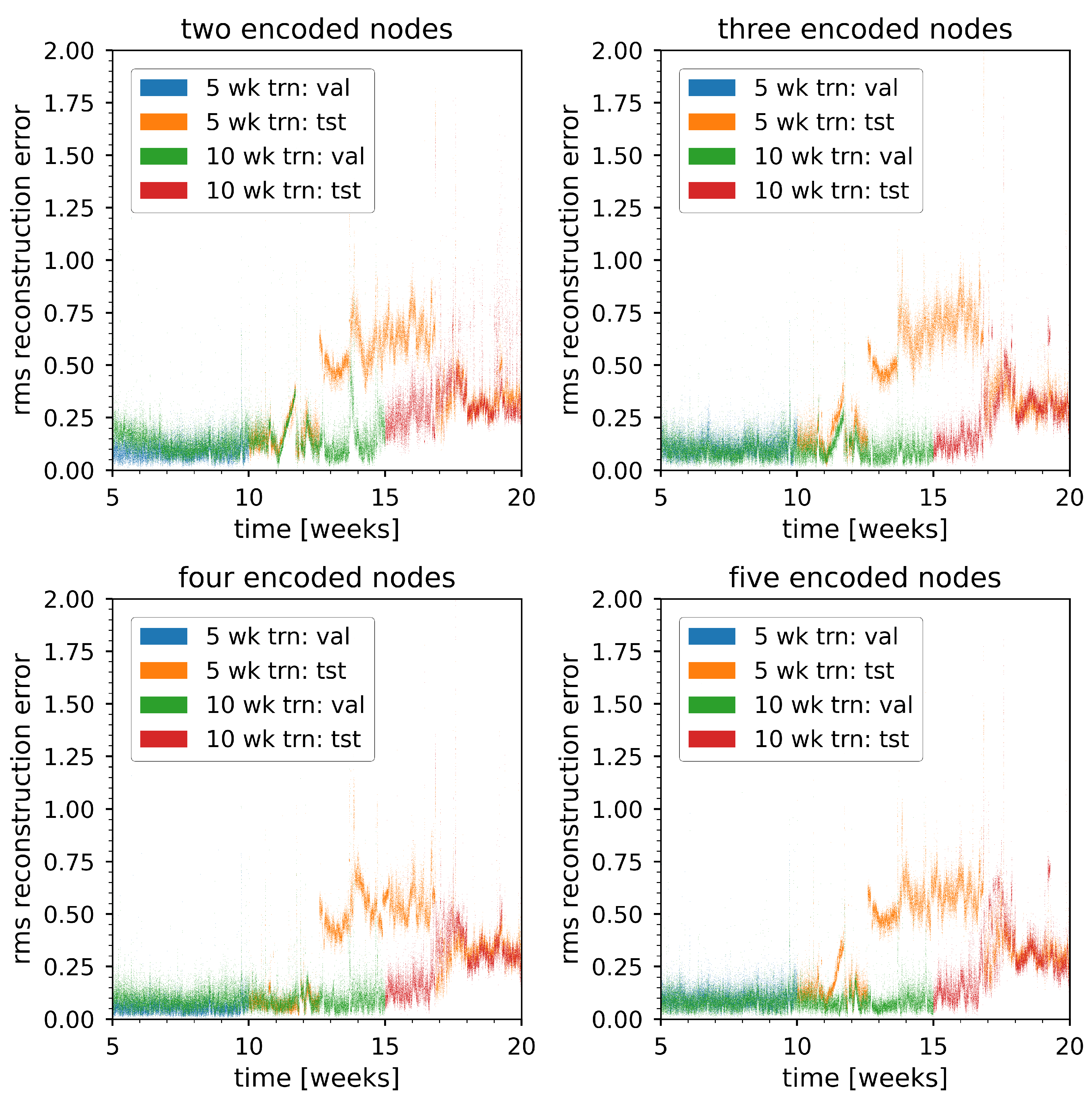
3.2. Reconstruction Analysis

Here autoencoders were used to quantify the similarity of amplitude and phase measurements taken during two different periods of linac operation. This simulatedd a scenerio where an autoencoder was trained on a period of known good operation and tested on a new operational period. Two cases were considered: in the first case training and validation data were taken only from weeks 5 to 10, and for the second case data from weeks 5 to 15 were used for training and validation. The first 5 weeks of operation were omitted as the machine was not yet in a stable configuration. For each case autoencoders were trained to compress and reconstruct the amplitude and phase measurements over the given period. The trained autoencoders were then used to process data taken from later during operation. For the first case testing data were taken from weeks 10 to 20. In the second case only data from weeks 15 to 20 were used. The error in the autoencoder reconstruction was then correlated to the observed changes in the beam current of the low energy linac. Different loss functions, network architectures, and activation functions were examined for the autoencoder. The results presented here utilize rectified linear units for the activation function, Gaussian noise layers for regularization, mean squared error for the loss function, and a symmetric network topology that stepped down from 30 nodes to 10 in increments of 10 then a six node layer and a variable encoded dimension depending on the study in question.
Figure 13 shows validation loss for autoencoders trained on data from weeks 5 to 10. While in all cases the loss curves showed a fast convergence, when there were more than two latent space dimensions there was significant variability in the loss with time.
Figure 14 shows the reconstruction error as a function of time for the validation data and the test data. The caption denotes how many weeks were used for training. Blue denotes the validation data and orange indicates the test data. For each case the increase in latent space dimension correlated with a decrease in the local spread of the reconstruction error both within the validation data and within the test data up to four latent space dimensions. With five latent space dimensions the spread increased again. In all cases, there was an abrupt change in the reconstruction error around week 13 and an offset in the reconstruction error from weeks 18 to 20. This offset correlated directly to the decrease in beam current observed in the linac.
Figure 15 shows the validation loss as a function of epoch for the second case where the autoencoder was trained and validated on data from weeks 5 to 15 and tested on the final 5 weeks. Here it is seen that there is a more direct relationship between the number of latent space dimensions and validation loss. As the number of latent space dimensions increased the validation loss improved until there were signs of over fitting with five latent space dimensions.
Figure 16 shows the RMS reconstruction error as a function of time for the second case. Here the validation data are depicted in green and the test data are shown in red. The caption denotes the number of weeks used for training and validation. As with Figure 14 the reconstruction error was low during the training period and the spread in the error decreased as we increased the number of latent space dimensions. After week 15 there was a steady increase in the reconstruction error which stabilized to an offset during weeks 18 to 20.

4. Discussion

When performing a direct analysis of the latent space it was seen that there are very clear indicators of fundamental changes in the amplitudes and phases of the linac section. These changes were not born out in either the vector sum or SVD analyses of the data. The correlation coefficient between the beam current and the latent space parameters was computed and compared with the direct correlation between the RF parameters and the beam current. In this case the latent space was 10% more correlated with the change in current than the raw amplitude and phase measurements. This indicates that the change in cavity amplitude and phase is related to the change in the beam current in a way that is not made obvious through conventional analysis.
This result is further supported by the reconstruction tests. Figure 17 shows an overlay of the results presented in Figure 14 and Figure 16. As expected the reconstruction error diverges in the weeks where one is trained on more data than the other, the two cases converge in week 17 to the same offset that is present from weeks 18 to 20. Not only do both cases have the same steady state value, but the fine structure in the reconstruction error is borne out in both cases.
Furthermore, the correlation coefficient between the beam current and the reconstruction error were computed for each case and showed the same 10% increase in the correlation as compared to the raw correlation between the beam current and the cavity amplitude and phase signals. This result further indicates that there are fundamental differences in the state of the RF cavities between the end of the 20 week period and the beginning of the 20 week period that are not captured by conventional analysis techniques.
Directly comparing the fractional change measurements from the vector sum analysis in Figure 8 and autoencoder latent variables in Figure 11, the latent variable distribution clearly shows a much higher degree of non-stationary behavior as compared to conventional analysis methods. Comparing the shift in average value (see Figure 12) of the signal from the period from around 12.5 to 17 shows that the autoencoder has a 10 fold greater difference in fractional change as compared to the vector sum method.

5. Conclusions

In this paper autoencoders have been used as a means of anomaly detection and root cause analysis in the Fermilab linac. Specifically, the use of autoencoders for latent space analysis and as a tool to measure similarity of machine states were examined. When comparing the autoencoder to a traditional SVD or vector sum based analysis the autoencoder outperformed these tools when it came to discriminating between different machine states. Moreover, a 10% increase in the correlation between the latent space parameters and the beam current supports the claim that a change in the RF system is the cause of the drop in beam current. The RF system of the linac [23,24] relies on reference signals to maintain phase stability between the accelerated proton beam and RF wave in each tank. A sudden jump in the phase of a reference signal could be the cause of this anomaly. A change in the reference signal might not show up in the vector sum signals but would represent a fundamental change in the amplitude and phase measurements that result in lower beam current out of the linac. A new relationship between the phase and amplitude settings as indicated by the latent space analysis suggests the RF parameters are indeed in different configuration.
Furthermore this work demonstrates that the latent space representation of the amplitude and phase signals is inherently more sensitive to changes than conventional aggregation methods. Thus providing operators with a clearer picture of when the machine is operating normally or abnormally. Moreover, the reconstruction analysis shows similar sensitivity and provides a concise picture of when the machine is operating normally versus abnormally. In both the latent space analysis and the reconstruction analysis the sensitivity to a change in state was 10 fold higher than conventional techniques. An autoencoder trained on data collected during normal operations would be a valuable tool for quickly diagnosing if the machine is in a normal state or which subsystems are experiencing anomalies. In the Fermilab linac specifically, one could build autoencoder representations for each of the three primary acceleration stages and evaluate the reconstruction error over time. This reduces the number of observables for healthy operations from dozens to three. This work has demonstrated that autoencoder representations of the machine are superior to traditional dimensionality reduction techniques and can provide operators with a concise picture about the overall health of the machine.

Author Contributions

J.P.E. was the lead on this effort. He curated the data from the Fermilab archiver system, trained the machine learning models, and performed the analysis used to construct this manuscript. C.C.H. provided key support in evaluating the results and providing feedback for the direction of the analysis. All authors have read and agreed to the published version of the manuscript.

Funding

This material is based upon work supported by the U.S. Department of Energy, Office of Science, Office of High Energy Physics under Award Number DE-SC0019979 and Office of Nuclear Physics under Award Number DE-SC0019682.

Institutional Review Board Statement

Not applicable.

Informed Consent Statement

Not applicable.

Data Availability Statement

Not applicable.

Acknowledgments

The authors wish to acknowledge the Fermi Research Alliance for allowing access to the data that was used for our study. We also wish to acknowledge the support of Auralee Edelen at SLAC for discussions of the methods used in this paper and for discussions on related work in the field.

Conflicts of Interest

The authors declare no conflict of interest.

Abbreviations

The following abbreviations are used in this manuscript:
MLmachine learning
RFradio frequency
FermilabFermi National Laboratory
linaclinear accelerator
IoTinternet of things
LHCLarge Hadron Collider
J-PARCJapan Proton Accelerator Research Complex
PCAprincipal component analysis
DCdirect current
RFQradio-frequency quadrupole
DTLdrift tube linac
RMSroot mean square

References

  1. Edelen, A.L.; Biedron, S.G.; Chase, B.E.; Edstrom, D.; Milton, S.V.; Stabile, P. Neural Networks for Modeling and Control of Particle Accelerators. IEEE Trans. Nucl. Sci. 2016, 63, 878–897. [Google Scholar] [CrossRef] [Green Version]
  2. Edelen, A.; Mayes, C.; Bowring, D.; Ratner, D.; Adelmann, A.; Ischebeck, R.; Snuverink, J.; Agapov, I.; Kammering, R.; Edelen, J.; et al. Opportunities in Machine Learning for Particle Accelerators. arXiv 2018, arXiv:1811.03172. [Google Scholar]
  3. Emma, C.; Edelen, A.; Hogan, M.J.; O’Shea, B.; White, G.; Yakimenko, V. Machine learning-based longitudinal phase space prediction of particle accelerators. Phys. Rev. Accel. Beams 2018, 21, 112802. [Google Scholar] [CrossRef] [Green Version]
  4. Edelen, A.L.; Biedron, S.G.; Milton, S.V.; Edelen, J.P. First Steps Toward Incorporating Image Based Diagnostics Into Particle Accelerator Control Systems Using Convolutional Neural Networks. In Proceedings of the 2016 North American Particle Accelerator Conference, Chicago, IL, USA, 9–14 October 2016. [Google Scholar]
  5. Edelen, A.L.; Edelen, J.P.; Biedron, S.G.; Milton, S.V.; van der Slot, P.J.M. Using Neural Network Control Policies For Rapid Switching Between Beam Parameters in a Free Electron Laser. In Proceedings of the 2017 Deep Learning for Physical Sciences workshop at the Neural Information Processing Systems Conference, Long Beach, CA, USA, 4–9 December 2017. [Google Scholar]
  6. Edelen, J.P.; Cook, N.M.; Brown, K.A.; Dyer, P.M. Optimal Control for Rapid Switching of Beam Energies for the ATR Line at BNL. Available online: http://accelconf.web.cern.ch/icalepcs2019/papers/tucpl07.pdf (accessed on 31 May 2021).
  7. Scheinker, A.; Edelen, A.; Bohler, D.; Emma, C.; Lutman, A. Demonstration of Model-Independent Control of the Longitudinal Phase Space of Electron Beams in the Linac-Coherent Light Source with Femtosecond Resolution. Phys. Rev. Lett. 2018, 121, 044801. [Google Scholar] [CrossRef] [PubMed] [Green Version]
  8. Edelen, A.; Neveu, N.; Frey, M.; Huber, Y.; Mayes, C.; Adelmann, A. Machine learning for orders of magnitude speedup in multiobjective optimization of particle accelerator systems. Phys. Rev. Accel. Beams 2020, 23, 044601. [Google Scholar] [CrossRef] [Green Version]
  9. Nawaz, A.S.; Pfeiffer, S.; Lichtenberg, G.; Schlarb, H. Self-organzied critical control for the European XFEL using black box parameter identification for the quench detection system. In Proceedings of the 2016 3rd Conference on Control and Fault-Tolerant Systems (SysTol), Barcelona, Spain, 7–9 September 2016; pp. 196–201. [Google Scholar] [CrossRef] [Green Version]
  10. Nawaz, A.; Pfeiffer, S.; Lichtenberg, G.; Rostalski, P. Anomaly Detection for the European XFEL using a Nonlinear Parity Space Method. IFAC-PapersOnLine 2018, 51, 1379–1386. [Google Scholar] [CrossRef]
  11. Nawaz, A.; Lichtenberg, G.; Pfeiffer, S.; Rostalski, P. Anomaly Detection for Cavity Signals—Results from the European XFEL. In Proceedings of the 9th International Particle Accelerator Conference, Vancouver, BC, Canada, 29 April–4 May 2018; p. WEPMF058. [Google Scholar] [CrossRef]
  12. Wielgosz, M.; Skoczea, A.; Mertik, M. Using LSTM recurrent neural networks for monitoring the LHC superconducting magnets. Nucl. Instrum. Methods Phys. Res. Sect. A Accel. Spectrometers Detect. Assoc. Equip. 2017, 867, 40–50. [Google Scholar] [CrossRef]
  13. Fol, E.; Coello de Portugal, J.M.; Tomas, R. Unsupervised machine learning for detection of faulty beam position monitors. In Proceedings of the 10th International Particle Accelerator Conference (IPAC2019), Melbourne, Australia, 19–24 May 2019; p. WEPGW081. [Google Scholar] [CrossRef]
  14. Dewitte, T.; Meert, W.; Van Wolputte, E.; Van Trappen, P. Anomaly Detection for CERN Beam Transfer Installations Using Machine Learning. In Proceedings of the 17th International Conference on Accelerator and Large Experimental Control Systems (ICALEPCS 2019), New York, NY, USA, 5–11 October 2019. [Google Scholar]
  15. Cauteruccio, F.; Cinelli, L.; Corradini, E.; Terracina, G.; Ursino, D.; Virgili, L.; Savaglio, C.; Liotta, A.; Fortino, G. A framework for anomaly detection and classification in Multiple IoT scenarios. Future Gener. Comput. Syst. 2021, 114, 322–335. [Google Scholar] [CrossRef]
  16. Cauteruccio, F.; Fortino, G.; Guerrieri, A.; Liotta, A.; Mocanu, D.C.; Perra, C.; Terracina, G.; Torres Vega, M. Short-long term anomaly detection in wireless sensor networks based on machine learning and multi-parameterized edit distance. Inf. Fusion 2019, 52, 13–30. [Google Scholar] [CrossRef] [Green Version]
  17. Soma, T.; Takagi, M.; Ishii, K.; Yoshioka, M. Predictive Detection and Diagnosis of Accelerator System Using System Invariant Analysis Technology (SIAT). In Proceedings of the 14th annual meeting of Particle Accelerator Society of Japan, Sapporo, Japan, 1–3 August 2017; p. 1427. [Google Scholar]
  18. Valentino, G.; Bruce, R.; Redaelli, S.; Rossi, R.; Theodoropoulos, P.; Jaster-Merz, S. Anomaly Detection for Beam Loss Maps in the Large Hadron Collider. J. Phys. Conf. Ser. 2017, 874, 012002. [Google Scholar] [CrossRef] [Green Version]
  19. Kramer, M.A. Nonlinear principal component analysis using autoassociative neural networks. AIChE J. 1991, 37, 233–243. [Google Scholar] [CrossRef]
  20. Webber, R.C. Tutorial on Beam Current Monitoring. In Proceedings of the 9th Workshop on Beam Instrumentation (BIW 2000), Cambridge, MA, USA, 8–11 May 2000. Technical Report, FERMILAB-Conf-00-119. [Google Scholar]
  21. Butler, T.A.; Allen, L.J.; Branlard, J.; Chase, B.; Paul, W.; Joireman, E.C.; Kucera, M.; Tupikov, V.; Varghese, P. New LLRF System for Fermilab 201.25 MHz linac. In Proceedings of the LINAC08, Victoria, BC, Canada, 29 September–3 October 2008; p. THP114. [Google Scholar]
  22. Chollet, F. Keras Homepage. 2015. Available online: https://keras.io (accessed on 27 May 2021).
  23. Doolittle, L. Low-level RF control system design and architecture. In Proceedings of the Asian Particle Accelerator Conference, Indore, India, 29 January–2 February 2007. [Google Scholar]
  24. Edelen, J.P.; Chase, B.E.; Cullerton, E.; Einstein-Curtis, J.; Holzbauer, J.; Klepec, D.; Pischalnikov, Y.; Schappert, W.; Varghese, P.; Joshi, G.; et al. Low Level RF Control for the PIP-II Accelerator. arXiv 2018, arXiv:1803.08211. [Google Scholar]
Figure 1. Schematic diagram of an autoencoder. A properly trained autoencoder will correctly reconstruct the input data while reducing the overall dimensionality.
Information 12 00238 g001
Figure 2. Encoder with latent space output highlighted in orange. When applying autoencoders for dimensionality reduction, the decoder section of the trained neural network is removed and the output of the latent space is analyzed directly.
Information 12 00238 g002
Figure 3. Schematic of autoencoder being used for anomaly detection. Once trained on x input data the autoencoder can be used on new data x ¯ . The root mean squared error of this reconstruction provides a metric for how similar the new data are to the training data.
Information 12 00238 g003
Figure 4. Hierarchical schematic of the Fermilab linac.
Information 12 00238 g004
Figure 5. Raw RF amplitude (top) and phase (bottom) for each of the five DTL tanks during the whole operational period. Note phase measurements are not available when the RF is off.
Information 12 00238 g005
Figure 6. RF amplitude (solid lines) and phase (dashed lines) for each of the five DTL tanks during the 15 week period of interest. For each parameter the median has been subtracted to better illustrate the change in the parameters over time.
Information 12 00238 g006
Figure 7. (a) shows the current measurements from the low energy linac during the whole operational period. (b) shows the current measurements from the low energy linac during the 15 week period of interest focusing on the nominal beam current output.
Information 12 00238 g007
Figure 8. Vector components of the five DTL tanks as a function of time during the study.
Information 12 00238 g008
Figure 9. Aggregate singular value decomposition of the amplitude and phase measurements plotted as a function of time during the period of interest.
Information 12 00238 g009
Figure 10. Loss as a function of epoch for the training and validation sets averaged over 10 trials. The training and validation sets are the same for all trials.
Information 12 00238 g010
Figure 11. Fractional change in the encoded dimensions as a function of time. Top and bottom are autoencoders with the same architecture but with different random initial weights. The same training and validation set were used to train these two networks.
Information 12 00238 g011
Figure 12. Top: rolling standard deviation of 100 points for the normalized latent space parameters and normalized vector sum components. Bottom: rolling average of 100 points for the normalized latent space parameters and normalized vector sum components. Top and bottom plots reference the same datasets. In-phase and quadrature components of the RF are the same as Figure 8, and latent space parameters correspond to those in the bottom of Figure 11.
Information 12 00238 g012
Figure 13. Loss as a function of epoch for the validation set when training on 5 weeks of data.
Information 12 00238 g013
Figure 14. Root Mean Squared (RMS) reconstruction error as a function of time for the autoencoder trained on data from weeks 5 to 10 and tested on weeks 10 to 20.
Information 12 00238 g014
Figure 15. Loss as a function of epoch for the validation set when training on 10 weeks of data.
Information 12 00238 g015
Figure 16. Root Mean Squared (RMS) reconstruction error as a function of time for the autoencoder trained on data from weeks 5 to 15 and tested on weeks 15 to 20.
Information 12 00238 g016
Figure 17. Root Mean Squared (RMS) reconstruction error as a function of time for the two autoencoders. Orange/Blue was trained and validated on the first 5 weeks of data while Red/Green was trained and validated on 10 weeks of data. Orange is the Blue network tested on 10 weeks of data and Red is the Green network tested on the 5 weeks of data.
Information 12 00238 g017
Publisher’s Note: MDPI stays neutral with regard to jurisdictional claims in published maps and institutional affiliations.

