Article

Integrating Land-Cover Products Based on Ontologies and Local Accuracy

School of Geomatics and Urban Spatial Information, Beijing University of Civil Engineering and Architecture, Beijing 100044, China
*
Author to whom correspondence should be addressed.
Information 2021, 12(6), 236; https://doi.org/10.3390/info12060236
Submission received: 6 April 2021 / Revised: 24 May 2021 / Accepted: 26 May 2021 / Published: 31 May 2021
(This article belongs to the Special Issue Big Data Integration and Intelligent Information Integration)

Abstract

:
Freely available satellite imagery improves the research and production of land-cover products at the global scale or over large areas. The integration of land-cover products is a process of combining the advantages or characteristics of several products to generate new products and meet the demand for special needs. This study presents an ontology-based semantic mapping approach for integration land-cover products using hybrid ontology with EAGLE (EIONET Action Group on Land monitoring in Europe) matrix elements as the shared vocabulary, linking and comparing concepts from multiple local ontologies. Ontology mapping based on term, attribute and instance is combined to obtain the semantic similarity between heterogeneous land-cover products and realise the integration on a schema level. Moreover, through the collection and interpretation of ground verification points, the local accuracy of the source product is evaluated using the index Kriging method. Two integration models are developed that combine semantic similarity and local accuracy. Taking NLCD (National Land Cover Database) and FROM-GLC-Seg (Finer Resolution Observation and Monitoring-Global Land Cover-Segmentation) as source products and the second-level class refinement of GlobeLand30 land-cover product as an example, the forest class is subdivided into broad-leaf, coniferous and mixed forest. Results show that the highest accuracies of the second class are 82.6%, 72.0% and 60.0%, respectively, for broad-leaf, coniferous and mixed forest.

1. Introduction

Modern geoscience is a typical data-intensive science. With the advent of the big data era, the value of geoscience data and the thinking and methods of data processing and analysis need to be re-examined in order to make efficient use of these resources [1]. Land-cover data, one of the big data of geosciences, are an important foundation to support scientific research. Global land-cover (GLC) products are important basic data for international initiatives, such as the United Nations Framework Convention on Climate Change, Sustainable Development Goals and the Kyoto Protocol, as well as for monitoring environmental change and global change research by governments and the scientific community [2]. Since the 1980s, 1 km to 10 m resolution of global, continental, regional and national land-cover products with different classification systems and product accuracies have been developed [3,4,5,6,7,8,9,10,11,12]. With the development in recent years of open satellite archives and cloud computing platforms such as the Google Earth engine [13], the number of land-cover data sources and the amount of generated data have increased continuously. In a review of global aquatic land-cover products [14], the statistical results show that about 50% (16 out of 33) of the datasets reviewed were produced after 2014. To date, there are six existing global 30 m resolution impervious products [15]. GlobeLand30 has launched three global land-cover products with 30 m resolution in the nominal years 2000, 2010 and 2020 (http://www.globeland30.org) (accessed on 28 May 2021). FROM-GLC launched a 10 m resolution product FROM-GLC10 (http://data.ess.tsinghua.edu.cn) (accessed on 28 May 2021). The Global Land Cover Facility and the Land Cover Climate Change Initiative projects provide GLC maps on an annual basis [16]. Herold et al. [16] summarise the trends in available global land-cover maps with respect to spatial, thematic and temporal properties. The future development trend is close to achieving real-time access to land-cover products. This has, in turn, led to the production of integrated or fusion maps based on exploiting the strengths of individual land-cover maps. Integration is a method for generating new land-cover products. Land-cover data reconstruction of multi-source data integration merges various sources of data through a certain mathematical algorithm. Integration aims to gather the advantages of each product by quantifying the advantages and disadvantages of each data source [17]. In the past decade or so, various methods of land-cover integration have been proposed [18,19,20,21,22,23,24,25].
To realise the integration of land-cover data, we should consider the characteristics of four aspects of land-cover products: thematic or semantic (i.e., land-cover types), spatial (i.e., spatial resolution), temporal (i.e., temporal frequency) and accuracy (including spatial, temporal and attribute accuracy, though only attribute accuracy is considered here). Generally speaking, the integration of land-cover products selects the source products with a similar time period and spatial resolution. Thus, these two factors are not considered in this study.
Remote sensing-based products, such as land-cover maps, are usually produced independently for specific case studies or research projects by using different classification systems and image processing methods. Accordingly, there are numerous classification systems that often overlap or correlate in content semantics, resulting in heterogeneity and the difficulty of information interaction between them. An internationally accepted land-cover classification system does not really exist; however, there are major classifications and legends that in the past have played a major role in land-cover mapping areas. The most famous and widely applied is the Anderson land-use and land-cover classification system [26]; another widely applied system is the Coordination of Information on the Environment (CORINE) system [27]. For users, the semantic differences between land-cover categories cannot be distinguished based only on the class name or definition. The heterogeneity of land-cover semantics is shown in the comparison of land-cover products at different times to extract changes and the integration of multiple products with different semantics [28]. For example, when we study the change of land cover in the past 15 years, we face different versions of land-cover products, with later products possibly containing more categories. If the relationship between these categories and previous product categories is not clear, then the degree of change cannot be correctly assessed. Literature [22] found that GlobeLand30 showed a trend of overexpression of grassland when integrating the land-cover products GlobCover 2009, CCI-LC, MODIS-2010 and GlobeLand30 in Africa. This finding was mainly confused by the heterogeneity of ground features and the inconsistency of the classification system. Herold et al. [29] showed that due to the different semantics of forest types for different land-cover products, the range of forests on the result map is very different.
The LCCS (land-cover classification system) of the United Nations Environment Programme/Food and Agriculture Organization [30] is a step towards a globally unified land-cover classification system. The design of the LCCS is divided into two main stages. In the initial dichotomy phase, eight main types of land cover are defined. Then in the module hierarchy phase, each class is defined by a different number of classifiers, which are further defined by combining them with attributes. Attributes include two aspects: environmental attributes (e.g., climate, terrain, altitude, soil, lithology and erosion), which affect land cover but are not inherent characteristics, and specific technical attributes, which can be freely added to the land-cover category. Therefore, the focus is no longer on the class name, but a group of classifiers is used to define the class. Semantic information contained in the land-cover type can be more clearly expressed in the process of defining the class. GLC2000, GlobCover and CCI land-cover maps are all adopted LCCS.
For most earth surface monitoring programmes, information on land cover and land use is often mixed. To improve the flexibility of the surface monitoring system and adapt to current and future surface monitoring plans of different scales, it is necessary to clearly distinguish between land cover and land use to describe the landscape. Representatives from 27 European countries’ national authorities on land monitoring have launched the Harmonized European Land Monitoring Project, which aims to improve the maturity of European land monitoring. The concept of future European integrated land monitoring system is based on the EAGLE concept as a tool for semantic translation and data integration between datasets and terms [31]. EAGLE is an object-oriented data model following the bottom-up approach. It can be used as a semantic translation tool between different classification systems and a data model to analyse class definitions and find semantic gaps, overlaps and inconsistencies. The EAGLE matrix decomposes the land-cover class definition into components, attributes and characteristics instead of classifying them. The three parts are land-cover components (LCCs), land-use attributes (LUAs) and further characteristics (CH). The abstractions of real-world landscapes related to land-cover modelling are represented as LCCs, which are equivalent to the components of a land-cover category. Defining the barcode value of each item in the EAGLE matrix is equivalent to deconstructing the semantic information contained in the land-cover type. With the LCCs as the basis, a land unit or a land-cover class can then be further specified by attaching a land-use-related attribute in the LUA block and attaching more detailed characteristics with matrix elements from the CH block.
Zhu et al. [25] carried out a detailed review on the integration methods of land cover. Traditional data fusion technology such as voting method [31], Dempster–Shafer theory [32] and probability theory [33] and their principles lack effective fusion ways for land-cover data with different classification systems. Previous studies seldom considered semantics. Several early studies directly compared and transformed each legend during integration [34,35]. The number of categories in the integration result can only be the same as the one with the least number of categories in the source product. The source product with more categories can only merge categories according to the source product with less categories [20,21,22,36]. Xu et al. [24] used a state probability vector to represent the probability that each legend belonged to the International Geosphere Biosphere Programme type. The acquisition of state probability is based on subjective definitions and references to other literature. Some studies took semantic translation into account. Perez-Hoyosa et al. [19] used LCCS as the medium to calculate overlapping matrices and similarity parameters. Zhu et al. [25] used the EAGLE matrix of semantic translation to subdivide the GlobeLand30 (2010) forest class into coniferous, broad-leaf and mixed forests.
Semantic formal knowledge representation is the basis of integration earth observation data, big data computing, mining and visualisation. With the continuous development of science and technology and the continuous accumulation of data, knowledge engineering in the new era has emerged. Ontologies, semantic network and knowledge graph have been the carriers of different knowledge engineering in recent years. As knowledge management models, they have been widely used in the field of artificial intelligence and knowledge engineering and play important roles in knowledge sharing, knowledge reasoning and intelligent assistance strategies [37].
Any appropriate solution of the semantic heterogeneity problem has to formally specify the meaning of the terminology used by each classification system. In this regard, the computer can infer a translation automatically between the different system terminologies. Ontology technology has always been the focus in the consistent representation and modelling of semantic information. Ontology is a clear formal specification of a shared conceptual model [38], which can clearly explain the concepts of a defined domain and the relationship between concepts. Semantic interoperability refers to the capability of two or more systems or components to communicate well and use the exchanged information. It can ensure that heterogeneous systems use the same specification to analyse and process data. Geospatial ontology can express conceptual domain knowledge in the form of machine understanding and is used in semantic modelling, semantic interoperability, knowledge sharing and information retrieval services [1,39]. Geographic ontology is a theoretical system covering philosophy, the World Wide Web, artificial intelligence, geographic information and other multidisciplinary and interdisciplinary systems. Many international institutions are committed to the research and application of geographic ontology, and there have been some commercial and free ontology libraries, such as WordNet (http://wordnet.princeton.edu) (accessed on 28 May 2021), GEONAMES (http://www.geonames.org) (accessed on 28 May 2021) and Semantic Web for Earth and Environmental Terminology (http://bioportal.bioontology.org/ontologies/sweet) (accessed on 28 May 2021). Zhu and Pan conducted a detailed review of geospatial ontology [1].
The core problem of ontology-based integration is mapping generation. When different ontologies describe related or intersecting domains, there is a mismatch in the model level of ontologies. Visser et al. [40] divided the mismatch on the ontology model layer into conceptual mismatch and interpretation mismatch. The way to solve ontology heterogeneity is through ontology integration or ontology mapping. Ontology integration merges multiple ontologies into a large ontology while ontology mapping finds the mapping rules between ontologies. Since ontology is composed of concepts, relations, instances and axioms, the mapping between ontologies should be based on these basic components. Given that concept is the most basic component of ontology, the mapping between heterogeneous ontology concepts is the most basic mapping. There will be heterogeneous instances between different ontologies, so the mapping relationship between heterogeneous instances needs to be established. Through mapping, we can express the equal, different, is-a, include, overlap, part-of, opposed and other relations between ontology concepts.
The mapping between ontologies can be established manually, but it is time-consuming. It can also be built automatically or semi-automatically. To establish the mapping between ontologies, different researchers have formed many mapping discovery methods from different perspectives. These include term-based ontology mapping, structure-based mapping, instance-based mapping and synthesis methods [37]. Term-based ontology mapping starts from ontology terms, compares the names, labels or annotations related to ontology components and finds the heterogeneity between ontologies. Among term-based ontology mapping, the semantic correlation of external resources such as dictionaries is used to find the mapping of terms. For example, WordNet [41] can be used to determine whether two term are synonymous or hyponymic. Research shows that it is difficult to get satisfactory results using only term-based mapping, so term-based mapping and structure-based mapping are often used together. The structure-based approach analyses the structural similarity between heterogeneous ontologies and finds possible mapping rules. The attributes and relationships of ontologies can be used to calculate the similarity between ontology components because there is greater similarity between concepts with the same attributes [42]. According to Wang [37], most ontology mapping work based on terms and structure can only find the equivalence and inclusion relationship between simple concepts. This kind of method is based on intuitive ideas, lacks a theoretical basis, narrows the scope of application and often has unsatisfactory results. Instance-based ontology mapping usually finds a semantic association between heterogeneous ontologies by comparing the extension of concepts. Compared with the methods based on term and structure, the method based on instance achieves good results in quality, type and mapping complexity. Most instance methods require heterogeneous ontologies to have the same set of instances. Some methods use the manual annotation of instances, and some use machine learning, where the mapping results are affected by the accuracy of machine learning. Different mapping methods have their own advantages and disadvantages. To get better results, this paper combines different mapping methods to make up for their shortcomings and absorb the advantages of each method.
Ontology mapping needs to use certain algorithms, such as calculating the similarity between concepts, finding the relationship between heterogeneous ontologies and then establishing mapping rules according to these relationships. Similarity calculation is the key of ontology mapping. Ahlqvist [43] summarised five methods to measure semantic similarity in land cover, and used a semantic similarity matrix to predict the degree of confusion between types and extracted subtle changes of land surface.
In remote sensing community ontologies still has not been widely used as in GIS. Arvor et al. [44] summarised the main applications of ontology in geographic object-based image analysis, especially for data discovery, automatic image interpolation, data interoperability, work flow management and data publication. They also considered that ontology-based data integration (OBDI) can enhance the ability to link remote sensing to other scientific disciplines, such as ecology, biology and urbanism. In the HarmonISA project [45], the semantic of the CORINE catalogue and Austrian Realraumanalyse land-use classification were encoded in ontologies. Building on this semantic representation, a semantic similarity algorithm is presented that makes it possible to automatically calculate the semantic similarity between two concepts from two ontologies. From the results of this semantic similarity comparison, the semantically most similar concepts for two ontologies can be determined. These concepts are then used to translate data from one schema into the other schema.
In addition to the semantic issues, the accuracy of the source product also needs to be considered in the integration of land-cover products. Products with high accuracy are more reliable and take a high weight in the integration model. However, the overall accuracy does not reflect a specific pixel location where source data classification is reliable. Some studies [22,23,25] use spatial correlation or called local accuracy instead of overall accuracy in the land-cover map integration and achieve better results.
According to the characteristics of integration heterogeneous land-cover data sources, this paper puts forward a technical scheme of introducing semantic interoperability into land-cover data. Based on ontology construction, this scheme introduces similarity detection to solve the problem of heterogeneous data integration. The main contents are as follows: 1. Domain ontology construction method. This study establishes a shared vocabulary containing general LCCs and attributes and several local ontologies to extract structure information from different heterogeneous data sources. It then fuses local ontologies by semantic mapping between data through the shared global vocabulary. 2. The algorithm of semantic mapping of the land-cover ontologies is conducted by multiple similarities independently and then the results are aggregated. The stability of the aggregated result is more robust. 3. The integration method of this study is divided into two steps, namely schema level and data level. The first step is the integration of the classification system semantic among different source land-cover products. The result is the semantic similarity of different land-cover product classification systems. Based on the semantic similarity, the second step integrates the data by introducing the spatial correlation information of the source product and using the fuzzy membership method.

2. Method

2.1. Integration on the Schema Level

2.1.1. Ontology-Based Data Integration Approach Selection

Ontologies capture implicit knowledge across heterogeneous data sources and create semantic interoperability between them. Ekaputra et al. [42] conducted a literature analysis on OBDI applications and highlighted four OBDI variants: single-ontology approaches, multiple-ontology approaches, hybrid approaches and Global-as-View ontology approach. Different OBDI strategies determine how these ontologies relate to one another. In land-cover map integration, choosing the most appropriate OBDI variant and the particular suitable technologies is a key problem. Single-ontology OBDI only defines a global ontology and transforms each source data to the global ontology. Maintaining the global ontology is difficult when the source data changes. For multiple-ontology OBDI, each integrated data source will define a local ontology, and the purpose of integration is to align these ontologies with one another using semantic mappings. The disadvantage of this approach is the semantic mappings among involved ontologies are difficult to define and maintain due to varying granularities of the local ontologies. Different land-cover data also have different understandings of the domain knowledge. Therefore, such mapping between ontologies is very difficult to define. The hybrid method is similar to the multi-ontology method. Each information source has its own source ontology. However, to facilitate the comparison of local ontologies, a shared global vocabulary or ontology is established at the upper level. All ontologies are built according to the shared vocabulary or ontology. In this way, the comparison between concepts becomes simple, and the source data ontology is connected through the shared vocabulary or ontology. The advantage of the hybrid structure is that it is very convenient to add new sources without modifying the shared vocabulary [10,11].
This study involves multiple land-cover products, where each data source has different semantics for land-cover concepts, and the addition of data sources is considered important or necessary in the future. Therefore, this paper uses a hybrid method to construct the ontologies. For each source land-cover data, a corresponding ontology is established. The EAGLE concept mentioned above is used as the shared global vocabulary because it is independent of any specific land-cover taxonomy. The mapping definitions between these local ontologies become easy because they all follow the EAGLE elements to define the components and properties of each category. This hybrid approach can take into account the openness, dynamics and interoperability of the system. The OBDI structure of this study is shown in Figure 1. Three land-cover products, including GlobeLand30, NLCD and FROM-GLC-Seg, are used as examples.
Protégé is used as the ontology development tool. It is a free and open-source ontology development tool developed by Stanford University and has strong scalability [16]. It provides a graphical and interactive ontology design environment, which can help knowledge engineers and domain experts construct ontology more conveniently. Protégé supports web ontology description language (OWL), RDF (s), XML, DAML + oil and other ontology languages [2]. Ontology description language is a kind of language used to build ontology, which enables users to write clear and formal specification descriptions for domain models [3]. The present paper mainly uses OWL, which is characterised by formal semantics [4].

2.1.2. Construction of a Global Vocabulary

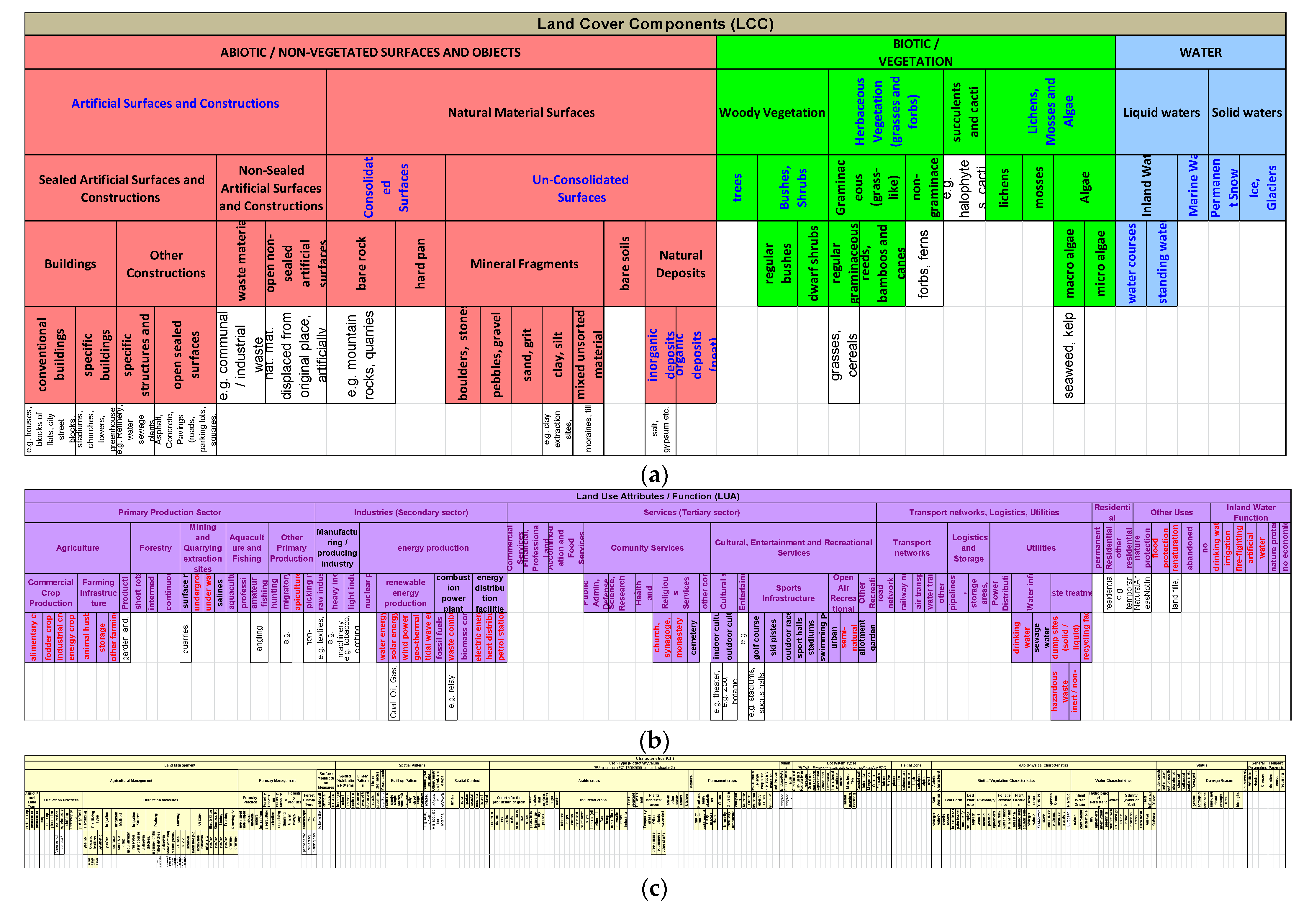
Figure 1 illustrates the three blocks of the EAGLE matrix. From top to bottom, the grain size is gradually refined to meet the requirements of the definition of different scales of land-cover types. These components, attributes and characteristics can be selected arbitrarily according to the definition of the type of land-cover products when designing the local ontologies. Moreover, to enable the task of land-cover map integration, the EAGLE matrix specific modules can be extended and customised in terms of adding attributes and axioms to enable the identification of design inconsistencies. The system architecture is depicted in Figure 2, which describes the main components and the relations between them.

2.1.3. Local Ontologies

Local ontology is used to describe the conceptual model of each data source. Firstly, we need to make a comprehensive analysis of the required data sources by considering the terms of each data source and the hierarchical relationship between each class. The hierarchical structure of concepts in the corresponding local ontology establishes a reference to the data source classification system. Secondly, each local ontology land-cover concept is decomposed into the global vocabulary–EAGLE matrix to express the attributes and relationships clearly. To comply with the shared vocabulary, each category’s semantic needs to be analysed.
For example, the land-cover products involved in this study as a case study include GlobeLand30, NLCD and FROM-GLC-Seg. The classes in the land-cover product usually employ a hierarchical structure. Therefore, the ontologies of each source land-cover data consist of concepts that are also arranged in a hierarchical structure mimicking the arrangement of the classification system. Thus, when the land-cover categories are encoded in ontologies, the categories become concepts.
Figure 3 illustrates a specific example of a coniferous forest in the local ontology of FROM-GLC-Seg. Each concept in the local ontology is specifically referenced for the corresponding definition of its legend.
In Figure 3, the rectangle represents the concept, the ellipse represents the attribute, the thick black arrow represents the inheritance relationship, the thin black arrow represents the attribute relationship and the words on the line represent the name of the relationship. In FROM-GLC-Seg, coniferous forest is defined as areas where trees are more than 3 m high and forest coverage is more than 15.0%, and the corresponding attributes include leaf type, tree height, mosaic or not and so on. Other EAGLE matrix elements have nothing to do with the semantics of the definition of a coniferous forest are not shown here. Coniferous forest is a subclass of forest in FROM-GLC-Seg, which has the components ‘tree’ related to biology/vegetation-woody plant—tree in the global vocabulary–EAGLE LCCs block.
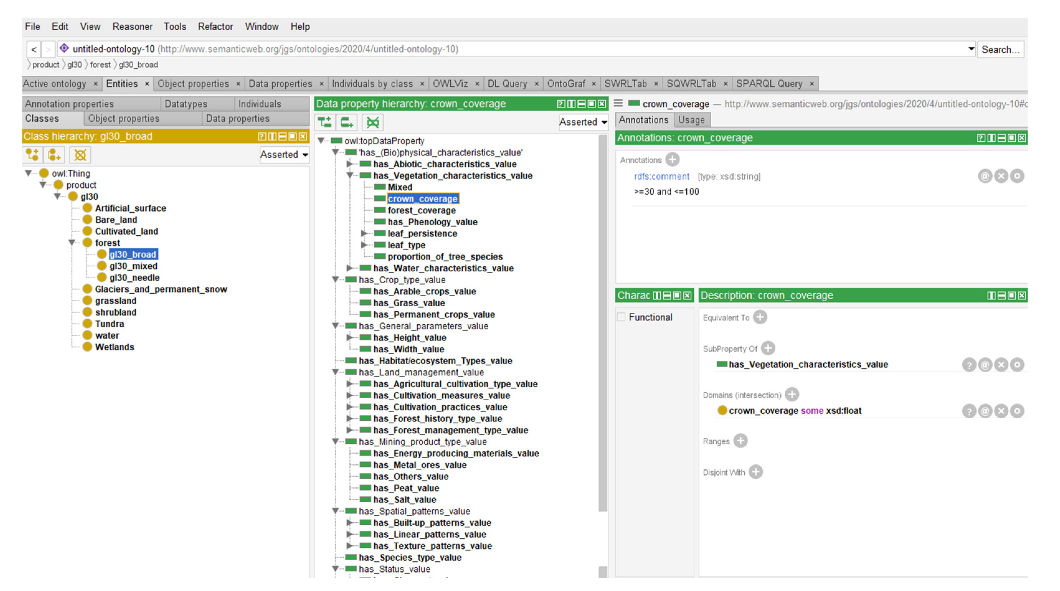
GlobeLand30 has 10 first-level land cover types. The specific definition of each category is referenced from the web site (http://www.globeland30.org) (accessed on 28 May 2021). As this study will take the second-level refinement of forest type as an example, the forest first-level is divided into coniferous forest, broad-leaf forest and mixed forest. The GlobeLand30 land-cover ontology is shown in Figure 4. The first column is the Globeland30 land-cover concepts and the hierarchical relationship between them. The second column present the data attributes of the concepts. The third column lists some restrictions of the attribute. For example, for the crown coverage, its annotation is ≥30 and ≤100. The definition field and value field of specific attributes can be set on the corresponding attributes. Which global vocabulary elements are needed to define the semantics of each land-cover type must be analysed by experts according to their definition, and the semantics of each land-cover category need to be decomposed.
The NLCD classification system merged existing schemes, including the NOAA Coastal Change Analysis Program (C-CAP) classification protocol and the Anderson system. NLCD 2011 has 8 first classes and 16 s classes [46]. NLCD land-cover ontology is shown in Figure 5.
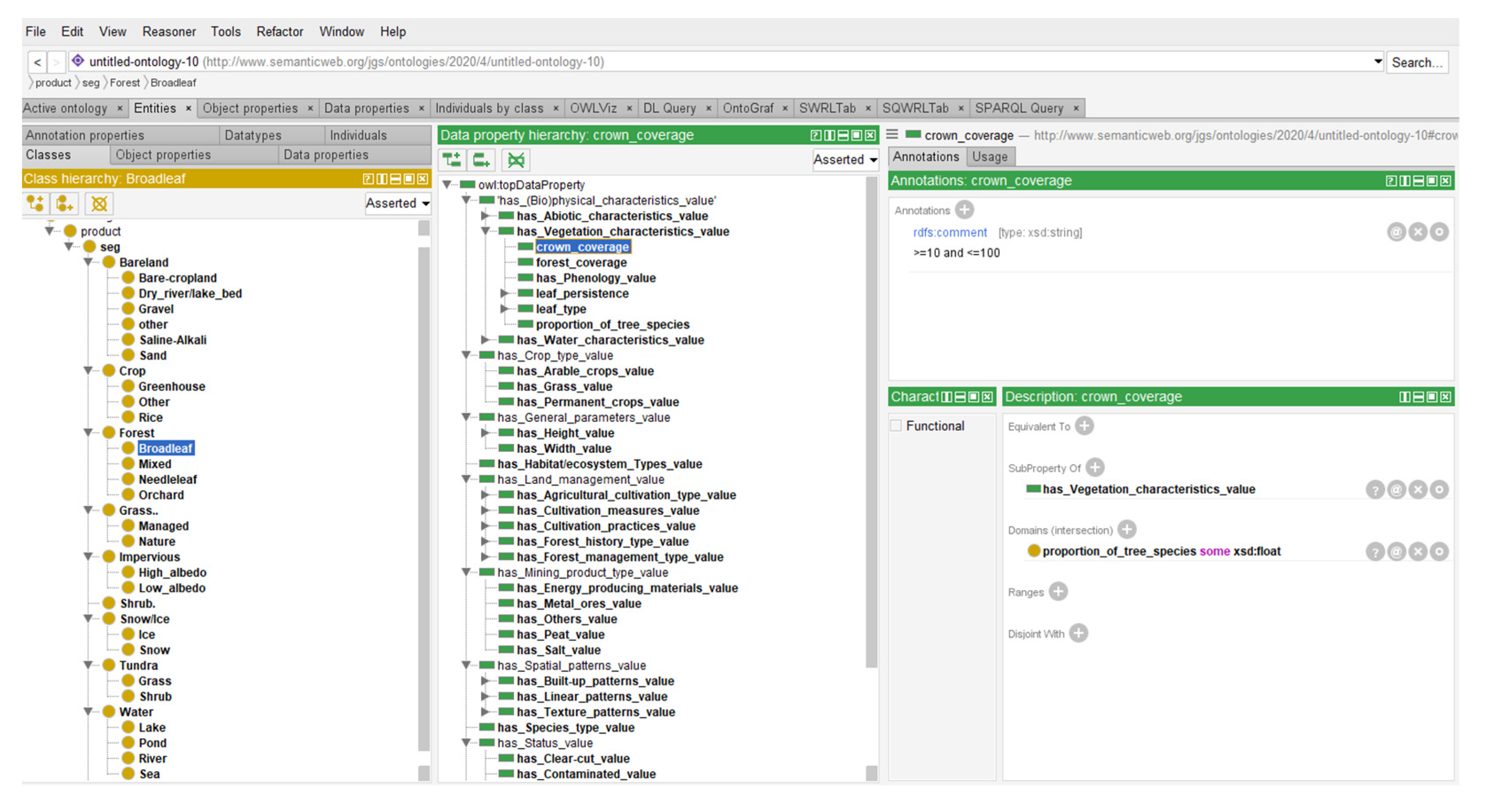
Based mainly on the end-component analysis and the potential of only six bands of spectral data from TM and ETM+ imagery, the classification scheme of FROM-GLC-Seg has a two-level hierarchy involving 10 first-level classes and 27 s-level classes [47]. The land-cover ontology of FROM-GLC-Seg is shown in Figure 6.

2.1.4. Ontology Mapping-Similarity Calculation

Through ontology mapping of land cover, we can get all kinds of relationships among the land-cover concepts between ontologies. In this study, the ultimate goal is to fuse different land-cover products to generate a new land-cover product. The ontologies are used to evaluate the semantic similarity between land-cover categories (concepts) from different products (local ontology). The method of hybrid similarity calculation is adopted. Firstly, using the hybrid ontology model established above, the attribute similarity between different ontology concepts can be calculated by using the elements in the shared global vocabulary EAGLE matrix. In addition, the mapping of ontology terms can be obtained by comparing terms with external resources, such as dictionaries. Instance-based mapping is also used to calculate the similarity between concepts. Weighted synthesis of the three similarities is used to get the comprehensive semantic mapping results.

Ontology Mapping Based on Term

In this paper, the similarity of term is divided into definition similarity and lexical similarity. In the calculation of definition similarity, the widely used Wu-Palmer [48] algorithm based on definition distance is used, which is based on WordNet [41]. WordNet is a large lexical database of English, which not only includes the definition of words but also labels the semantic relations among words. On the contrary, the groupings of words in a thesaurus follow meaning similarity.
Firstly, the term definition in WordNet of each pair of concepts between two ontologies are segmented, that is, stemmed to get the two word sets { A i = | i = 1 , 2... , n } and { B j = | j = 1 , 2... , n } . The corpus of the current study only contained nouns and adverbs, and so according to the rule that the parts of speech of words can be derived from each other [49], the adjective can be replaced with a noun with a similar meaning by searching its synonyms in WordNet.
The similarity of two words from word Sets A and B is calculated according to the Wu-Palmer algorithm [48] as Formula (1).
Sim ( A i , B j ) = 2 × depth ( ( A i , B j ) ) depth ( A i ) + depth ( B j )
where depth ( A i , B j ) is the nearest common ancestor of words Ai and Bj, with depth ( A i ) and depth ( B j ) representing the depths of words Ai and Bj in the WordNet semantic tree, respectively. Find the largest similarity value between each word in the B set and A set, and then the average is the definition similarity of the term as in Formula (2):
S i m d e f i n i t i o n ( A , B ) = j = 1 n S i m ( A , B j ) / n
Lexical similarity is also considered and the calculation formula [50] is as follows
S i m l e x i c a l ( A , B ) = M a x ( 0 , ( 1 2 × t r a n s ( A , B ) | t o k e n ( A ) | + | t o k e n ( B ) | ) )
where | t o k e n ( A ) | and | t o k e n ( B ) | are the number of words in Terms A and B, respectively, and lexical similarity is the minimum number of editing operations (insert, delete and replace) required to convert Term A to Term B.
After the definition similarity and lexical similarity are calculated, the weighted average is combined to obtain the similarity of the ontology terms S i m t e r m ( A , B ) . In this way, the term similarity between each pair of concepts between two ontologies can be calculated to form a similarity matrix.

Similarity Calculation Method Based on Attributes

In local ontology, the semantic attribute of each land-cover concept is expressed by some EAGLE elements from LCCs, LUAs and CH blocks in the global vocabularies. The theoretical basis for calculating concept similarity based on attributes is as follows: if two concepts have similar attributes, then the two concepts are similar; if the value of attributes is similar, then the attributes are also similar. The calculation effect depends on the completeness, adequacy and accuracy of decomposing the ontology attributes.
Attributes includes attribute name, attribute type and attribute value. There are different types of land-cover attributes, including character type, numerical type, interval type, and Boolean type. It is only meaningful to calculate attribute similarity between the same attribute types.
(1) Numerical attribute types are commonly used in land-cover ontology. Similarity calculation can be completed by a mathematical comparison. If the attribute values are the same [51], then the similarity value is 1. The formula is:
sim ( p i m , p j n ) = { 1 , p i m = p j n 1 | p i m p j n | M a x ( p i m , p j n ) , p i m p j n
where p i m , p j n represent the same global vocabulary but of two ontologies. M a x ( p i m , p j n ) is the maximum value of p i m , p j n .
(2) Interval-type attribute values are common, such as canopy coverage, which is generally a range. If there is no intersection between an interval-type attribute of two different land-cover concepts, then the similarity is 0; if the interval range is exactly the same, then the similarity is 1. Similarity can be calculated by Formula (5).
sim ( p i m , p j n ) = p i m p j n | max ( p i m , p j n ) min ( p j n , p j n ) |
where max ( p i m , p j n ) refers to the maximum value of the range, and min ( p j n , p j n ) refers to the minimum value of the range. represents the overlapping value of the interval length.
(3) Boolean attribute values are rare in land-cover concepts, and the similarity calculation method can refer to Formula (6). For the similarity calculation of Boolean type, they belong to the ‘Yes or No’ relationship, and the semantic similarity is calculated as follows:
sim ( p i m , p j n ) = { 0 , p i m p j n 1 , p i m = p j n
Then, the attribute similarity between concepts is obtained by Formula (7), which is a weighted sum of all the attributes and components of the share global vocabulary.
S i m a t t r i b u t e ( A , B ) = k = 1 n w k S i m ( p i m , p j n )  
where p i m , p j n are the components and attribute of concepts A and B from two different local ontologies i and j, respectively; and w k [ 0 , 1 ] is the weight of the kth attribute or components. The sum of wk is 1.

Instance-Based Ontology Mapping

Instance-based ontology mapping method finds the semantic association between heterogeneous ontologies by comparing the extension of concepts, that is, ontology instances. The 1:1 mapping relationship between ontologies is found with reference to the idea of GLUE [50]. The similarity calculation is based on the joint probability distribution between concepts, and the measure of probability distribution is used to judge the similarity between concepts. The joint probability distribution between Concepts A and B includes P ( A , B ) ,   P ( A ¯ , B ) ,   P ( A , B ¯ ) ,   and   P ( A ¯ , B ¯ ) . Take P ( A ¯ , B ) for example; it represents the random selection of an instance from all instances, where the probability of belongs to B but not to A. In this study, the method of calculating the instance similarity is to use the land-cover sample points, count the above four joint probabilities between Concepts A and B and then calculate the similarity according to the following formula:
S I M i n s t a n c e ( A , B ) = P ( A B ) P ( A B ) = P ( A , B ) P ( A , B ) + P ( A , B ¯ ) + P ( A ¯ , B )
S I M i n s t a n c e ( A , B ) represents the instance-based mapping similarity. For example, to obtain the mapping relationship between the two heterogeneous ontology concepts of deciduous forest (represented by A) in NLCD and broad-leaf forest (represented by B) in GlobeLand30, a certain number of sample points should be selected for instance-based similarity calculation. The proportion of the sample points of deciduous forest in NLCD but not of broad-leaf forest in GlobeLand30 to the total sample points is counted, that is, P ( A , B ¯ ) . The proportion of sample points that are not deciduous forest in NLCD but broad-leaf forest in GlobeLand30 to the total sample points is counted, that is, P ( A ¯ , B ) , and the instance similarity of Concepts A and B can be calculated according to Formula (7). When A and B are completely unrelated, the similarity is 0. When A and B are equivalent concepts, the similarity is 1. Instance-based similarity is more likely to be the result of real data feedback. Compared with the result of term and attribute similarity, it directly examines the similarity of land-cover data itself. However, because it is manually verified, the selection of verification points and the error of manual recognition will also affect the subsequent integration results.

Synthesis of Mapping Methods

For each pair of concepts that need to be mapped, the results of each similarity calculation, including term, attribute and instance, are accumulated. To emphasise reliable similarity and reduce the influence of unreliable similarity, the weighted sum method is used. The comprehensive semantic similarity S i m ( A , B ) is as follows:
S i m ( A , B ) = ω t e r m S i m t e r m ( A , B ) + ω a t t r i b u t e S i m a t t r i b u t e ( A , B ) + ω i n s t a n c e S i m i n s t a n c e        
where ω t e r m + ω a t t r i b u t e + ω i n s t a n c e = 1 . The setting of weights needs to be determined by domain experts according to the reliability of each similarity.
The comprehensive semantic similarity as well as the term, attribute and instance similarity calculation result is a matrix, and each value in the matrix is the similarity value of each pair of concepts.
Table 1 shows the similarity matrix. Take NLCD and FROM-GLC-Seg as the source data and GlobeLand30 as the fusion target data as an example; only forest-related types are listed.

2.2. Integration on the Data Level

2.2.1. Using Geostatistics to Obtain the Local Accuracy Map of Source Data

The accuracy of land-cover products is usually expressed by the overall accuracy of statistical sampling, but the overall accuracy cannot reflect the spatial variability of map accuracy, and the distribution of classification error on the map is not uniform. With the availability of reused reference sample data [22], geo-wiki, Flickr photo sharing and other volunteer-based reference data, the number of reference sample sites has increased significantly, and the spatial variability of large-scale land-cover map accuracy can be simulated by using combined reference datasets.
To evaluate local accuracy, the spatial correspondence between the source data and the reference dataset is coded with the indicator. If the class of the reference sample point matches the class of the source data, indicator code 1 is assigned to the sample point. Otherwise, the sample point indicator code will be 0. Next, the spatial autocorrelation of the indexes is analysed by using the semivariogram. Indicator Kriging method is used to create a local accuracy map for each source data. The local accuracy result is described between 0 and 1, which represents the correct local probability of a specific image. The detailed process can be found in references [22].

2.2.2. Land-Cover Data Integration

In this study, land-cover data are not transformed from its initial format into to actionable intelligence information, such as the standard triple model of RDFs. Ontology-based integration is only carried out on the semantic level as presented above.
The final integration model of land-cover products considers the similarity of the schema layer between different local ontologies and the local accuracy of each source product and combines the two to get the result. Two kinds of integration models are considered in this study as listed below.

Integration Model I

Integration Model I considers two factors: semantic similarity and local accuracy. The model is as Formula (10).
g y = ( A k ( x ) , B ( x ) ) × U ( C k ( x ) )
where x represents a pixel in the land-cover map. g y ( x ) represents the possibility that x belongs to class y. y ( n 1 , n 2 , n 3 , n k ) and ni are the categories in target land-cover product. S i m k ( A k ( x ) , B ( y ) ) represents the comprehensive similarity of pixel x’s category in a land-cover product k with the class y in the target product, which is calculated by Formula 8. U ( C k ( x ) ) is the local accuracy of pixel x on the land-cover product k. k is the number of source land-cover products.
To describe the probability that pixel x belongs to which category in the target legend, Formula (11) indicates that when the maximum value is taken, the y class is the final class.
G ( x ) = ax y Ω g y ( x )
Integration Model I considers the influence of each source data, adds the influence of each of source data and finally compares the probability result of each type in the target legend, which is a way of fuzzy set.

Integration Model II

In integration model I shown in Formula (10), the results of several source data are summed up. In this way, the effect of semantic similarity or local accuracy of a source product may be diluted. To highlight the semantic similarity between each source product and the target product as well as the local accuracy of the source product, integration Model II does not use the form of summation but takes the maximum value. The integration model is expressed in Formulas (12) and (13).
Take Table 1 as an example. Here the comprehensive semantic similarity matrix mentioned in Section 2.1.4 is expressed as Matrix M. For a pixel x in the target land-cover map (i.e., GlobeLand30 product), if its category in NLCD2011 is deciduous forest and in FROM-GLC-Seg is broad-leaf forest, then the maximum values among S 11 N ,   S 12 N   and   S 13 N   and the maximum values of S 11 F , S 12 F   and S 13 F   will be extracted, respectively, as in Formula (12).
S i m k M a x ( x ) = M a x ( S i m k ( A k ( x ) , B ( y ) ) )
where y ( n 1 , n 2 , n 3 ) and n1 is broad-leaf forest, n2 is coniferous forest and n3 is mixed forest. k = 1 , 2 here represents NLCD2011 and FROM-GLC-Seg, the two-source land-cover products. S i m k ( A k ( x ) , B ( y ) ) is the comprehensive semantic similarity between the class of pixel x in a source land-cover product and the class (y) in the target land-cover product. S i m k M a x ( x ) is the result of taking the maximum. This step can get the maximum similarity of each source data with target data.
Then, S i m k M a x ( x ) is multiplied with the product k local accuracy of pixel x using Formula (13), and the final result of fusion can be obtained.
G ( x ) = M a x ( S i m k M a x ( x ) · U ( C k ( x ) ) )
where U ( C k ( x ) ) represents the local accuracy of pixel x of k product k. In Formula (13), the maximum value of the two values is selected as the final forest type.
In the integration Model II, firstly, the results of the comprehensive semantic similarity itself are compared and then the comparison results are multiplied by the local accuracy so that the effect of comprehensive semantic similarity and local accuracy on the integration result can be maximised. We will compare the effectiveness of the two models through experiments in the next section.

3. Results

3.1. Data

3.1.1. Source Land-Cover Data

In this study, the land cover data used in Zhu et.al [25] is adopted as an example. Three 30 m resolution land cover products, namely NLCD 2011, FROM-GLC-Seg and GlobeLand30, are selected as a case study. Integration NLCD and FROM-GLC-Seg forest second-level categories to subdivide GlobeLand30 (2010) forest first class into coniferous, broad-leaf and mixed forests, is for testing the integration method. The conterminous United States region is adopted as the research area. The data source is the products close to year 2010 to reduce the product differences caused by time differences.
GlobeLand30 is a global land-cover product with 10 main categories, including cultivated land, forest, grassland, shrubland, wetland, water body, tundra, artificial surface, barren land and permanent snow and ice. The average accuracy of 80.0% for full classes or one single class is achieved by third-party researchers from more than 10 countries through a sample-based validation or a comparison with existing data [10]. The second-level classification of products is still under development.
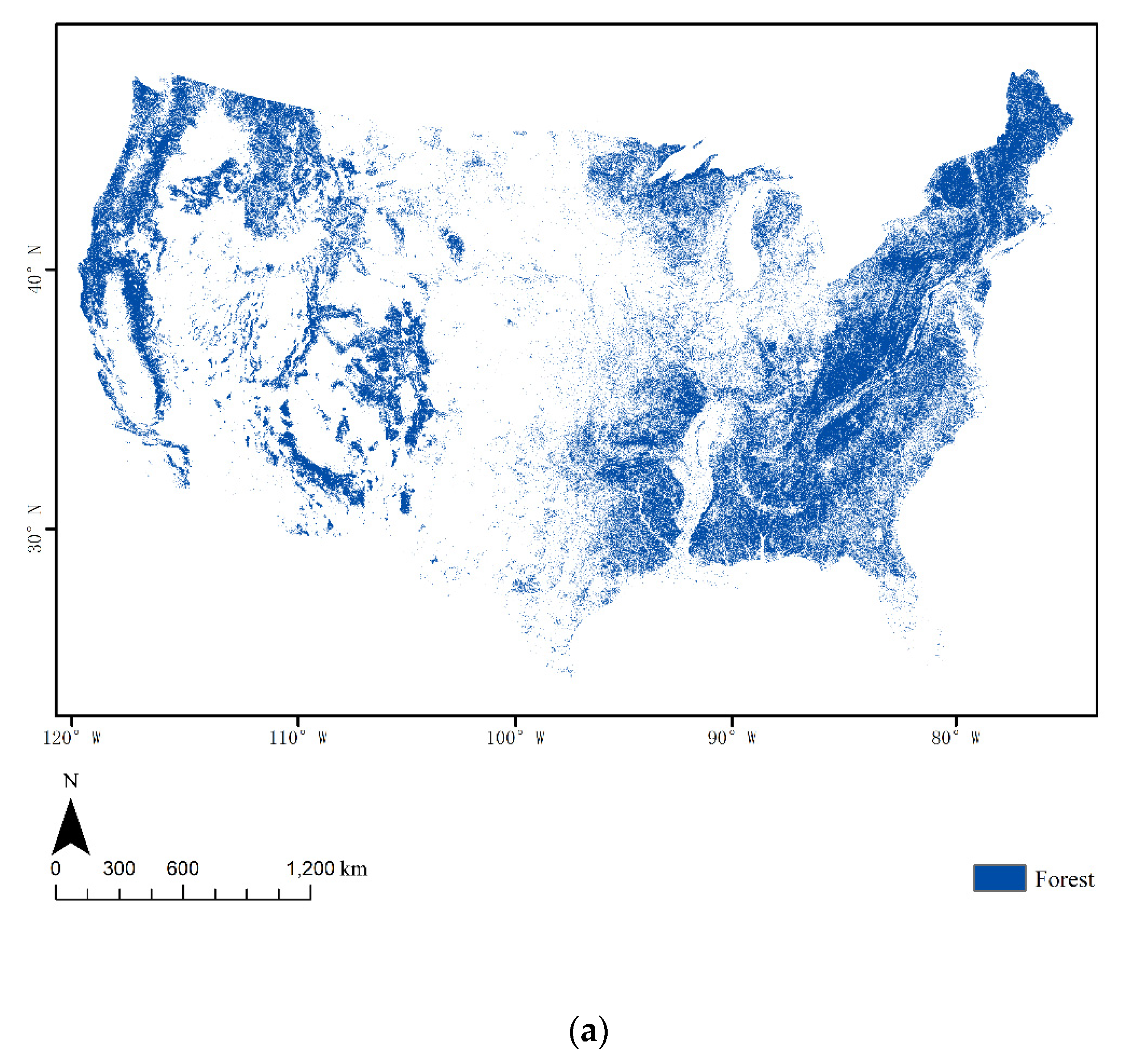
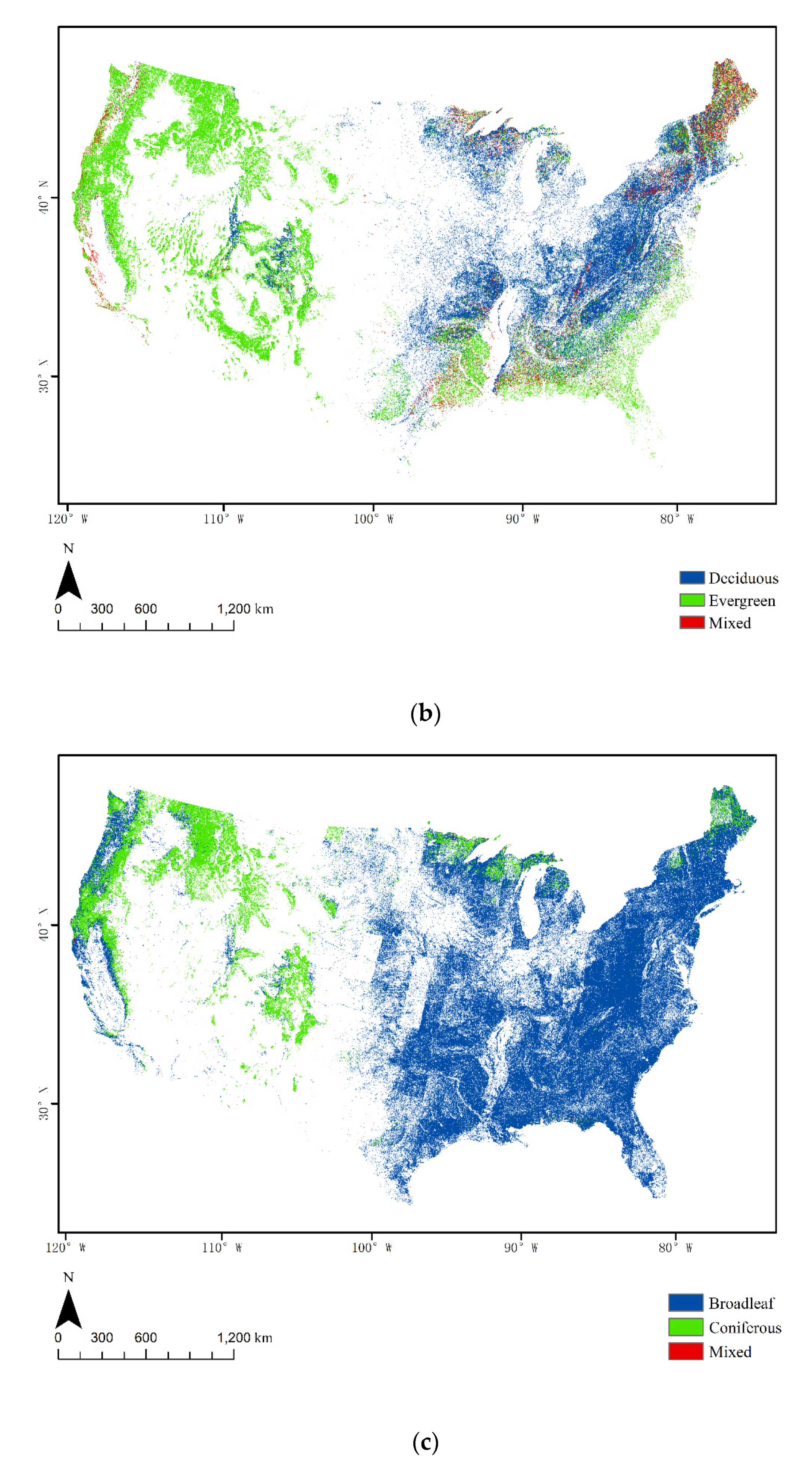
In GlobeLand30, the areas with more than 30% forest coverage are defined as forest types. The forest map of the study area is shown in Figure 7. According to the nomenclature of GlobeLand30, the second level includes broad-leaf forest, coniferous forest and mixed forest. The specific definitions are shown in Table 2.
The NLCD is a 30 m resolution U.S. nationwide land-cover product, which includes Alaska, Hawaii and Puerto Rico; it is developed dominantly by the United States Geological Survey. Five phase products have been released, such as NLCD1992, NLCD 2001, NLCD 2006, NLCD 2011 and NLCD.2016 [52]. The classification system of NLCD 2011 has eight first classes and 16 s classes (excluding the four other classes of Alaska) [46]. The forest class is divided into evergreen, deciduous and mixed forests according to the leaf phenology, as defined in Table 2. The distribution in the study area is plotted in Figure 7b. The values of user accuracy of deciduous, evergreen and mixed forests are 76.0%, 76.0% and 29.0%, respectively, according to the thematic accuracy assessment provided by Wickham et al. [53].
The 30 m resolution land-cover products of FROM-GLC are obtained by classified remote sensing image through automatic supervised classification. FROM-GLC adopts the automatic supervised classification method with relatively low accuracy. Subsequently, the algorithm is improved, and the upgraded product FROM-GLC-Seg is produced with the overall accuracy raised to 67.1% [47]. The legend system of FROM-GLC-Seg is similar to that of GlobeLand30, with 10 first classes and 27 s classes. The second class of forests is divided into broad-leaf, coniferous and mixed forests according to leaf type. The map is demonstrated in Figure 7c, and the specific definition is presented in Table 2.
NLCD and FROM-GLC-Seg have second-level classes of forest type. However, the names and semantics of the second-level forest classification are different. NLCD subdivides the forest into deciduous, evergreen and mixed forest according to the leaf phenology. FROM-GLC-Seg subdivides forest into broad-leaf, coniferous (needle leaf) and mixed forest according to leaf type.
According to 2002 statistics, the existing forest area of the conterminous United States is 303,123 million Hm2, accounting for 33% of the total land area, and the forest volume ranks the fourth in the world [54]. Forests in the United States are mainly distributed in three areas. Coniferous forests are dominant from the Western Rocky Mountains to the Pacific coast while pine trees are dominant in the South Atlantic and Gulf Coast. The eastern part of the Mississippi River is dominated by broad-leaved trees [55].

3.1.2. Reference Data

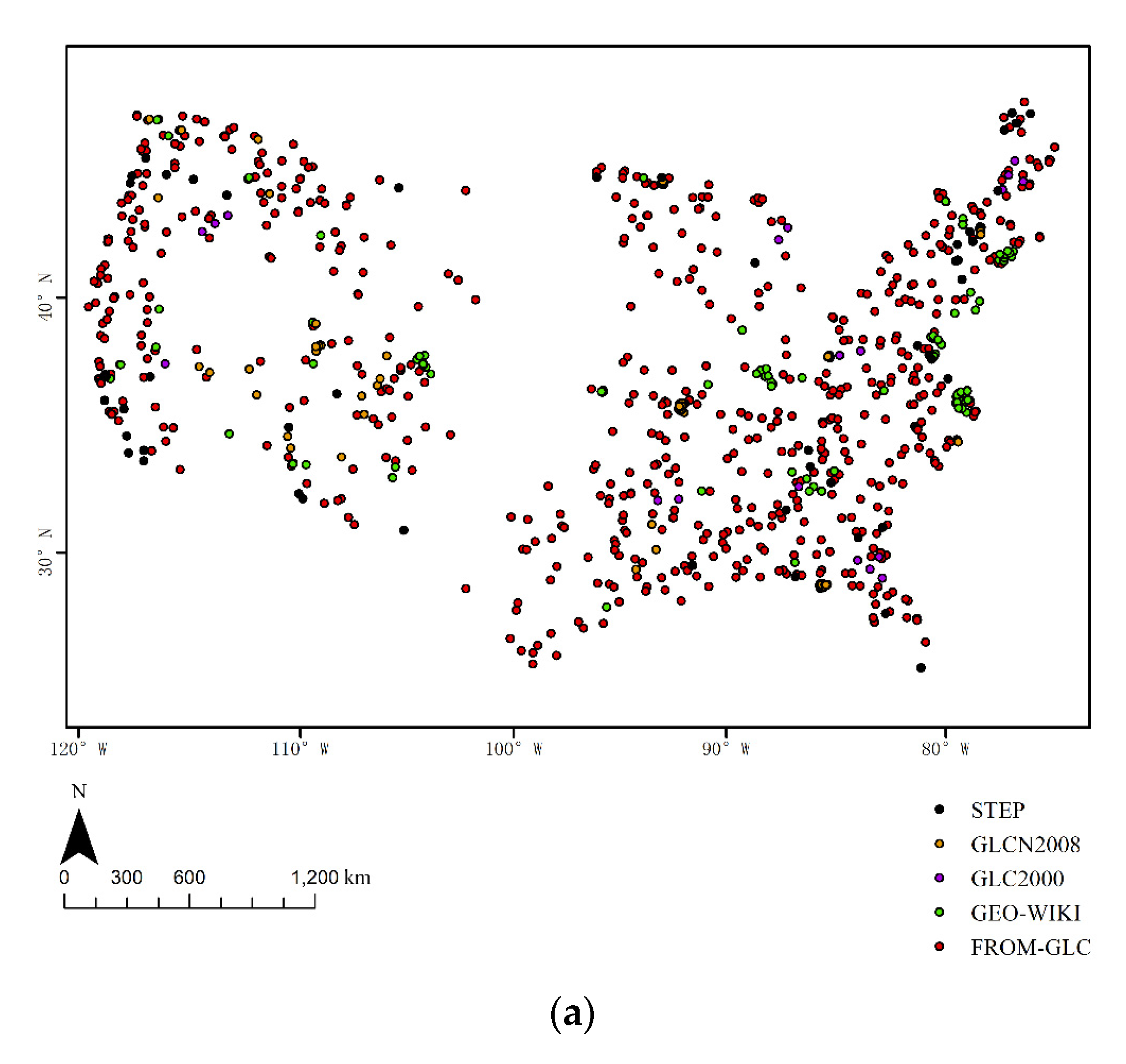
A large number of evenly distributed ground verification points are needed to evaluate the local accuracy of source products. The accuracy of the integration results is also evaluated through the ground verification points. The verification points of land cover provided by Zhu et al. [25] are used. The total number is 2984, as shown in Figure 8. The verification points are obtained from two kinds of methods. The first method involves reusing existing reference sample datasets built for calibrating and validating GLC maps. The verification points in this paper are collected from the GLC 2000 reference dataset, the STEP reference dataset, the GLCNMO 2008 dataset, the Geo-Wiki crowdsourced data and the global validation sample set developed by Tsinghua University [25], as exhibited in Figure 8a,b. The total number is 1060, where the numbers of broadleaf, coniferous and mixed forests are 447, 373 and 240, respectively. The second method is visual interpretation, which is another way to acquire reference sample pixels to increase the number of reference sample data. Several coniferous and broadleaf forest random sample points (mixed forest is not included due to the difficulty in interpretation) generated by the ArcGIS 10.1 toolbox (create random points) are visually interpreted on high-resolution Google Earth images and added. A total of 1024 coniferous forests and 900 broadleaf points are added to the reference sample pixel set as presented in Figure 8c.
To evaluate the local accuracy of NLCD products, the attribute of defoliation of each reference sample pixel is additionally judged by an expert interpreter. Among them are 828 deciduous, 1825 evergreen and 331 mixed forests.
Owing to the limited number of verification points used to evaluate the local accuracy of source products, it cannot meet the density requirements of 30 m resolution. To evaluate the local accuracy reasonably, this study resamples the resolution of all land-cover products and obtains the data of 300 m resolution.

3.2. Result of Schema-Level Integration

3.2.1. Ontology Mapping Based on Term

The concept from different ontologies involved in this paper includes six subcategories of forest types: broad-leaf forest, coniferous forest, broad-leaf and coniferous mixed forest, deciduous forest, evergreen forest and deciduous evergreen mixed forest. The concepts are translated by using the semantic dictionary WordNet to obtain the specific definition of each concept in the field, and the specific word set is obtained by word segmentation, stemming. Table 3 presents the word set obtained after extracting the stem.
Table 4 shows the results of the definition similarity and lexical similarity calculation between the two kinds of source data, namely NLCD2011 and FROM-GLC-Seg, and the integrated target data Globeland30, and then averages the result to get the term similarity. The result column of average value is marked with light green colour, and the maximum average value of each row is marked with deeper green colour. In the ‘definition’ similarity column, the similarity between the mixed forest of GlobeLand30 and the forest type of each product are greater or similar than other forest types. The reason may be that the types used in this study all belong to the subclass of forest types, and each type is semantically close and confused with one another. Therefore, it is difficult to make a detailed distinction. Taking NLCD as an example, because the word set of mixed forest includes all the word set of deciduous forest and evergreen forest, it is always similar to or larger than the results of deciduous forest or coniferous forest.

3.2.2. Ontology Mapping Based on Attributes

In the shared global vocabulary, the forest types in this study mainly include the following attributes: crown coverage, proportion of tree species, tree height, forest coverage, leaf type, leaf persistence and whether mosaic or not etc. The EAGLE matrix of these related LCC, LUA and CH are shown in Table 5. They are listed from top to bottom according to the hierarchy structure of EAGLE matrix. The first row is LCC, LUA and CH modules; the second row is the second level division, and so on.
Attribute types are divided into three types: numerical type, interval type and Boolean type. Among them, the numerical types are leaf type, leaf persistence and the proportion of tree species. The interval types are crown coverage, forest coverage and tree height. Boolean type is whether mosaic or not and ‘tree’ component. The attribute similarity is calculated according to Formulas (4) to (7). Weights are set to be equal. The result is shown in Table 6. In Table 6, the maximum value of each row is marked with deeper green colour.
As can be seen from the above table, there is no obvious difference in the results of attribute similarity because the example of forest we selected is more challenging. All the categories belong to a kind of forest. The data attributes of the second-level class of several forest types are very similar. According to common sense, most of the deciduous leaves belong to the broad-leaf type, and most of the evergreen forest belongs to coniferous type. For example, the overlap of deciduous forest in NLCD2011 and broad-leaf forest of GlobeLand30 is almost equal to that of deciduous forest in NLCD2011 and coniferous forest of GlobeLand30. However, due to the introduction of the other two kinds of similarity mapping, the combination of multiple kinds of similarities improves the calculation results of attribute similarity.

3.2.3. Ontology Mapping Based on Instance

Instance-based similarity is obtained through the statistics of the types of verification points in different source data. The results are shown in Table 7. FROM-GLC-Seg and GlobeLand30 have similar type semantics and names, so we get consistent results from instance-based mapping. Deciduous, evergreen and mixed forests in NLCD all have the greatest similarity with broad-leaf forest in GlobeLand30. These findings indicate that no direct connection exists between evergreen, deciduous, broad-leaf and coniferous forests. Evergreen forest includes evergreen broad-leaf forest and evergreen coniferous forest. The evergreen broad-leaf forest is mainly distributed in subtropical humid areas, which make the part of evergreen forest in NLCD considered as broad-leaf forest in GlobeLand30. Deciduous broad-leaf forest is generally distributed in temperate monsoon climate regions with cold winter. According to the climate distribution of the United States, deciduous broad-leaf forest is distributed in the northeast of the United States while evergreen broad-leaf forest is distributed in the southeast and southwest of the United States. This distribution leads to the phenomenon that deciduous forest may belong to broad-leaf or coniferous forest, and evergreen forest may also belong to broad-leaf or coniferous forest, which has a certain impact on the final results.

3.2.4. Synthesis of Mapping Results

The term-based, attribute-based and instance-based mapping methods obtained above are substituted into Formula (8) for weighted calculation to obtain the final comprehensive mapping. Weights are set equally. The results are shown in Table 8.
The mixed forest category is defined as a mixture of broad-leaf and coniferous or deciduous and evergreen forest. These kinds of dual definitions make it difficult to fully capture the semantics of the category. From the final results, it can be seen that through the comprehensive calculation of term, attribute and instance similarity, the interference of other forest types to mixed forest is reduced to a certain extent.

3.3. Result of Data Level Integration

3.3.1. Local Accuracy

Three-fourth of the abovementioned 2984 reference sample pixels (i.e., 2238 pixels) are evenly selected for local accuracy calculation and the remaining one-fourth set is used for accuracy evaluation. ArcMap 10.1 Geostatistical and Spatial Analyst tools are used to generate the local accuracy map of each source dataset.
The local accuracy or spatial correspondence maps of NLCD 2011 and FROM-GLC-Seg products are demonstrated in Figure 9a and b, respectively. The greener the colour, the higher the probability of the point; whereas, the redder the colour, the lower the probability of the pixel. The possible low correspondence areas should be the main focus of map improvement regions.

3.3.2. Integration Results

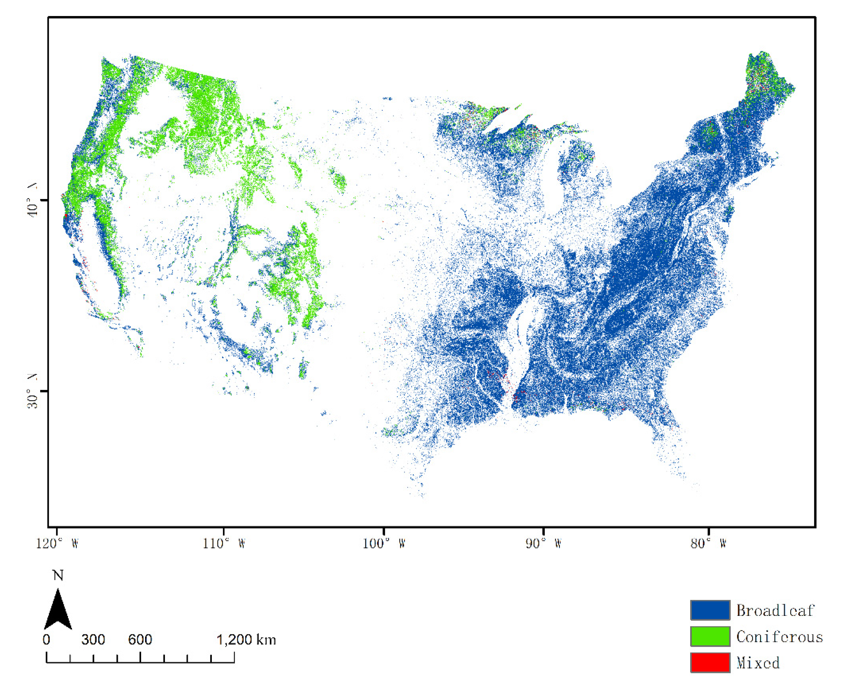
According to the above calculation results, the pixels corresponding to the GlobeLand30 forest pixels are extracted from NLCD2011 and FROM-GLC-Seg and then substituted into integration Model I and Model II to calculate the probability that each pixel belongs to each category. Comparing the probability can determine the final category of each pixel. Finally, the second-level class refinement results of forest types in GlobeLand30 (2010) are shown in Figure 10 and Figure 11.
Figure 10 and Figure 11 show that broad-leaf forests are mainly distributed in most areas of the eastern part and some marginal areas of the western part. Coniferous forests are mainly distributed in the western and northeastern parts. The distribution of mixed forest is less and scattered. For example, the coastal areas of western California, parts of Minnesota and Michigan in the north central and coniferous forest areas of northeastern Maine are also mixed with some mixed forests. Some mixed forests are also distributed in Louisiana in the southeast, Texas in the south central and New Mexico in the southwest.
However, there are some differences between the results of the two integration models, mainly in the distribution area of mixed forest. Compared with the results of integration Model I, the mixed forest of integration Model II added some new areas. For example, in the western and northern regions of Florida, there are some new mixed forests compared with the results of Model I. Some mixed forests are also distributed in Arkansas and Oklahoma. Compared with the sporadic distribution of Model I, the distribution of Model II is more intensive, which is similar to the distribution area of mixed forests in our verification point.

3.4. Accuracy Analysis

Confusion matrix is used to evaluate the accuracy of integration results. The results are summarised in Table 9 and Table 10, which show the accuracy verification results of integration Models I and II, respectively.
As can be seen from Table 9, the values of user accuracy of broad-leaf, coniferous and mixed forests are 82.6%, 72.0% and 48.3%, respectively. The reason for the low accuracy of mixed forest is that the semantic concept of mixed forest is fuzzy, making it difficult to distinguish from broad-leaf and coniferous forest. On the other hand, because the total number of pixels of mixed forest is relatively small, it is difficult to collect sample points, which affects the accuracy of judgment.
As can be seen from Table 10, the values of user accuracy of broad-leaf, coniferous and mixed forests are 82.6%, 72.0% and 60.0%, respectively. Compared with the results of Model I, the accuracy of broad-leaf and coniferous forest has no change and only the mapping accuracy is improved, increasing by 1.2% and 1.4%, respectively. However, the accuracy of the mixed forest is increased by 11.7%, and the overall accuracy is increased by 1.0%. In addition, some differences can be seen by comparing the number of pixels of fusion results. The number of broad-leaf, coniferous, and mixed forests of integration Model I are 18,848,060, 4,657,822 and 125,362, respectively, and the number of broad-leaf, coniferous and mixed forests of integration Model II are 18,825,065, 4,654,899 and 151,280, respectively. The number of pixels of broad-leaf and coniferous forests changed little, but the number of pixels of mixed forest increased by 20.7%.
Compared with Zhu et.al [25] using the same datasets to do the same integration task, the user accuracy of broad-leaf, coniferous and mixed forests are 79.9%, 69.9%, and 59.3% of their results. They also considered the local accuracy of the source land cover product and EAGLE matrix was used to translate the semantics. However, the bar code method was used to calculate the similarity between different land cover categories. From the comparison of the accuracy of the results, it can be seen that the ontology based method can better express the semantic relationship between land cover types and is more suitable for automatic integration of big data in the future.

4. Discussions

This study chooses the integration of forest categories as an example, which is a very challenging one. Mixed forest is a special type, and its semantics is relatively vague. For example, when gathering sample data for land-cover accuracy assessment, a reference pixel could be labelled a ‘mixed forest’ even though it is very similar to a ‘coniferous forest’, so a dataset could be almost right even if it classified that object as a ‘coniferous forest’. Intuitively, a ‘mixed forest’ is much more similar to a ‘coniferous forest’ than to an ‘impervious surface’, so the two forest types would probably be harder to distinguish and result in some classification confusion. When the semantics of two categories overlap too much, it would lead to unacceptable error rates in the resulting maps. If the integration task is other types, then the situation of semantic analysis will be simpler than this study.
With the use of integration Model II, the accuracy of mixed forest is improved considerably without losing the accuracy of broad-leaf and coniferous forests. Although the number of mixed forests increased by 20.7%, the transformation from broad-leaf and coniferous forest to mixed forest was only about 1/10.000 of broad-leaf and coniferous forest and therefore had little impact on the final accuracy verification. The results should not change much when the number of pixels in broad-leaf and coniferous forests is almost the same. The accuracy of mixed forest is improved substantially because by taking the maximum value in integration Model II, stick out of semantic similarity and local accuracy, is more effective than Model I in judging the mixed forest type.
Take a real pixel as an example, the pixel is a mixed forest in NLCD2011, and the local accuracy is 0.793. It is broad-leaf forest in FROM-GLC-Seg, the local accuracy is 0.496. According to the semantic similarity in Table 7, the probability of the pixel belonging to broad-leaf forest is 0.506 × 0.793 + 0.844 × 0.496 = 0.820, coniferous forest is 0.413 × 0.793 + 0.514 × 0.496 = 0.582, and mixed forest is 0.552 × 0.793 + 0.540 × 0.496 = 0.706. Using integration Model I, the maximum value of 0.820, 0.582 and 0.706 is the final class of the pixel, that is, broad-leaf forest. However, using the integration model II, we first extract the result with the highest probability in Table 7. For the data NLCD2011, the maximum probability of the pixel belonging to mixed forest is 0.552, and for FROM-GLC-Seg, the maximum probability of the pixel belonging to broad-leaf forest is 0.844. In integration Model II, the probability of the pixel belonging to mixed forest in NLCD2011 is 0.552 × 0.793 = 0.438, and the probability of the pixel belonging to broad-leaf forest in FROM-GLC-Seg is 0.844 × 496 = 0.419. Therefore, result shows that the pixel belongs to mixed forest. It can be seen that the first integration model weakens the function of the comprehensive semantic similarity. However, in integration Model II, the similarity and local accuracy can be maximized.

5. Conclusions

This paper uses ontology to express land-cover concept semantics and fuse different source data through ontology-based integration. The integration model considers two aspects: the semantic similarity between source data ontologies and target ontology and the local accuracy of the source data. Semantic mapping between ontologies include term, attribute and instance mapping. The final semantic mapping is obtained by weighted average. The local accuracy is obtained by verification sample points and indicator Kriging method. Two kinds of integration models are used.
In this study, the GlobeLand30 forest is taken as an example and subdivided into coniferous, broad-leaf and mixed forest by integrating NLCD and FROM-GLC-Seg land-cover products. The values of user accuracy of broad-leaf, coniferous and mixed forests are 82.6%, 72.0% and 48.3%, respectively, by integration Model I and 82.6% for broad-leaf, 72.0% for coniferous and 60.0% for mixed forest by integration Model II.
The innovation of this study is that, for the first time, ontology-based integration method is used in the fusion of remote sensing land-cover products. A shared vocabulary is constructed by using EAGLE matrix elements, realising the mapping between local ontologies and obtaining the semantic mapping results.
The method in this paper is limited by the number and distribution of verification sample points because the instance-based similarity and local accuracy calculations depend on the verification points. For example, the original data with 30 m resolution in this study are resampled to 300 m due to the lack of sample points to meet the required sample point density for local accuracy estimation. This condition is attributed to the total number of pixels in the experimental area of 30 m resolution, which are approximately more than 2 billion forest pixels. Around two million reference samples are needed to achieve about 0.1% of the number of sample points, which cannot be realised by collecting the existing verification data. The workload of visual interpretation is also large. Therefore, realising the integration of high-resolution land cover products using the proposed method in this paper is difficult. Thus, improving the estimation method of local accuracy is necessary.
There are also some shortcomings in this study; specifically, the definition of mixed forest is relatively vague and easy to confuse with other types. The ontology of land-cover data is mainly the semantic model of land-cover nomenclature; OWL and protégé respectively provide the language and tools to build the model. However, in order to use this model in the land-cover intelligent discovery system, other software tools, such as Jena Open Source Toolkit, are needed to convert OWL documents into models, store them in the database and use SPARQL or other query languages to realise semantic reasoning.

Author Contributions

Conceptualization, funding acquisition and methodology, L.Z.; data curation, methodology and writing—original draft, L.Z.; methodology and software, G.J. and D.G. All authors have read and agreed to the published version of the manuscript.

Funding

This research was funded by The National Key Research and Development Program of China under Grant (NO. 2016YFB0501404) and Beijing Key Laboratory of Urban Spatial Information Engineering, NO. 20210217.

Institutional Review Board Statement

Not applicable.

Informed Consent Statement

Not applicable.

Data Availability Statement

Not applicable.

Conflicts of Interest

The authors declare no conflict of interest.

References

  1. Zhu, Y.Q.; Pan, P. Concept Method and Application of Geospatial Data Ontology; Science Press: Beijing, China, 2019. [Google Scholar]
  2. Zhu, L.; Jia, T.; Shi, R.M. Global Surface Covering Product Update and Integration; Science Press: Beijing, China, 2020. [Google Scholar]
  3. Loveland, T.R.; Reed, B.C.; Brown, J.F.; Ohlen, D.O.; Zhu, Z.; Yang, L. Development of a global land cover characteristics database and igbp discover from 1 km avhrr data. Int. J. Remote Sens. 2000, 21, 1303–1330. [Google Scholar] [CrossRef]
  4. Hansen, M.C.; Defries, R.S.; Townshend, J.; Sohlberg, R.A. Global land cover classification at 1 km spatial resolution using a classification tree approach. Int. J. Remote Sens. 2000, 21, 1331–1364. [Google Scholar] [CrossRef]
  5. Friedl, M.A.; Sulla-Menashe, D.; Tan, B.; Schneider, A.; Ramankutty, N.; Sibley, A.; Huang, X. Modis collection 5 global land cover: Algorithm refinements and characterization of new datasets. Remote Sens. Environ. 2010, 114, 168–182. [Google Scholar] [CrossRef]
  6. Bartholome, E.; Belward, A.S. Glc2000: A new approach to global land cover mapping from earth observation data. Int. J. Remote Sens. 2005, 26, 1959–1977. [Google Scholar] [CrossRef]
  7. Bicheron, P.; Defourny, P.; Brockmann, C.; Schouten, L.; Vancutsem, C.; Huc, M.; Bontemps, S.; Leroy, M.; Frédéric, A.; Herold, M.; et al. Globcover—Products description and validation report. Foro Mund. Salud 2011, 17, 285–287. [Google Scholar]
  8. CCI-LC. Product User Guide; CCI-LC: Louvain-la-Neuve, Belgium, 2014. [Google Scholar]
  9. Ryutaro, T.; Thanh, H.N.; Toshiyuki, K.; Bayan, A.; Gegen, T.; Xuan, P.D. Production of global land cover data-glcnmo2008. J. Geogr. Geol. 2014, 6. [Google Scholar] [CrossRef] [Green Version]
  10. Chen, J.; Liao, A.; Chen, J.; Peng, S.; Chen, L.; Zhang, H. 30m Global Land Cover Remote Sensing Data Product-Globe Land30. Geogr. Inf. World 2017, 24, 1–8. (In Chinese) [Google Scholar] [CrossRef]
  11. Yu, L.; Wang, J.; Gong, P. Improving 30m global land-cover map FROM-GLC with time series MODIS and auxiliary data sets: A segmentation-based approach. Int. J. Remote Sens. 2013, 34, 5851–5867. [Google Scholar] [CrossRef]
  12. Gong, P.; Liu, H.; Zhang, M.; Song, L. Stable classification with limited sample: Transferring a 30-m resolution sample set collected in 2015 to mapping 10-m resolution global land cover in 2017. Sci. Bull. 2019, 64, 370–373. [Google Scholar] [CrossRef] [Green Version]
  13. Gorelick, N.; Hancher, M.; Dixon, M.; Ilyushchenko, S.; Moore, R. Google earth engine: Planetary-scale geospatial analysis for everyone. Remote Sens. Environ. 2017, 202. [Google Scholar] [CrossRef]
  14. Xu, P.; Herold, M.; Tsendbazar, N.E.; Clevers, J. Towards a comprehensive and consistent global aquatic land cover characterization framework addressing multiple user needs. Remote Sens. Environ. 2020, 250, 112034. [Google Scholar] [CrossRef]
  15. Zhang, X.; Liu, L.; Wu, C.; Chen, X.; Zhang, B. Development of a global 30-m impervious surface map using multi-source and multi-temporal remote sensing datasets with the Google Earth Engine platform. Earth Syst. Sci. Data 2020, 12, 1625–1648. [Google Scholar] [CrossRef]
  16. Herold, M.; Linda, S.; Nandin-Erdene, T.; Steffen, F. Towards an integrated global land cover monitoring and mapping system. Remote Sens. 2016, 8. [Google Scholar] [CrossRef] [Green Version]
  17. Pérez Hoyos, A.; García Haro, F.J.; San Miguel Ayanz, J. A methodology to generate a synergetic land-cover map by fusion of different: Land-cover products. Int. J. Appl. Earth Obs. Geoinf. 2012, 19, 72–87. [Google Scholar] [CrossRef]
  18. Jung, M.; Henkel, K.; Herold, M.; Churkina, G. Exploiting synergies of global land cover products for carbon cycle modeling. Remote Sens. Environ. 2006, 101, 534–553. [Google Scholar] [CrossRef]
  19. Kinoshita, T.; Iwao, K.; Yamagata, Y. Creation of a global land cover and a probability map through a new map integration method. Int. J. Appl. Earth Obs. Geoinf. 2014, 28, 70–77. [Google Scholar] [CrossRef]
  20. Dmitry, S.; Linda, S.; Myroslava, L.; Mccallum, I.; Fritz, S.; Salk, C.; Moltchanova, E.; Perger, C.; Shchepashchenko, M.; Shvidenko, A. Development of a global hybrid forest mask through the synergy of remote sensing, crowdsourcing and FAO statistics. Remote Sens. Environ. 2015, 162, 208–220. [Google Scholar] [CrossRef]
  21. See, L.; Dmitry, S.; Myroslava, L.; Ian, M.; Steffen, F.; Alexis, C.; Christoph, P.; Christian, S.; Zhao, Y.Y.; Victor, M. Building a hybrid land cover map with crowdsourcing and geographically weighted regression. ISPRS J. Photogramm. Remote Sens. 2015, 103, 48–56. [Google Scholar] [CrossRef] [Green Version]
  22. Tsendbazar, N.-E.; de Bruin, S.; Steffen, F.; Herold, M. Spatial accuracy assessment and integration of global land cover datasets. Remote Sens. 2015, 7, 15804–15821. [Google Scholar] [CrossRef] [Green Version]
  23. Tsendbazar, N.-E.; de Bruin, S.; Mora, B.; Schouten, L.; Herold, M. Comparative assessment of thematic accuracy of GLC maps for specific applications using existing reference data. Int. J. Appl. Earth Obs. Geoinf. 2016, 44, 124–135. [Google Scholar] [CrossRef]
  24. Xu, G.; Zhang, H.; Chen, B.; Zhang, H.; Yan, J.; Chen, J.; Che, M.; Lin, X.; Dou, X. A bayesian based method to generate a synergetic land-cover map from existing land-cover products. Remote Sens. 2014, 6, 5589–5613. [Google Scholar] [CrossRef] [Green Version]
  25. Zhu, L.; Jin, G.; Zhang, X.; Shi, R.; La, Y.; Li, C. Integrating global land cover products to refine GlobeLand30 forest types: A case study of conterminous United States (CONUS). Int. J. Remote Sens. 2021, 42, 2105–2130. [Google Scholar] [CrossRef]
  26. Anderson, J.R.; Hardy, E.E.; Roach, J.T.; Witmer, R.E. A Land Use and Land Cover Classification System for Use with Remote Sensor Data; US Government Print Office: Washington, DC, USA, 1976. [Google Scholar]
  27. Kerski, J.J. Encyclopedia of geographic information science. J. Geogr. 2011, 110, 177. [Google Scholar] [CrossRef]
  28. Cui, W. Using Ontology to Realize Semantic Integration and Interoperability of Geographic Information System. Ph.D. Thesis, Wuhan University, Wuhan, China, 2004. [Google Scholar]
  29. Herold, M.; Woodcock, C.E.; Gregorio, A.D.; Mayaux, P.; Belward, A.S.; Latham, J.; Schmullius, C.C. A joint initiative for harmonization and validation of land cover datasets. Trans. Geosci. Remote Sens. 2006, 44, 1719–1727. [Google Scholar] [CrossRef]
  30. Jansen, L.; Gregorio, A.D. Land Cover Classification System (LCCS): Classification Concepts and User Manual; Food and Agriculture Organization of the United Nations: Rome, Italy, 1998. [Google Scholar]
  31. Arnold, S.; Kosztra, B.; Banko, G.; Smith, G.; Hazeu, G.W.; Bock, M.; Sanz, N. Valcarcel. The EAGLE conceptA vision of a future European Land Monitoring Framework. In Proceedings of the Earsel Symposium Towards Horizon, Europe, CNR, Matera, Italy, 3–6 June 2013; pp. 551–568. [Google Scholar]
  32. Ran, Y.H.; Li, X.; Lu, L. Large-scale land cover mapping with the integration of multi-source information based on the Dempster–Shafer theory. Int. J. Geogr. Inf. Sci. 2012, 26, 169–191. [Google Scholar] [CrossRef]
  33. Fritz, S.; You, L.; Bun, A.; See, L.; Mccallum, I.; Schill, C.; Perger, C.; Liu, J.; Hansen, M.; Obersteiner, M. Cropland for sub-Saharan Africa: A synergistic approach using five land cover data sets. Geophys. Res. Lett. 2011, 38, 155–170. [Google Scholar] [CrossRef] [Green Version]
  34. Giri, C.; Zhu, Z.; Reed, B. A comparative analysis of the Global Land Cover 2000 and MODIS land cover data sets. Remote Sens. Environ. 2005, 94, 23–132. [Google Scholar] [CrossRef]
  35. McCallum, I.; Obersteinr, M.; Nilsonn, S.; Shvidenko, A. A spatial comparison of four satellite derived 1 km global land cover datasets. Int. J. Appl. Earth Obs. Geoinf. 2006, 8, 246–255. [Google Scholar] [CrossRef]
  36. Herold, M.; Mayaux, P.; Woodcock, C.E.; Baccini, A.; Schmullius, C. Some challenges in global land cover mapping: An assessment of agreement and accuracy in existing 1 km datasets. Remote Sens. Environ. 2008, 112, 2538–2556. [Google Scholar] [CrossRef]
  37. Wang, H.; Qi, G.; Chen, H. Knowledge Graph: Method, Practice and Application, 1st ed.; Electronic Industry Press: Beijing, China, 2020. [Google Scholar]
  38. Studer, R.; Richard, B.; Fensel, D. Knowledge engineering: Principles and methods. Data Knowl. Eng. 1998, 25, 161–197. [Google Scholar] [CrossRef] [Green Version]
  39. Agarwal, P. Ontological considerations in GIScience. Int. J. Geogr. Inf. Sci. 2005, 19, 501–536. [Google Scholar] [CrossRef]
  40. Visser, P.; Jones, D.M.; Bench-Capon, T.; Shave, M. An Analysis of Ontological Mismatches: Heterogeneity versus Interoperability. In Proceedings of the AAAI 1997 Spring Symposium on Ontological Engineering, Stanford University, Stanford, CA, USA, 24–26 March 1997. [Google Scholar]
  41. Reynaud, C.; Safar, B. Exploiting WordNet as Background Knowledge. In Proceedings of the 2nd International Workshop on Ontology Matching (OM-2007) Collocated with the 6th International Semantic Web Conference (ISWC-2007) and the 2nd Asian Semantic Web Conference (ASWC-2007), Busan, Korea, 11 November 2007. [Google Scholar]
  42. Ekaputra, F.J.; Sabou, M.; Serral, E.; Kiesling, E.; Biffl, S. Ontology-based data integration in multi-disciplinary engineering environments: A review. Open J. Inf. Syst. 2017, 4, 1–26. [Google Scholar]
  43. Ahlqvist, O. Semantic issues in land-cover analysis: Representation, analysis, and visualization (Chapter 3). In Remote Sensing of Land Use and Land Cover, Principles and Applications; CRC Press: Boca Raton, FL, USA, 2012. [Google Scholar] [CrossRef]
  44. Arvor, D.; Belgiu, M.; Falomir, Z.; Mougenot, I.; Durieux, L. Ontologies to interpret remote sensing images: Why do we need them? Giscience Remote Sens. 2019, 56, 911–939. [Google Scholar] [CrossRef] [Green Version]
  45. Hall, M. A Semantic Similarity Measure for Formal Ontologies. Master’s Thesis, Fakultat fur Wirtschaftswissenschaften and Informatik, Alpen-Adria Universitat Klagenfurt, Klagenfurt, Austria, 2006. [Google Scholar]
  46. Homer, C.; Dewitz, J.; Yang, L.; Jin, S.; Danielson, P.; Xian, G.; Coulston, J.; Herold, N.; Wickham, J.; Megown, K. Completion of the 2011 national land cover database for the conterminous united states—Representing a decade of land cover change information. Photogramm. Eng. Remote Sens. 2015, 5, 345–354. [Google Scholar] [CrossRef]
  47. Gong, P.; Wang, J.; Yu, L.; Chen, J. Finer resolution observation and monitoring of global land cover: First mapping results with Landsat TM and ETM+ data. Int. J. Remote Sens. 2013, 34, 48. [Google Scholar] [CrossRef] [Green Version]
  48. Wu, Z.; Palmer, M. Verbs semantics and lexical selection. In Proceedings of the 32nd Annual Meeting on Association for Computational Linguistics (COLING-94), Association for Computational Linguistics, New Mexico State University, Las Cruces, NM, USA, 27–30 June 1994. [Google Scholar]
  49. He, J.; Gao, Z.; Lu, Q.; Zhai, Y. Element level ontology matching based on Lexical Similarity. Comput. Eng. 2006, 32, 185–187. [Google Scholar] [CrossRef]
  50. Doan, A.H.; Madhavan, J.; Dhamankar, R.; Domingos, P.; Halevy, A. Learning to match ontologies on the semantic web. VLDB J. 2003, 12, 303–319. [Google Scholar] [CrossRef]
  51. Song, Y. Research on the Method of Constructing Knowledge Map Based on Ontology. Master’s Thesis, Hunan University, Changsha, China, 2013. [Google Scholar]
  52. Yang, L.; Jin, S.; Danielson, P.; Homer, C.; Gass, L.; Bender, S.M.; Case, A.; Costello, C.; Dewitz, J.; Fry, J. A new generation of the united states national land cover database: Requirements, research priorities, design, and implementation strategies. ISPRS J. Photogramm. Remote Sens. 2018, 146, 108–123. [Google Scholar] [CrossRef]
  53. Wickham, J.; Stephen, V.; Stehman, L.; Gass, L.; Dewitz, J.; Sorenson, D.; Granneman, B.; Poss, R.; Baer, L. Thematic accuracy assessment of the 2011 national land cover database (NLCD). Remote Sens. Environ. 2017, 191, 328–341. [Google Scholar] [CrossRef] [Green Version]
  54. Goergen M, T. The State of America’s Forests. J. For. 2007, 105, 229. [Google Scholar]
  55. Li, W.D. Forest resources and their utilization in the United States. World For. Res. 2006, 19, 61–64. [Google Scholar]
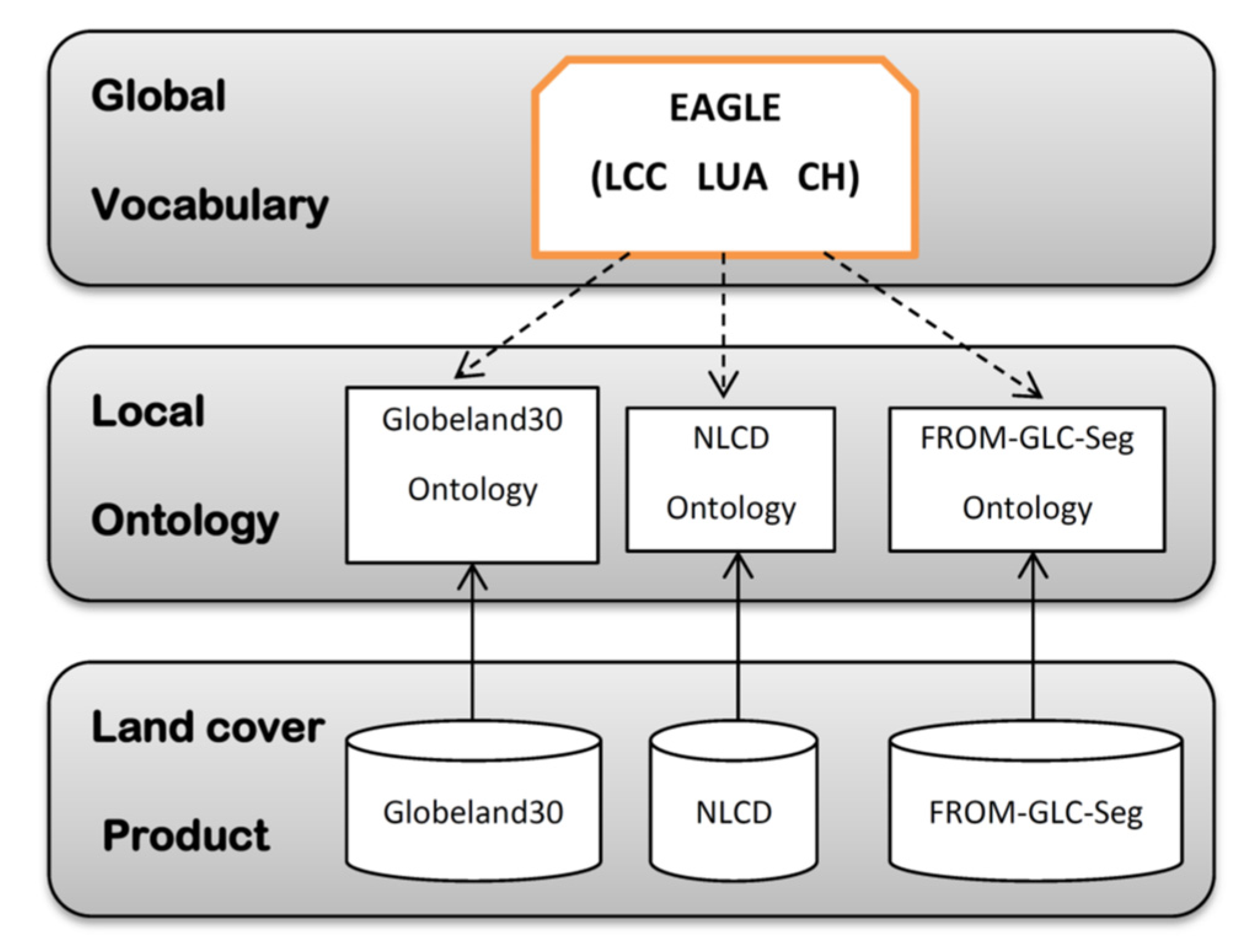
Figure 1. Ontology construction diagram. The black arrows represent transformation or access to the data, and the dotted arrows represent implicit relations.
Information 12 00236 g001
Figure 2. Three parts in the EAGLE Matrix: (a) land-cover components (LCCs); (b) land-use attributes (LUAs); (c) further characteristics (CH).
Information 12 00236 g002
Figure 3. Coniferous forest in the local ontology of FROM-GLC-Seg.
Information 12 00236 g003
Figure 4. GlobeLand30 land-cover ontology.
Information 12 00236 g004
Figure 5. NLCD2011 land-cover ontology.
Information 12 00236 g005
Figure 6. FROM-GLC-Seg land-cover ontology.
Information 12 00236 g006
Figure 7. Forest map in land-cover products: (a) GlobeLand30; (b) NLCD 2011; (c) FROM-GLC-Seg.
Information 12 00236 g007aInformation 12 00236 g007b
Figure 8. Verification points: (a) distribution of verification points of different sources; (b) distribution of verification points of different types; (c) randomly distributed visually interpreted sample points.
Information 12 00236 g008aInformation 12 00236 g008b
Figure 9. Local accuracy probability results: (a) NLCD2011; (b) FROM-GLC-Seg.
Information 12 00236 g009
Figure 10. Integration Model I: second-level class refinement results of GlobeLand30 forest.
Information 12 00236 g010
Figure 11. Integration Model II: second-level class refinement results of Globeland30 forest.
Information 12 00236 g011
Table 1. Similarity matrix.
Source Product Globeland30Broadleaf ForestConiferous ForestBroadleaf Coniferous Mixed Forest
NLCD2011deciduous forest S 11 N S 12 N S 13 N
evergreen forest S 21 N S 22 N S 23 N
deciduous evergreen mixed forest S 31 N S 32 N S 33 N
FROM-GLC-Segbroadleaf forest S 11 F S 12 F S 13 F
coniferous forest S 21 F S 22 F S 23 F
broadleaf coniferous mixed forest S 31 F S 32 F S 33 F
Table 2. Forest second level categories and definition of products.
Product NameFirst LevelSecond LevelDefinition
Globeland30ForestBroad-leaf forestThe forest with broadleaf tree species is built in groups, with a crown covering more than 30.0% of the land, and the height of the tree is more than 5 m high.
Coniferous forestThe general name of various forest plant communities composed of coniferous tree species, the crown coverage of more than 30.0% of the land, the height of the tree is more than 5 m.
Mixed forestConifers and broadleaf trees do not cover more than 60.0% of the total vegetation cover.
NLCD 2011ForestDeciduous forestAreas dominated by trees generally greater than 5 m tall, and greater than 20.0% of total vegetation cover. More than 75.0% of the tree species shed foliage simultaneously in response to seasonal change.
Evergreen forestAreas dominated by trees generally greater than 5 m tall, and greater than 20.0% of total vegetation cover. More than 75.0% of the tree species maintain their leaves all year. Canopy is never without green foliage.
Mixed forestAreas dominated by trees generally greater than 5 m tall, and greater than 20.0% of total vegetation cover. Neither deciduous nor evergreen species are greater than 75.0% of total tree cover.
FROM-GLC-SegForestBroadleafUsually higher reflectivity than conifer species in the near infrared (NIR) spectral band. Shaded and sunlit sides less contrast. Tree height is more than 5 m. Tree cover percentage is more than 15.0%. The crown density is more than 10.0%.
ConiferousLower reflectivity than broadleaf trees in the NIR band. Tree height is more than 5 m. Tree cover percentage is more than 15.0%. The crown density is more than 10.0%.
MixedNeither coniferous nor broadleaf trees dominate in a mixed forest stand. Tree height is more than 5 m. Tree cover percentage is more than 15.0%. The crown density is more than 10.0%.
Table 3. Change detection accuracy of pixel-based Landsat satellite imagery.
Category NameDefinitionStem Extraction Result
Broadleaf foresthaving relatively broad rather than needle like or scale like leaveswidth (broad) (01)leaf (01)forest (01)
Coniferous forestof or relating to or part of trees or shrubs bearing cones and evergreen leavespart (01)tree (01)shrub (01)cone (03)evergreen (01)leaf (01)forest (01)
Deciduous forestshedding foliage at the end of the growing seasonshedding (02)foliage (01)end (02)growing (01)season (02)forest (01)
Evergreen foresta plant having foliage that persists and remains green throughout the yearplant (02)foliage (01)green (01)year (01)forest (01)
Mixed forestComposition of mixed tree speciesblend (Mixed) (01)tree (01) forest (01)
Note: (01) and (02) represent the meaning interpretation order of the word in WordNet, because a word may have multiple meanings. When WordNet interprets the meaning of a word, it sorts each meaning. Different sorts represent different meanings, and the hierarchical relationship of the word in WordNet will change.
Table 4. Results of mapping based on term similarity.
Land Cover
Product
Globeland30Broadleaf ForestConiferous ForestBroadleaf Coniferous Mixed Forest
Source Product
definitionlexicalAveragedefinitionlexicalAveragedefinitionlexicalAverage
NLCD2011deciduous forest0.545 0.500 0.523 0.570 0.647 0.609 0.570 0.412 0.491
evergreen forest0.680 0.471 0.576 0.722 0.471 0.597 0.762 0.324 0.543
deciduous evergreen mixed forest0.540 0.313 0.427 0.576 0.344 0.460 0.657 0.471 0.564
FROM-GLC-Segbroadleaf forest1.000 1.000 1.000 0.788 0.412 0.600 1.000 0.500 0.750
coniferous forest0.655 0.412 0.534 1.000 1.000 1.000 1.000 0.500 0.750
broadleaf coniferous mixed forest0.685 0.500 0.593 0.867 0.500 0.684 1.000 1.000 1.000
Table 5. Results of mapping based on term similarity.
Land Cover Components (LCC)Land Use AtTributes/Function (LUA) Characteristics (CH)
Biotic/VegetationPrimary Production SectorSpatial PatternsLand Management(Bio-)Physical CharacteristicsGeneral Parameters
Woody VegetationForestryTexture PatternsForest Management TypeForest History TypeVegetation CharacteristicsHeight (m)Cover (%)
TreesShort rotationInterim or long rotationContinuous cover, selective loggingHomogenousMixed, heterogeneousMosaicScatteredIntensive monocultureRegularExtensive (selective logging)Endemic, primaryReforestationAfforestationLeaf formFoliage persistenceCrown cover density (%)Percentage of Ppecies (%) (Integer value)(Integer value)
Broadleaved treesNeedle-leaved treesPalm tree Coniferous/needle leavedBroad leavedEvergreenWinter deciduousSummer deciduous(Integer value)  (Integer value)
Table 6. Results of mapping based on attributes similarity.
Product Globeland30Broadleaf ForestConiferous ForestBroadleaf Coniferous Mixed Forest
Source Product
NLCD2011deciduous forest0.713 0.717 0.634
evergreen forest0.729 0.734 0.655
deciduous evergreen mixed forest0.635 0.640 0.791
FROM-GLC-Segbroadleaf forest0.892 0.866 0.809
coniferous forest0.858 0.892 0.809
broadleaf coniferous mixed forest0.783 0.802 0.975
Table 7. Result of similarity matrix of ontology mapping based on instance.
Source Product Globeland30Broadleaf ForestConiferous ForestBroadleaf Coniferous Mixed Forest
NLCD2011deciduous forest0.737 0.107 0.082
evergreen forest0.450 0.390 0.096
deciduous evergreen mixed forest0.455 0.140 0.300
FROM-GLC-Segbroadleaf forest0.639 0.077 0.060
coniferous forest0.215 0.597 0.010
broadleaf coniferous mixed forest0.297 0.154 0.505
Table 8. Comprehensive mapping result.
Product Name Globeland30Broadleaf ForestConiferous ForestBroadleaf Coniferous Mixed Forest
Source Data
NLCD2011deciduous forest0.657 0.478 0.402
evergreen forest0.585 0.573 0.431
deciduous evergreen mixed forest0.506 0.413 0.552
FROM-GLC-Segbroadleaf forest0.844 0.514 0.540
coniferous forest0.535 0.830 0.523
broadleaf coniferous mixed forest0.558 0.547 0.827
Table 9. Accuracy evaluation matrix of integration results based on Model I.
TypeOverall AccuracyUser AccuracyCommission
Error
Omission
Error
Producer
Accuracy
Broadleaf 0.826 0.174 0.160 0.840
Coniferous 0.720 0.280 0.098 0.902
Mixed 0.483 0.517 0.216 0.784
Sum0.753
Table 10. Accuracy evaluation matrix of integration results based on Model II.
TypeOverall AccuracyUser AccuracyCommission
Error
Omission
Error
Producer
Accuracy
Broadleaf 0.826 0.174 0.148 0.852
Coniferous 0.720 0.280 0.084 0.916
Mixed 0.600 0.400 0.122 0.878
Sum0.763
Publisher’s Note: MDPI stays neutral with regard to jurisdictional claims in published maps and institutional affiliations.