Popularity Prediction of Instagram Posts

Abstract

Predicting the popularity of posts on social networks has taken on significant importance in recent years, and several social media management tools now offer solutions to improve and optimize the quality of published content and to enhance the attractiveness of companies and organizations. Scientific research has recently moved in this direction, with the aim of exploiting advanced techniques such as machine learning, deep learning, natural language processing, etc., to support such tools. In light of the above, in this work we aim to address the challenge of predicting the popularity of a future post on Instagram, by defining the problem as a classification task and by proposing an original approach based on Gradient Boosting and feature engineering, which led us to promising experimental results. The proposed approach exploits big data technologies for scalability and efficiency, and it is general enough to be applied to other social media as well.

1. Introduction

Presently, the social network market grows both in number of operators and in number of posts, exponentially. With millions of monthly active users, both on mobile devices and web browsers, Instagram represents a leading platform in this market. Launched in 2010, it has gradually gained a leading role among photo-sharing platforms, introducing several innovative features over times, including—not exhaustively—filters, stories, and an internal messaging system. Recently, these features have attracted not only ordinary users and photography enthusiasts, but also companies, organizations and global brands, thanks to the possibility that Instagram has offered to explore new business models and marketing strategies.

In such a context, approaches aimed to predict the popularity of social content are gaining increasing attention, not only from a commercial and industrial standpoint, but also from a scientific perspective. Indeed, thanks to the advancement of knowledge in the fields of data analysis and artificial intelligence, together with the development of new techniques based on Machine/Deep learning, Reinforcement Learning, Natural Language Processing (NLP), Data mining, Big Data, etc. [1,2,3,4,5,6,7], it is now possible to provide advanced tools for companies and individuals, and promote the consolidation of these businesses in the social market. For this purpose, such tools and techniques usually aim to extract hidden information that may be exploited in several directions, spanning from targeted advertisements to political strategies.

Within this context, the present work proposes a novel approach for predicting the future popularity of Instagram posts. In particular, the existing literature often focuses on the prediction of the so-called engagement factor (i.e., the ratio between expected likes and number of followers of the account), thus addressing a regression problem. Conversely, this paper aims to determine whether, for the post to be published, the deviation from the average number of likes of recent posts will be positive or negative, therefore solving a binary classification task. More precisely, our method predicts the expected popularity class regardless of the selected media (image or video), which we assume as fixed by the user: vice versa, we analyze the metadata associated with the post (e.g., the caption, the chosen hashtags, the expected time and date of publication, the used emojis), as well as the additional information related to the account and the popularity of recent posts.

Therefore, the main contributions of this work are:

• an original formulation of the problem to address, by defining it as a binary classification task, with the aim of determining whether the popularity of a future post will increase or decrease compared to the average popularity value of the past posts;
• a novel approach based on feature engineering and machine-learning techniques for the prediction of the expected popularity class of posts on Instagram (although the approach is general and applicable to other social networks);
• an experimental evaluation of the approach, comparing the results against a set of strong baselines, in different scenarios (obtained through an extensive exploration of the problem parameters);
• a big data infrastructure that we have leveraged to run the proposed approach and that makes it scalable and flexible;
• an analysis of the execution performance of the proposed algorithm, by considering a distributed cloud deployment, and by exploiting the aforementioned big data infrastructure.

The remainder of this paper is then organized as it follows. In Section 2, we present some background notions related to the adopted machine-learning techniques, and a wide overview of the related work. Then, in Section 3 we outline the problem to be addressed and describe it in a formal way. Section 4 contains the procedure adopted for collecting the data and building the dataset, whereas in Section 5 we describe in detail the proposed approach. Finally, in Section 6 we illustrate the results of the experimental evaluation, and in Section 7 we conclude the work, indicating some possible future developments.

2. Background and Related Work

This section provides a background on the techniques and methods exploited in this work, along with an overview and some representative examples of state-of-the-art works focused on this research field.

2.1. Machine-Learning Algorithms

On the basis of the target strategy, the type of involved input/output data, and the type of problem to face, the existing literature proposes several types of machine-learning algorithms (e.g., supervised learning, unsupervised learning, semi-supervised learning, reinforcement learning, self-learning, feature learning, etc.). However, the most adopted classification essentially comprises three main groups: supervised, unsupervised, and semi-supervised [8,9].

Intuitively, in the supervised case, the learning is achieved by leveraging on a previous knowledge of the possible output value for each sample. The objective is hence to learn a function able to approximate the relationship between the input and the output. More formally, given an instance space X and a label space Y, let us suppose there exists a target function $y=f\left(x\right)$, with $x\in X$ and $y\in Y$, able to map each x to the correct y: the supervised algorithm tries to generalize the function $f\left(x\right)$, by observing a (possibly large) set of $(x,y)$ sample pairs. Supervised learning can thus address both regression [10] and classification [11] problems: the first case, when the output variable y is numerical (or continuous); the second case, when the output variable y is categorical (or discrete). For these reasons, supervised algorithms have been widely exploited in the literature: some examples are represented by Random Forests [12], Support Vector Machines [13], Gradient Boosting [14], Neural Networks [15].

On the other hand, in the unsupervised learning, labeled outputs are not necessary for the training phase. Indeed, unsupervised algorithms try to detect some hidden patterns on the input data, in order to find a structure in them. They are mainly grouped in clustering algorithms [16] (that aggregate data into similar sets, according to one or more defined metrics) and association algorithms [17] (that search for rules able to describe large portions of the given data). The two most common techniques, in this category, are the K-means [18] for clustering tasks, and the Apriori [19] for association tasks.

Finally, as previously mentioned, there exists also a third approach, defined semi-supervised [9] learning, which represents a combination of the supervised and unsupervised approaches: here, a small part of the labeled samples is used for the training stage, to facilitate the learning of the remaining large amount of unlabeled input data.

2.2. Ensemble Learning

With the expression ensemble learning, literature usually refers to a machine-learning paradigm that exploits multiple models, i.e., the weak learners, which are trained and combined together in order to solve specific problems. Indeed, this strategy relies on the idea that such a combination of several single (weak) models, in particular if associated with a proper feature selection step [20], can lead to an improvement of the final accuracy.

In this context, a machine-learning technique able to face both regression and classification tasks, effectively, is the aforementioned Gradient Boosting [14]: here, a model is created in a gradual, additive, and sequential way, and it is generalized by allowing the optimization of an arbitrary differentiable loss function [21]. On the other side, a second well-known algorithm, based on the same ensemble learning paradigm, and that is widely used in the literature thanks to its performance, is represented by the previously mentioned Random Forests [12]. It exploits the same Gradient Boosting mechanism to build the prediction model. Specifically, it uses a large number of single decision trees, which operate in an ensemble way. Each single tree outputs a class prediction, and the final prediction of the model is given by the class with the most votes.

For these reasons, in this work we exploit both Gradient Boosting and Random Forest-based techniques in order to build our general algorithm for predicting the popularity class of Instagram posts, as better explained in Section 5. In particular, the former is used as the main method, whereas the latter represents a variant used for the comparison. The adopted paradigm is therefore a supervised one and, specifically, the ensemble learning described above.

2.3. Popularity in Social Media

Several literature approaches have recently emerged on this topic, proposing different strategies in terms of data collection, method of classification, and measure of popularity used. For example, Gayberi et al. [22], in their proposal, exploit a tailor-made dataset of 210,630 posts extracted from common Instagram accounts, enriched with several features related to posts, user profiles, images and statistical features, addressing the problem as a regression task. Experiments have been performed using different machine-learning algorithms, from Random Forest to MLP and Deep Learning, comparing the results in terms of MAE and RMSE. De et al. [23] analyze 1280 Instagram posts from Indian users, trying to predict the popularity score as a range of achieved likes, grouped by 25 (e.g., 0–25, 25–50, etc.). Their solution, based on a Deep Learning approach, leverages the type of filter applied to the image, the location, the day of the week and time of posting, the caption, the number of users tagged, and the hashtag list.

Other studies have been also conducted in different social contexts such as, for instance, Twitter, where in [24] the authors propose a study aimed at the prediction of the tweet popularity as a classification problem. Similarly, in [25], a sentiment analysis task has been performed on the Twitter posts, in order to measure the positive or negative influence of popular users. In this direction, the prediction of the retweet rate of a given tweet has been also investigated in [26], whereas a micro-prediction model aimed at evaluating the Twitter message propagation for a user has been proposed in [27].

A study focused on the analysis and prediction of the news popularity in Telegram has then been performed in [28], where the authors underline the differences between the definition of a popularity score in such a platform, with respect to other social media. In [29], the authors propose a regression method to predict the online video popularity based on the number of views, by taking into account YouTube and Facebook platforms. Specifically, the literature shows how the exploitation of information from social media becomes increasingly important. In [30], such an information has been exploited in order to predict e-commerce products prices, whereas in [31] the authors performed an evaluation of products and services through unsolicited social contents. Similar research work has instead focused on group identification and recommendation in social networks: for instance, in [32], Alduaiji et al. propose an influence propagation model for community detection, to identify and understand user relationships in social media, while in [33], Carta et al. present a novel method for the prediction of the ratings in a social group recommendation scenario in which groups are detected by clustering the users.

On the other side, many studies are instead oriented to a deeper analysis of the social media posts, such as in [34,35], where the authors propose approaches for toxic comment classification. Indeed, similarly to other contexts [36,37,38,39,40,41,42], a considerable importance is given to the transformation of the original data domain, such as, for instance, in [43], where an approach aimed to predict the popularity of online videos by exploiting the Fourier transform has been presented. Another example is represented by the work in [44], where the authors propose a solution based on the wavelet transform to detect human, legitimate bot, and malicious bot in online social networks. However, as it happens in related fields [45], the preferences of the users over time could be biased by several factors, not reflecting their real preferences [46]. A systematic overview has been provided in [47], where the authors reviewed the recent literature, offering statistics and discussing about methods, algorithms, techniques, and challenges.

3. Problem Formulation

Differently from other literature works, which commonly formulate the problem as a regression task, with the goal of estimating the so-called engagement factor (i.e., the ratio between expected likes over account followers) of a future post, we model the problem as a binary classification task.

More specifically, our goal is to determine if a future Instagram post will be popular or unpopular, regardless of the type of visual content published (image or video), but mainly focusing on the post metadata such as the caption, the time of publication, and the account typology. In particular, we label as popular a post whose number of (expected) likes will exceed a specified threshold (roughly, the moving average of likes of the account), or as unpopular otherwise.

To formalize this concept, we first need to introduce the preliminary definition of the Likes Moving Average (LMA). Intuitively, given the i-th post of an Instagram account, the LMA represents the average number of likes achieved by its previous K posts. In formulae, let ${\mathbf{P}}_A$ be the ordered set of posts published by an account A; then, we have:

$$LM{A}_K(i,A)=\frac{{\sum }_{j=i-K}^{i-1}\mathtt{like}\_\mathtt{count}\left({\mathbf{P}}_A\left[j\right]\right)}{K}$$

(1)

where K is the number of previous posts considered (i.e., the size of the moving average window), and $\mathtt{like}\_\mathtt{count}\left({\mathbf{P}}_A\left[j\right]\right)$ is the number of likes obtained by the j-th post of A (To simplify our model, we assume to collect the number of likes of a given post, only after this value has stabilized over time and will not vary significantly in the future).

Given $LM{A}_K$, we can now derive the Popularity Class (PC) associated with the i-th post of the account A, as it follows:

$$P{C}_{K,\Delta }(i,A)=\left\{\begin{array}{cc}1\mathrm{or}popular,\hfill & \mathrm{if}\mathtt{like}\_\mathtt{count}\left({\mathbf{P}}_A\left[i\right]\right)>(1+\Delta )·LM{A}_K(i,A)\mathrm{or}\hfill \\ 0\mathrm{or}unpopular,\hfill & \mathrm{otherwise}.\hfill \end{array}\right.$$

(2)

that when the parameter $\Delta =0$, essentially defines as popular a post i of A, if its expected number of likes is greater than the average likes of the previous K posts (i.e., $LM{A}_K$). In this context, $\Delta$ represents a tolerance threshold for the definition of popular posts: for instance, given $\Delta =0.2$ and $K=50$, a post is labeled as popular if its achieved likes are greater or equal than $20\%$ of the average likes of its preceding 50 posts.

4. Data Collection

In this section, we describe in detail the process adopted to build the dataset used for the study and testing of our approach.

Although some Instagram datasets already exist in the literature or are available on the web, we opted to build a new one from scratch. This choice was essentially driven by two reasons: (i) the social network sector is constantly evolving, and sees a steady emergence of new features, different recommendation policies, and explosive growth in content, therefore databases generated a few years earlier may not fully reflect the current situation; and, (ii) for the type of analysis to be performed, we needed a large dataset, with raw and genuine contents, and the widest possible set of features.

To build the dataset, we first collected a preliminary list of Instagram account identifiers, from which the full posts are extracted. The steps required for this process are depicted in Figure 1: starting from the preliminary list of accounts, we exploited a browser extension (https://instagramhelpertools.com/) for Google Chrome to export—for each of them—the full list of followers. Therefore, we iteratively extended the list of accounts, until a sufficiently large number of accounts was reached. Then, we leveraged our software module, developed in Python, to remove duplicates and filter accounts according to the following specifications: first, we selected ordinary profiles only (i.e., those with less than 25,000 followers); second, we required that each selected account has at least 100 published posts; and, third, we discarded accounts with private visibility.

Once we completed this step, and we have then obtained the final list of accounts on which to build the dataset, we used our same Python module to interface with Instagram, through integration with an open-source crawler (https://github.com/huaying/instagram-crawler). In this way, we proceeded to the extraction, on average, of the last 100 posts of each collected user; in particular, the list of complete posts of each account (along with some general profile information) has been separately stored on disk, organized in an appropriate directory as a json file.

As already mentioned, although we also stored the URL of the visual content related to the post (i.e., the image or video) into the final json document, this content is not taken into account by this work (it is stored for possible future purposes, see Section 7), which instead aims to determine the popularity of a future post of Instagram according to the metadata chosen (caption, publication time, hashtags, etc.), thus assuming that the visual content itself is predetermined and not amendable. Hence, following this scheme, we collected the post and profile features described in

Table 1. Dataset features collected from Instagram.

Feature	Description
is_video	A binary feature that indicates if the post content is an image or a video.
likes_num	The number of likes received by the post.
timestamp	The publication date and time of the post.
followers_num	The number of followers of the post author.
caption	The full caption of the post, including emojis and hashtags.

.

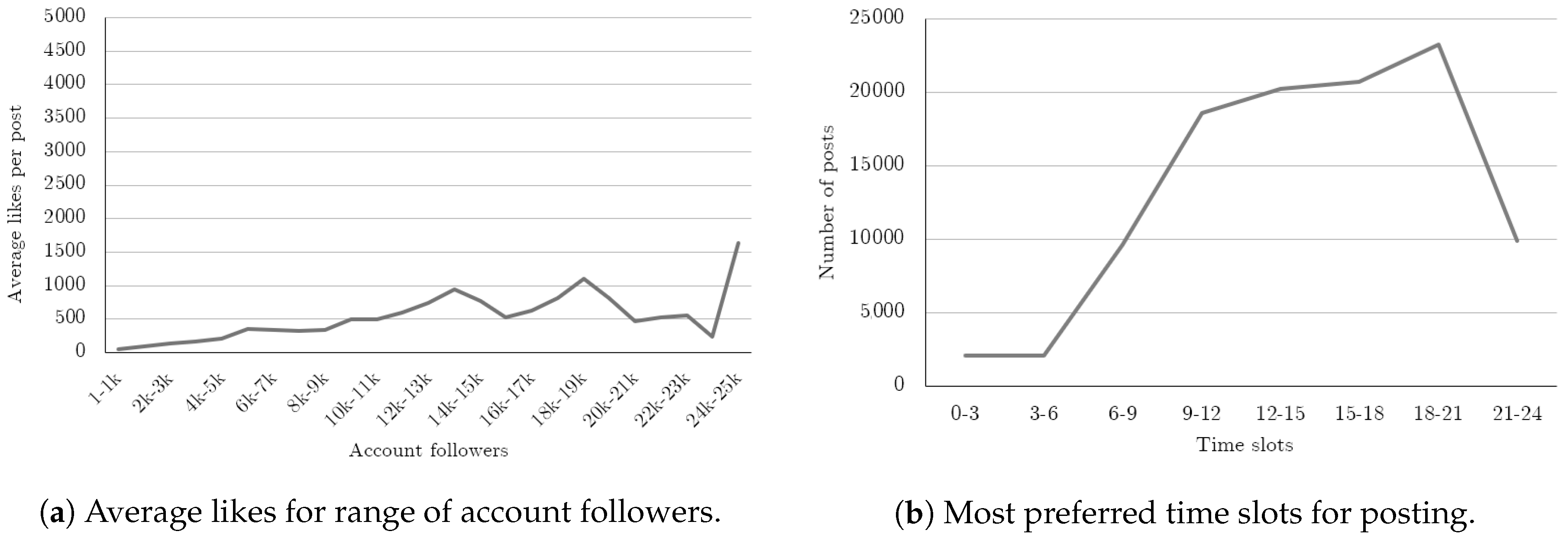
Overall, the final dataset we collected thus consists of 106,404 rows, for a total of 2545 different users. On average, each user has 2071 followers. Finally, in Figure 2, we show some statistics related to the considered accounts: in particular, the sub-figure (a) shows that the average of achieved likes per post is, in proportion to the followers, higher for smaller accounts, whereas (b) outlines the typical publication times chosen by these accounts, in which the 18:00–21:00 time range appears to be the most popular one.

5. Proposed Method

In this section, we now describe the proposed method to address the problem of predicting the popularity class of a future Instagram post (as defined in Section 3), through a supervised learning technique and by exploiting user-generated metadata (caption, hashtag, publication time, etc.) as features. As previously mentioned, our method does not perform any kind of analysis on the type of visual content that the user intends to publish (picture or video), since the goal is to verify whether the background information generated by the user is useful to promote the aforementioned content, or, vice versa, whether it may penalize the expected popularity. Moreover, such a consideration allows us to generalize our approach and apply it to other social networks where only text is reported.

In particular, the proposed method that we named XGBoost Instagram Predictor (XGB-IP), consists of two main steps:

• a feature engineering phase, in which, starting from the fetched data (according to the procedure described in Section 4), we enriched the dataset with some derived information, as well as removing data whose contribution was negligible or not interesting for the class prediction purposes;
• a supervised learning step, where the classification model is built on the features obtained from the step (1), and then used for the popularity class prediction of new posts.

An overview of the proposed approach is then outlined in Figure 3, whereas its details are described below.

5.1. Feature Engineering

Starting from the data collected as described in Section 4, we performed a feature engineering stage, where we enriched the dataset with several additional features, in order to boost the performance of the classifiers and to improve the overall accuracy of the approach.

A first set of features provides some indicators related to the last posts published by the account in question. Then, a second set of features is derived by processing the chosen caption of the future post, as well as the expected timestamp of publication. A summary of these extra features is provided in

Table 2. Advanced features generated by processing the collected input data.

Feature Type	Description
Average likes	Average number of likes of the K most recent posts of the account, for different values of K.
Recent likes	The exact number of likes achieved by the most recent published posts.
Time features	The scheduled date and time of the post to be published.
Text-related features	The features derived from the caption (number of words, sentiment score, hashtags popularity, emoji, etc.).

.

First, we considered the average likes achieved by the K most recent posts published by the account. This information in fact provides an effective indicator for estimating an account popularity trend, and has also been exploited to define the baselines used as a comparison in Section 6. In this regard, we extended the dataset with a column for each $K\in \{5,10,15,20,30,50\}$. Then, we introduced a few more targeted features, providing the exact number of likes of the latest published posts. To this purpose, we only considered the last 5 previous posts because, from preliminary analysis, we observed that data from older posts had a negligible impact on the accuracy results (since their information was well absorbed by the averages).

We therefore transformed the data related to the scheduled time and date of publication into separate features, specifying the time, day of the week, month and season of planned publication.

Finally, as a last but not less important step, we analyzed the caption of the posts, extracting the number of words, the number of users tagged, the number (and importance) of chosen hashtags, and, notably, a sentiment score [48,49,50], calculated using the SentiStrength library (http://sentistrength.wlv.ac.uk/), after filtering hashtags and mentions. We also paid particular attention to the presence of emojis in the caption. Hence, we defined 10 macro-categories, corresponding to 10 different features/columns: happiness, love, sadness, travel, food, pet, angry, music, party and sport. Each of these represents a binary feature, whose value depends on the presence, in the caption, of at least one emoji which is relevant to the category (note that the set of categories has been reduced as a result of preliminary empirical testing; similarly, the use of binary features has shown to be more effective than the use of discrete features which also count the number of emojis present in the text).

In parallel, we also collected all the hashtags referred in the posts of our dataset, and then we associated a weight to each of them, intended as the number of posts in which they appear, relative to the whole Instagram network. Then, similarly to what we did for the emojis, we created 10 macro-categories of hashtags, corresponding to 10 different levels of hashtag popularity (determined by dividing into 10 parts the range of weights between the most used and the least used hashtag, according to logarithmic scale). In this way, each macro-category corresponds to a binary feature that is set to 1 when the caption includes at least one hashtag which belongs to that level.

Finally, we added the popularity class (PC) to the dataset (to be used for the training stage), represented by a binary label that assumes the value 1 if the considered post is popular, and 0 otherwise (according to the definition mentioned in Section 3). Specifically, we added a separated label for each different pair of parameters K and $\Delta$ (with K indicating the number of previous posts taken into account, and $\Delta$ the tolerance threshold for the classification of the future post as popular). In particular, for our experimental scenarios, described in Section 6, we consider K values equal to 10, 30 and 50, while $\Delta$ values equal to 0, 0.05, 0.1 and 0.15.

5.2. Supervised Learning

The key contribution of the proposed approach lies in the exploitation of supervised learning techniques that, through the training of classification tools using the labeled input data from our dataset, generate the appropriate models for the prediction of the expected popularity of future posts. For this purpose, as a result of preliminary tests and also depending on the type of data processed, the choice has fallen mainly on the XGBoost algorithm (which represents an efficient implementation of the previously mentioned Gradient Boosting). We called the overall method XGBoost Instagram Predictor (hereafter, XGB-IP). However, for the classification phase, we also implemented a variant based on the Random Forest algorithm, as a further point of comparison. Similarly, this variant has been named Random Forest–Instagram Predictor (hereafter, RF-IP).

We tested the classification algorithms with different configurations, by performing a parameters exploration, mainly on the following: learning_rate, which represents the shrinkage of each tree contribution; n_estimators, which is the number of boosting stages to perform; and max_depth, which represents a limitation of the number of nodes in each tree.

Table 3. Algorithm parameters.

Algorithm	Parameters
XGBoost–Instagram Predictor (XGB-IP)	learning_rate	0.1
	n_estimators	750
	max_depth	5
Random Forest–Instagram Predictor (RF-IP)	n_estimators	750
	max_depth	5

shows the final obtained configurations, for both the classification algorithms considered. In addition to those mentioned above, several tests were also performed on the other parameters. However, since they did not bring significant improvements in accuracy or execution time, we opted to use the default values.

Once the parameters are defined, the supervised learning is then performed in two stages: (i) by fetching the input data (from the enriched dataset), to build the appropriate training and test sets; (ii) by training the classifier. Finally, the prediction module, which integrates the output model, is made accessible either as a software API or through a facilitated user interface.

6. Experimental Evaluation

In what follows, we illustrate the experiments we carried out to validate the effectiveness of our method, performed by considering the dataset described in Section 4.

6.1. Implementation Details

Before going into the details of the conducted experiments, we first introduce the distributed architecture and the associated implementation details, used for the construction of the dataset and for the execution of the experiments described below.

With respect to the creation of the dataset (i.e., the collection of the list of Instagram accounts, the download of all the posts data, etc.), we exploited a typical laptop, running Microsoft Windows 10. Conversely, for the training phase, we opted for a distributed implementation, in order to evaluate the scalability of the approach and to exploit big data technologies and tools. To this purpose, we leveraged on the following software:

• the Amazon AWS / EC2 cloud computing platform (https://aws.amazon.com/it/ec2/), to build the cluster infrastructure used for our experiments;
• the HashiCorp Terraform tool (https://www.terraform.io/), for the management and provisioning of the AWS instances;
• the Apache Spark framework (https://spark.apache.org/), for the distributed computing, in particular its Python wrapper XGBoost4J-Spark (https://xgboost.readthedocs.io/en/latest/jvm/xgboost4j_spark_tutorial.html), which allowed us to integrate Spark and XGBoost;
• the Apache Hadoop framework (https://hadoop.apache.org/), to handle the dataset.

Through these tools, we set up different distributed clusters, consisting of 1, 2, 4 and 8 parallel workers respectively, to compare their performance. In this context, each worker corresponds to a t2.medium AWS instance, each one featuring the following technical specifications:

• Operating System: Ubuntu Server 18.04 LTS;
• Processor: Intel Xeon (up to 3.3 GHz);
• vCPU (#): 2;
• Memory (GB): 4.

Table 4. Execution time of a single iteration as cluster size increases (each Apache Spark worker runs on a separate machine).

Workers	Instance Type	Execution Time
1	t2.medium	55.59 s
2	t2.medium	51.75 s
4	t2.medium	48.15 s
8	t2.medium	40.25 s

shows the execution times of the training phase, in seconds, as the cluster size increases. We observe how the exploitation of the big data management tools, as well as a parallel architecture for running the training phase, allowed us to obtain a significant time saving of ∼38% in terms of execution performance, when a cluster size consisting of 8 workers was used (compared to the use of a single machine).

This result makes it possible to affirm that the distributed implementation of the method is adequately scalable, and can be therefore extended in order to exploit a much larger dataset (with millions of posts) and a possibly larger number of features.

6.2. Monte Carlo Cross-Validation

The experiments were carried out on the entire dataset, by exploiting the Repeated hold-out validation technique, also known as Monte Carlo cross-validation [51]. Compared to the K-fold approach, although both methods achieve the statistical significance of the result, Monte Carlo allows exploration of a larger number of partitions of the dataset, providing a more accurate estimate of the real accuracy of the algorithm (as it reduces the variance), in order to decrease the risk of overfitting.

To this end, we performed multiple independent runs, each with random partitioning of the dataset in a training set with the 90% of the samples, and a test set with the remaining 10% of the samples. Moreover, the split between train and test is performed without replacement, and with stratification, i.e., ensuring that the distribution of the classes of the full dataset is preserved in the individual sets.

6.3. Baselines

To better evaluate the effectiveness of the proposed method, as well as to highlight the contribution of the used feature engineering and supervised learning techniques, we now provide a set of baselines for the comparison of the results.

There are three primary baselines and a fourth obtained as the average of the three. They are not based on machine-learning techniques. The idea behind these baselines lies in the assumption that future posts to be published reflect the performance of the most recent posts: informally, for each of first three of them, the expected class of popularity of the future post is defined as the class (already known a priori) of—respectively—the most recent, second most recent and third most recent post already published by the same Instagram user.

In formulae (by recalling the definition of Popularity Class from Equation (2)):

$$Baselin{e}_j\_P{C}_{K,\Delta }(i,A)=P{C}_{K,\Delta }(i-j,A),\mathrm{with}0<j\le 3$$

(3)

We also observe that although these baselines globally obtain good performance (especially as the value of the considered K parameter increases), the best one is given by fixing $j=1$ (Baseline 1); in particular, for values of $j>3$, we found a rapid decay of the baseline accuracy. Therefore, hereafter, we only consider $j\in \{1,2,3\}$ for our comparison.

However, we introduce an additional baseline, which represents a special case, and we indicate it with index $j=4$ (Baseline 4). It is simply defined as the average of the first three baselines:

$$Baselin{e}_4\_P{C}_{K,\Delta }(i,A)=\frac{\sum _{j=1}^{3}P{C}_{K,\Delta }(i-j,A)}{3}$$

(4)

The baselines defined above will then be used in the remainder of this section for the comparison with the proposed method.

6.4. Evaluation Metrics

Before proceeding with the presentation of the experimental results, let us illustrate the metrics we considered for the assessment of our approach.

6.4.1. Accuracy

This metric gives us information about the number of instances correctly classified, compared to the total number of them. It provides an overview of the performances of the classification. Formally, given a set of X Instagram posts on which to make a popularity prediction, the accuracy is calculated as shown in the following equation, where $\left|X\right|$ stands for the number of posts and $X^{(+)}$ stands for those correctly classified.

$$Accuracy\left(X\right)=\frac{X^{(+)}}{\left|X\right|}=\frac{tp+tn}{tp+tn+fp+fn}$$

(5)

where tp represents the number of true positives, tn the number of true negatives, fp the number of false positives and fn the number of false negatives.

6.4.2. Balanced Accuracy

This is a suitable metric for evaluating how good a binary classifier is, especially when the classes are unbalanced. It is defined as the average of recall obtained on each class. The recall metric $R_c$ for a generic class can be defined as follows:

$$R_c=\frac{tp}{(tp+fn)}$$

(6)

Using this definition, we can obtain the balanced accuracy in the following way:

$$\frac{R_{c0}+R_{c1}}{2}$$

(7)

where R${}_{c0}$ and R${}_{c1}$ represent, respectively, the recall value for class 0 (unpopular) and class 1 (popular), respectively.

6.4.3. F1-Score

The F1-Score is a weighted average of two metrics: precision and recall. Recall metric $R_c$ is calculated as defined in Equation (6). Similarly, we define the precision $P_c$ for a generic class:

$$P_c=\frac{tp}{(tp+fp)}$$

(8)

with tp representing the number of true positives and fp the number of false positives. Based on Equations (6) and (8) we can then define F1-Score $F_c$, for a generic class c, as:

$$F{1}_c=2\times \frac{P_c\times R_c}{P_c+R_c}$$

(9)

This metric is calculated independently for each of the two classes $c0$ and $c1$, resulting in two values $F{1}_{c0}$ and $F{1}_{c1}$. At this point, the final result is obtained as follows:

$$weighte{d}_{F1}=F{1}_{c0}\times W_0+F{1}_{c1}\times W_1$$

(10)

with $W_0$ and $W_1$ representing the weights associated with the two classes, whose values depend on the number of true instances of each class.

6.5. Results

We now show the results of the experimental evaluation of our algorithm, in terms of the metrics described in Section 6.4, and by comparing it with the baselines outlined above.

We performed a total of 12 experiments, by spanning different combinations of K (10, 30 and 50), i.e., the number of previous posts used to calculate the recent average of likes, and different values of $\Delta$ (0, 0.05, 0.1 and 0.15), i.e., the minimum positive deviation from the average to classify the future post as popular. As an example, if we consider $K=30$ and $\Delta =0.05$, a post will be classified as popular, if its number of expected likes will be at least $5\%$ higher than the average likes of the last 30 posts of that user.

Specifically,

Table 5. Results of the experiments for $K=10$ (best values are highlighted in bold).

	$\mathit{K}=10$
	$\Delta =\mathbf{0}$			$\Delta =\mathbf{0.05}$
	Accuracy	Balanced Accuracy	F1-Score	Accuracy	Balanced Accuracy	F1-Score
Baseline 1	52.86%	52.69%	52.86%	53.92%	52.53%	53.83%
Baseline 2	51.05%	50.83%	51.02%	52.06%	50.49%	51.89%
Baseline 3	49.92%	49.68%	49.89%	51.44%	49.77%	51.22%
Baseline 4	52.51%	52.56%	52.56%	54.15%	52.61%	53.98%
RF-IP	55.12%	53.23%	49.76%	58.60%	51.11%	45.82%
XGB-IP	57.63%	57.22%	57.42%	59.59%	55.63%	56.86%
	$\Delta =\mathbf{0.1}$			$\Delta =\mathbf{0.15}$
Baseline 1	56.21%	52.65%	55.94%	58.91%	52.61%	58.43%
Baseline 2	54.28%	50.41%	53.90%	57.45%	50.69%	56.80%
Baseline 3	53.94%	49.85%	53.45%	57.19%	50.13%	56.39%
Baseline 4	57.56%	52.81%	56.53%	61.61%	52.84%	59.48%
RF-IP	62.86%	50.38%	49.18%	66.95%	50.34%	54.16%
XGB-IP	63.10%	53.97%	57.17%	67.13%	53.13%	59.30%

shows the results for $K=10$ and all the considered thresholds $\Delta$. This is the worst-case scenario, since the prediction of the post popularity takes into account the average likes of the 10 most recent posts only, thus examining a short-term trend. Focusing on the competitors, we observe that the best baseline is the #4, although for $\Delta =0$, the baseline 1 reaches slightly better results. In this context, our method (XGB-IP) gets the best overall performance for all the $\Delta$ thresholds (except for the F1-Score with $\Delta =0.15$). Here, the most significant value is a 57.22% of balanced accuracy for $\Delta =0$: in this case, we get a relative improvement of +8.59% compared to the best baseline, as well as a +7.46% compared to the Random Forest variant of our method. This gap decreases as $\Delta$ grows; for $\Delta =0.15$, in fact, the performance is very similar to that of the competitors. A possible explanation for this behavior lies in the fact that posts that achieve a high increase in popularity compared to the account recent average are very unusual or characterized by deeper semantic peculiarities, and therefore difficult to predict by classification models that exploit the features of the proposed approach.

By moving to $K=30$ (

Table 6. Results of the experiments for $K=30$ (best values are highlighted in bold).

	$\mathit{K}=30$
	$\Delta =\mathbf{0}$			$\Delta =\mathbf{0.05}$
	Accuracy	Balanced Accuracy	F1-Score	Accuracy	Balanced Accuracy	F1-Score
Baseline 1	56.78%	56.77%	56.79%	57.09%	56.51%	57.08%
Baseline 2	55.65%	55.64%	55.65%	55.95%	55.29%	55.91%
Baseline 3	54.29%	54.26%	54.29%	54.94%	54.21%	54.87%
Baseline 4	58.14%	58.21%	58.11%	58.37%	57.94%	58.41%
RF-IP	59.22%	59.20%	59.22%	59.97%	57.78%	58.33%
XGB-IP	61.17%	61.19%	61.17%	61.92%	60.49%	61.30%
	$\Delta =\mathbf{0.1}$			$\Delta =\mathbf{0.15}$
Baseline 1	58.65%	56.72%	58.59%	60.34%	56.52%	60.19%
Baseline 2	57.28%	55.19%	57.17%	58.97%	54.84%	58.73%
Baseline 3	56.54%	54.27%	56.36%	58.88%	54.54%	58.55%
Baseline 4	60.21%	58.18%	60.08%	62.46%	58.00%	61.95%
RF-IP	62.52%	55.05%	56.10%	64.98%	51.77%	53.68%
XGB-IP	64.09%	59.22%	61.77%	66.70%	57.81%	62.70%

), i.e., by increasing the number of recent posts considered, all methods considered get better results. However, our approach is confirmed as the best, with the exception—also in this case—of $\Delta =0.15$ (but with a result still comparable to that of baseline 4). The balanced accuracy for $\Delta =0$ is 61.19%, with a relative increase of +5.12% compared to baseline 4. We also note that for this configuration, even the variant based on Random Forest obtains a good result, but it worsens dramatically as $\Delta$ increases.

Finally, for $K=50$, our method obtains the best overall result, with a balanced accuracy of 64.72% for $\Delta =0$ (in relative terms, it means a +5.03% if compared to the best baseline, and a +3.9% if compared to the Random Forest variant), hence achieving a good predictivity.

Moreover, in this last setup, besides clearly overcoming all the competitors, the result of our method for $\Delta =0.15$ (i.e., the ability to predict whether the considered post will reach several likes more than 15% higher than the average of the last 50 published ones) has shown to be particularly significant. Indeed, as illustrated in

Table 7. Results of the experiments for $K=50$ (best values are highlighted in bold).

	$\mathit{K}=50$
	$\Delta =\mathbf{0}$			$\Delta =\mathbf{0.05}$
	Accuracy	Balanced Accuracy	F1-Score	Accuracy	Balanced Accuracy	F1-Score
Baseline 1	59.57%	59.54%	59.57%	59.91%	59.73%	59.90%
Baseline 2	58.74%	58.72%	58.74%	58.82%	58.63%	58.81%
Baseline 3	57.51%	57.49%	57.51%	57.77%	57.53%	57.74%
Baseline 4	61.75%	61.62%	61.64%	61.80%	61.78%	61.84%
RF-IP	62.39%	62.29%	62.33%	62.64%	62.29%	62.53%
XGB-IP	64.82%	64.72%	64.76%	64.95%	64.57%	64.83%
	$\Delta =\mathbf{0.1}$			$\Delta =\mathbf{0.15}$
Baseline 1	60.51%	59.59%	60.49%	61.71%	59.51%	61.66%
Baseline 2	59.50%	58.53%	59.46%	60.82%	58.47%	60.73%
Baseline 3	58.67%	57.56%	58.58%	60.02%	57.47%	59.85%
Baseline 4	62.44%	61.64%	62.44%	63.79%	61.47%	63.65%
RF-IP	63.57%	61.09%	62.41%	65.38%	59.21%	62.34%
XGB-IP	65.93%	63.84%	65.15%	67.50%	62.68%	65.81%

, for this difficult scenario, our XGB-IP method achieves a balanced accuracy of 62.68%, and an F1-score of 65.81%.

7. Conclusions and Future Work

In this work, we proposed an original definition of popularity for Instagram posts, by modeling it as a binary classification problem. Then, we designed a novel approach to predict such a popularity, combining feature engineering, supervised learning techniques and big data technologies.

Our method is developed to take advantage of the metadata associated with the post to be published (account data, scheduled date and time of publication, caption, etc.), regardless of the visual content proposed (video or image), and thus making it easily extensible to different social networks too. More in detail, compared to the previous literature work, our proposal introduces a new set of enriched features, with particular attention to the semantic content of the post caption, by analyzing, for instance, the sentiment score, the emojis and the popularity of the chosen hashtags. In addition, instead of simply predicting the number of expected likes, or the engagement factor, our method punctually identifies posts that are very likely to exceed (or not exceed) the average popularity of the account, providing a more suitable tool for practical use in social media management activities.

The validation of the method was performed considering two different implementations (one based on Gradient Boosting, and one based on Random Forest), against several strong baselines not based on machine-learning techniques. Notably, all the experiments were carried out on a newly built dataset of over 100,000 Instagram posts, adequately representative of common Italian and English accounts, as well as through the use of a distributed infrastructure based on AWS EC2 and Apache Spark.

The results showed that the implementation based on Gradient Boosting has a good effectiveness and is promising, reaching a balanced accuracy of 64.72%, in the real-world scenario, when considering $K=50$ and $\Delta =0$ (i.e., when predicting that the future post will be popular if the expected likes are higher than the average of the last 50 published posts). However, the method proved to be successful in almost all the analyzed parameter thresholds, and almost always exceeded both the Random Forest-based variant and the considered baselines, in terms of balanced accuracy and F1-score. Additionally, for several thresholds, the relative improvement against the best competitor is between 4-8%. Moreover, the adoption of the distributed architecture for the training stage showed a reduction of up to 38% of the execution times, compared to a non-parallel approach, and thus making it possible to apply the method to much larger datasets, also related to different social networks and/or a greater number of features.

In light of these results, it is possible to outline some possible future research developments. First of all, the addition of new features that, for example, taking advantage of Natural Language Processing techniques already widely adopted in related research areas, allow the achievement of even higher accuracy through a deeper analysis of the caption text. Secondly, the analysis of classification tools different from those already considered, for example based on convolutional neural networks (CNNs), deep learning or deep reinforcement learning techniques, widely used presently and proven to be very powerful in analogous research contexts, which—in the presence of a very large amount of data—could lead to better performance. In addition, finally, the development of new tools that, using as input the results of our approach, can potentially help users and social media managers to optimize their contents, in order to achieve a good level of expected popularity for the new posts to be published.

References

1. Recupero, D.; Nuzzolese, A.; Consoli, S.; Presutti, V.; Peroni, S.; Mongiovi, M. Extracting knowledge from text using SHELDON, a semantic holistic framEwork for LinkeD ONtology data. In Proceedings of the 24th International Conference on World Wide Web, Florence, Italy, 18–22 May 2015; pp. 235–238. [Google Scholar] [CrossRef]
2. Consoli, S.; Recupero, D. Using FRED for named entity resolution, linking and typing for knowledge base population. Commun. Comput. Inf. Sci. 2015, 548, 40–50. [Google Scholar] [CrossRef]
3. Dridi, A.; Reforgiato Recupero, D. Leveraging semantics for sentiment polarity detection in social media. Int. J. Mach. Learn. Cybern. 2019, 10, 2045–2055. [Google Scholar] [CrossRef]
4. Carta, S.; Corriga, A.; Ferreira, A.; Podda, A.S.; Recupero, D.R. A multi-layer and multi-ensemble stock trader using deep learning and deep reinforcement learning. Appl. Intell. 2020, 1–17. [Google Scholar] [CrossRef]
5. Barra, S.; Carta, S.M.; Corriga, A.; Podda, A.S.; Recupero, D.R. Deep learning and time series-to-image encoding for financial forecasting. IEEE/CAA J. Autom. Sin. 2020, 7, 683–692. [Google Scholar] [CrossRef]
6. Carta, S.; Ferreira, A.; Podda, A.S.; Recupero, D.R.; Sanna, A. Multi-DQN: An Ensemble of Deep Q-Learning Agents for Stock Market Forecasting. Expert Syst. Appl. 2020, 164, 113820. [Google Scholar] [CrossRef]
7. Presutti, V.; Consoli, S.; Nuzzolese, A.; Recupero, D.; Gangemi, A.; Bannour, I.; Zargayouna, H. Uncovering the semantics of Wikipedia pagelinks. In Knowledge Engineering and Knowledge Management; Lecture Notes in Computer Science; Springer: Cham, Switzerland, 2014; Volume 8876, pp. 413–428. [Google Scholar] [CrossRef] [Green Version]
8. Meena, K.S.; Suriya, S. A Survey on Supervised and Unsupervised Learning Techniques. In International Conference on Artificial Intelligence, Smart Grid and Smart City Applications; Springer: Berlin, Germany, 2019; pp. 627–644. [Google Scholar]
9. Van Engelen, J.E.; Hoos, H.H. A survey on semi-supervised learning. Mach. Learn. 2020, 109, 373–440. [Google Scholar] [CrossRef] [Green Version]
10. Tehrani, A.F.; Ahrens, D. Supervised regression clustering: A case study for fashion products. Int. J. Bus. Anal. (IJBAN) 2016, 3, 21–40. [Google Scholar] [CrossRef] [Green Version]
11. Sen, P.C.; Hajra, M.; Ghosh, M. Supervised Classification Algorithms in Machine Learning: A Survey and Review. In Emerging Technology in Modelling and Graphics; Springer: Berlin, Germany, 2020; pp. 99–111. [Google Scholar]
12. Breiman, L. Random forests. Mach. Learn. 2001, 45, 5–32. [Google Scholar] [CrossRef] [Green Version]
13. Steinwart, I.; Christmann, A. Support Vector Machines; Springer Science & Business Media: Berlin, Germany, 2008. [Google Scholar]
14. Natekin, A.; Knoll, A. Gradient boosting machines, a tutorial. Front. Neurorobot. 2013, 7, 21. [Google Scholar] [CrossRef] [Green Version]
15. Hecht-Nielsen, R. III.3-Theory of the Backpropagation Neural Network. In Neural Networks for Perception; Wechsler, H., Ed.; Academic Press: San Diego, CA, USA, 1992; pp. 65–93. [Google Scholar] [CrossRef]
16. Grira, N.; Crucianu, M.; Boujemaa, N. Unsupervised and semi-supervised clustering: A brief survey. Rev. Mach. Learn. Tech. Process. Multimed. Content 2004, 1, 9–16. [Google Scholar]
17. Cios, K.J.; Swiniarski, R.W.; Pedrycz, W.; Kurgan, L.A. Unsupervised learning: Association rules. In Data Mining; Springer: Boston, MA, USA, 2007; pp. 289–306. [Google Scholar]
18. Hartigan, J.A.; Wong, M.A. Algorithm AS 136: A k-means clustering algorithm. J. R. Stat. Soc. Ser. C (Appl. Stat.) 1979, 28, 100–108. [Google Scholar] [CrossRef]
19. Hegland, M. The apriori algorithm—A tutorial. In Mathematics and Computation in Imaging Science and Information Processing; World Scientific: Singapore, 2007; pp. 209–262. [Google Scholar]
20. Pes, B. Ensemble feature selection for high-dimensional data: A stability analysis across multiple domains. Neural Comput. Appl. 2020, 32, 5951–5973. [Google Scholar] [CrossRef] [Green Version]
21. Jena, P.C.; Kuhoo; Mishra, D.; Pani, S.K. A novel approach for regularization of ensemble learning in classification and regression analysis. Indian J. Public Health Res. Dev. 2018, 9, 1406–1411. [Google Scholar] [CrossRef]
22. Gayberi, M.; Gunduz Oguducu, S. Popularity Prediction of Posts in Social Networks Based on User, Post and Image Features. In Proceedings of the 11th International Conference on Management of Digital EcoSystems, Limassol, Cyprus, 12–14 November 2019; pp. 9–15. [Google Scholar] [CrossRef]
23. De, S.; Maity, A.; Goel, V.; Shitole, S.; Bhattacharya, A. Predicting the Popularity of Instagram Posts for a Lifestyle Magazine Using Deep Learning. In Proceedings of the 2017 2nd International Conference on Communication Systems, Computing and IT Applications (CSCITA), Mumbai, India, 7–8 April 2017. [Google Scholar] [CrossRef]
24. Hong, L.; Dan, O.; Davison, B.D. Predicting popular messages in twitter. In Proceedings of the 20th International Conference Companion on World Wide Web, Hyderabad, India, 28 March–1 April 2011; pp. 57–58. [Google Scholar]
25. Bae, Y.; Lee, H. Sentiment analysis of twitter audiences: Measuring the positive or negative influence of popular twitterers. J. Am. Soc. Inf. Sci. Technol. 2012, 63, 2521–2535. [Google Scholar] [CrossRef]
26. Hoang, T.B.N.; Mothe, J. Predicting information diffusion on Twitter–Analysis of predictive features. J. Comput. Sci. 2018, 28, 257–264. [Google Scholar] [CrossRef] [Green Version]
27. Rao, P.G.; Venkatesha, M.; Kanavalli, A.; Shenoy, P.D.; Venugopal, K. A micromodel to predict message propagation for twitter users. In Proceedings of the 2018 International Conference on Data Science and Engineering (ICDSE), Kochi, India, 7–9 August 2018; pp. 1–5. [Google Scholar]
28. Naseri, M.; Zamani, H. Analyzing and predicting news popularity in an instant messaging service. In Proceedings of the 42nd International ACM SIGIR Conference on Research and Development in Information Retrieval, Paris, France, 21–25 July 2019; pp. 1053–1056. [Google Scholar]
29. Trzciński, T.; Rokita, P. Predicting popularity of online videos using support vector regression. IEEE Trans. Multimed. 2017, 19, 2561–2570. [Google Scholar] [CrossRef] [Green Version]
30. Carta, S.; Medda, A.; Pili, A.; Reforgiato Recupero, D.; Saia, R. Forecasting E-Commerce Products Prices by Combining an Autoregressive Integrated Moving Average (ARIMA) Model and Google Trends Data. Future Internet 2019, 11, 5. [Google Scholar] [CrossRef] [Green Version]
31. Peláez, J.I.; Martínez, E.A.; Vargas, L.G. Products and services valuation through unsolicited information from social media. Soft Comput. 2020, 24, 1775–1788. [Google Scholar] [CrossRef]
32. Alduaiji, N.; Datta, A.; Li, J. Influence propagation model for clique-based community detection in social networks. IEEE Trans. Comput. Soc. Syst. 2018, 5, 563–575. [Google Scholar] [CrossRef]
33. Boratto, L.; Carta, S. The rating prediction task in a group recommender system that automatically detects groups: Architectures, algorithms, and performance evaluation. J. Intell. Inf. Syst. 2015, 45, 221–245. [Google Scholar] [CrossRef]
34. Carta, S.; Corriga, A.; Mulas, R.; Recupero, D.R.; Saia, R. A Supervised Multi-class Multi-label Word Embeddings Approach for Toxic Comment Classification. In Proceedings of the 11th International Conference on Knowledge Discovery and Information Retrieval, Vienna, Austria, 17–19 September 2019; pp. 105–112. [Google Scholar]
35. Georgakopoulos, S.V.; Tasoulis, S.K.; Vrahatis, A.G.; Plagianakos, V.P. Convolutional neural networks for toxic comment classification. In Proceedings of the 10th Hellenic Conference on Artificial Intelligence, Patras, Greece, 9–12 July 2018; pp. 1–6. [Google Scholar]
36. Saia, R.; Carta, S. Evaluating the benefits of using proactive transformed-domain-based techniques in fraud detection tasks. Future Gener. Comput. Syst. 2019, 93, 18–32. [Google Scholar] [CrossRef] [Green Version]
37. Saia, R.; Carta, S. Evaluating Credit Card Transactions in the Frequency Domain for a Proactive Fraud Detection Approach. In Proceedings of the 14th International Conference on Security and Cryptography (SECRYPT 2017), Madrid, Spain, 26–28 July 2017; pp. 335–342. [Google Scholar]
38. Saia, R.; Carta, S. A Frequency-domain-based Pattern Mining for Credit Card Fraud Detection. In Proceedings of the 2nd International Conference on Internet of Things, Big Data and Security (IoTBDS 2017), Porto, Portugal, 24–26 April 2017; pp. 386–391. [Google Scholar]
39. Saia, R.; Carta, S. A fourier spectral pattern analysis to design credit scoring models. In Proceedings of the 1st International Conference on Internet of Things and Machine Learning, Liverpool, UK, 17–18 October 2017; pp. 1–10. [Google Scholar]
40. Saia, R. A discrete wavelet transform approach to fraud detection. In International Conference on Network and System Security; Springer: Cham, Switzerland, 2017; pp. 464–474. [Google Scholar]
41. Saia, R.; Carta, S.; Fenu, G. A wavelet-based data analysis to credit scoring. In Proceedings of the 2nd International Conference on Digital Signal Processing, Tokyo, Japan, 25–27 February 2018; pp. 176–180. [Google Scholar]
42. Saia, R.; Carta, S. A Linear-dependence-based Approach to Design Proactive Credit Scoring Models. In Proceedings of the 8th International Conference on Knowledge Discovery and Information Retrieval, Porto, Portugal, 9–11 November 2016; pp. 111–120. [Google Scholar]
43. Zhou, Y.; Wu, Z.; Zhou, Y.; Hu, M.; Yang, C.; Qin, J. Exploring Popularity Predictability of Online Videos With Fourier Transform. IEEE Access 2019, 7, 41823–41834. [Google Scholar] [CrossRef]
44. Barbon, S., Jr.; Campos, G.F.C.; Tavares, G.M.; Igawa, R.A.; Proenca, M.L., Jr.; Guido, R.C. Detection of human, legitimate bot, and malicious bot in online social networks based on wavelets. ACM Trans. Multimed. Comput. Commun. Appl. (TOMM) 2018, 14, 1–17. [Google Scholar]
45. Boratto, L.; Carta, S.; Fenu, G.; Saia, R. Semantics-aware content-based recommender systems: Design and architecture guidelines. Neurocomputing 2017, 254, 79–85. [Google Scholar] [CrossRef]
46. Wu, L.; Ge, Y.; Liu, Q.; Chen, E.; Hong, R.; Du, J.; Wang, M. Modeling the evolution of users’ preferences and social links in social networking services. IEEE Trans. Knowl. Data Eng. 2017, 29, 1240–1253. [Google Scholar] [CrossRef]
47. Rousidis, D.; Koukaras, P.; Tjortjis, C. Social media prediction: A literature review. Multimed. Tools Appl. 2020, 79, 6279–6311. [Google Scholar] [CrossRef]
48. Reforgiato Recupero, D.; Cambria, E. ESWC 14 challenge on Concept-Level Sentiment Analysis. Commun. Comput. Inf. Sci. 2014, 475, 3–20. [Google Scholar] [CrossRef]
49. Recupero, D.; Consoli, S.; Gangemi, A.; Nuzzolese, A.; Spampinato, D. A semantic web based core engine to efficiently perform sentiment analysis. In The Semantic Web: ESWC 2014 Satellite Events; Lecture Notes in Computer Science; Springer: Cham, Switzerland, 2014; Volume 8798, pp. 245–248. [Google Scholar] [CrossRef]
50. Recupero, D.; Dragoni, M.; Presutti, V. ESWC 15 challenge on concept-level sentiment analysis. Commun. Comput. Inf. Sci. 2015, 548, 211–222. [Google Scholar] [CrossRef]
51. Xu, Q.S.; Liang, Y.Z. Monte Carlo cross validation. Chemom. Intell. Lab. Syst. 2001, 56, 1–11. [Google Scholar] [CrossRef]
Figure 1. High-level schema of the data collection process.
Information 11 00453 g001
Figure 2. Some information about the Instagram accounts included in our dataset: in (a), the average likes for different ranges of account followers is shown; in (b), the most preferred times per post publication are provided.
Information 11 00453 g002
Figure 3. Overview of the proposed approach.
Information 11 00453 g003