Machine Vibration Monitoring for Diagnostics through Hypothesis Testing

Abstract

Nowadays, the subject of machine diagnostics is gathering growing interest in the research field as switching from a programmed to a preventive maintenance regime based on the real health conditions (i.e., condition-based maintenance) can lead to great advantages both in terms of safety and costs. Nondestructive tests monitoring the state of health are fundamental for this purpose. An effective form of condition monitoring is that based on vibration (vibration monitoring), which exploits inexpensive accelerometers to perform machine diagnostics. In this work, statistics and hypothesis testing will be used to build a solid foundation for damage detection by recognition of patterns in a multivariate dataset which collects simple time features extracted from accelerometric measurements. In this regard, data from high-speed aeronautical bearings were analyzed. These were acquired on a test rig built by the Dynamic and Identification Research Group (DIRG) of the Department of Mechanical and Aerospace Engineering at Politecnico di Torino. The proposed strategy was to reduce the multivariate dataset to a single index which the health conditions can be determined. This dimensionality reduction was initially performed using Principal Component Analysis, which proved to be a lossy compression. Improvement was obtained via Fisher’s Linear Discriminant Analysis, which finds the direction with maximum distance between the damaged and healthy indices. This method is still ineffective in highlighting phenomena that develop in directions orthogonal to the discriminant. Finally, a lossless compression was achieved using the Mahalanobis distance-based Novelty Indices, which was also able to compensate for possible latent confounding factors. Further, considerations about the confidence, the sensitivity, the curse of dimensionality, and the minimum number of samples were also tackled for ensuring statistical significance. The results obtained here were very good not only in terms of reduced amounts of missed and false alarms, but also considering the speed of the algorithms, their simplicity, and the full independence from human interaction, which make them suitable for real time implementation and integration in condition-based maintenance (CBM) regimes.

1. Introduction

Vibration monitoring (VM) is a particular kind of condition monitoring which exploits vibration as a condition indicator. Vibration is a mechanical phenomenon describing small oscillations around an equilibrium point as a result of a continuous closed-loop energy flow (from strain energy to kinetic energy and vice versa). Every mechanical device generates vibration, but this usually unfavorable effect can be exploited as an online nondestructive testing (NDT) mode to monitor the health condition of the machine while in operation. This turns out to be fundamental in condition-based maintenance (CBM) regimes, in which the maintenance is preventive rather than programmed and must therefore rely on diagnoses and prognoses. The advantage of VM against other techniques (e.g., oil debris analysis, performance analysis, thermography, acoustic analysis, or acoustic emissions (AE), etc.) is inherent to the speed with which a vibration reacts to sudden changes in a machine, and to the flexibility of the vibration sensors, such as the accelerometers. Accelerometers are relatively cost effective and reliable, and also small and light, meaning that they can be easily used in almost any machine.

The overall scheme is a data-to-decision (D2D) process [1], and can be summarized in a waterfall model composed by:

(a)

Operational evaluation,

(b)

Data acquisition and cleansing,

(c)

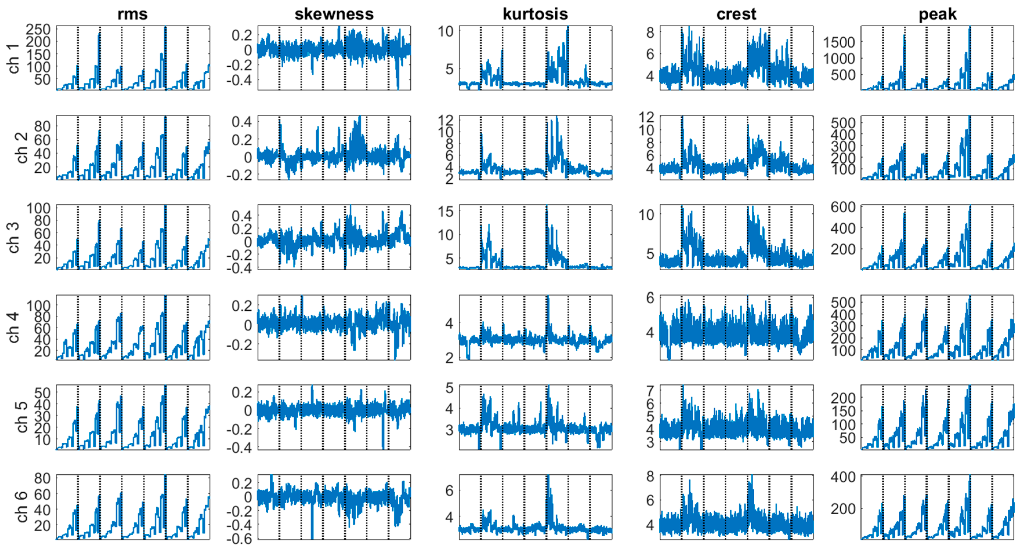
Signal processing: features selection, extraction, and metrics,

(d)

Pattern processing: statistical model development and validation,

(e)

Situation assessment,

(f)

Decision making.

The present work focuses on points (c) and (d), which are in the domain of data mining for damage identification. In this regard, a hierarchical structure defining the steps and the purposes of such damage identification has been previously proposed [2,3]:

• Level 1: Detection—indication of the presence of damage, possibly at a given confidence
• Level 2: Localization—knowledge about the damage location
• Level 3: Classification—knowledge about the damage type
• Level 4: Assessment—damage size
• Level 5: Consequence—actual degree of safety and remaining useful life

The first four are usually included in the definition of diagnostics, while the last one belongs to prognostics. Success at any level obviously depends on having successfully achieved all the prior levels, which are then founded on damage detection, to which this work is devoted.

In particular, hypothesis testing will be used to define a data-based (or driven) damage detection strategy, not relying on a priori knowledge about the system, but on the regularities (i.e., patterns) in the data, which can be considered as the symptoms indicating the possible presence of damage.

1.1. Features

The scope of the present analysis is to link a symptom appearing in the signal to the presence of damage, which corresponds to highlighting patterns in the data. Unfortunately, raw vibration signals are often a disorganized sum of different effects (i.e., arising from several sources) and polluted by noise so that the dominant damage traits are commonly hidden and must be unearthed. Such damage-distinguishing characteristics extracted from the raw signals are commonly called features and their selection is critical as it affects the accuracy and stability of the whole detection process. In particular, a feature is required to be consistent with damage (i.e., it should increase when damage is incremented) and should have high sensitivity in order to reveal incipient damage. Indeed, if a feature shows high fluctuation in the healthy condition, it will be harder to notice a deviation due to damage, unless the damage is severe. Furthermore, the vibration signal is commonly affected by operational (e.g., speed, load) and environmental (e.g., temperature, humidity) variations, which can be seen as latent (i.e., non-measured) confounding factors. A perfect feature to monitor would be to immune these effects and to generate stationary data which is easily processed. Obviously, this idealization is often far from reality and algorithms which compensate for nonstationary confounding influences can be found in the literature (e.g., [4]). Nevertheless, a low sensitivity to such effects is desirable.

To summarize, a good feature should show:

• Damage consistency,
• Damage sensitivity and noise-rejection ability,
• Low sensitivity to unmonitored confounding factors.

In VM, the raw data is commonly a time-series of accelerations measured on the casing of a machine. Most of the vibration is obviously directly linked to the periodic events in the machine’s operation, such as rotating shafts, meshing gear-teeth, etc., so that in the signal spectrum, particular spectral lines (the so-called machine signature) appear. Spectral lines, such as the gear-mesh frequency, are known to be sensitive to damage and are then suitable features. More sophisticated signal processing techniques are currently available (e.g., see [5,6,7,8,9,10]) to highlight the signal of interest with respect to the noise (i.e., to increase the signal-to-noise ratio—to de-noise), to compensate for the transmission path from the source to the sensor and to isolate the different sources to enhance their contribution (e.g., Blind Source Separation). These algorithms can be very effective, but in general, are not ready for working independently from human supervision. Some techniques for damage detection based on lower-level features, on the contrary, can avoid human supervision and outperform the spectral features in terms of repeatability and reliability. In this regard, global statistical features can be found in the literature [11,12]. They are based on the largely proven belief that the presence of a malfunction alters the dynamic response of the system, so that the measured acceleration appears different. Modelling the vibration signal as a random process, excluding at least the presence of confounders, any modification in the probability distribution of the acceleration measurements is ascribable to the presence of a malfunction. Probability is a measure of the likelihood that an event will occur. The discrete variable $y\left(t\right)$, whose discrete realization $y\left(k{T}_s\right)=y\left(k\right)$ is measured at a sampling frequency of $f_s=\frac{1}{T_s}$. This measure can be easily compared to a threshold, $y$. The likelihood of $y\left(k\right)$ being less or equal than the threshold, takes the name of cumulative distribution function (cdf): $P\left(y\right)=prob[y\left(k\right)<y]$. Assuming a continuous cdf, the probability density function (pdf) of such a variable is defined as:

$$p\left(y\right)=\underset{\Delta y\to 0}{lim}\left(\frac{prob\left[y<y\left(k\right)\le y+\Delta y\right]}{\Delta y}\right)=\underset{\Delta y\to 0}{lim}\left(\frac{P\left(y+\Delta y\right)-P\left(y\right)}{\Delta y}\right)=\frac{dP}{dy}$$

(1)

$$\mathrm{with}:p\left(y\right)\ge 0,P\left(y\right)={{\displaystyle \int }}_{-\infty }^{y}p\left(\gamma \right)d\gamma ,{{\displaystyle \int }}_{-\infty }^{+\infty }p\left(y\right)dy=1$$

(2)

In mathematics, in particular in statistics, specific quantitative measures of the shape of a pdf can be computed. These statistical functions summarizing the pdf are called moments, and are defined as:

$${\mu }_n={{\displaystyle \int }}_{-\infty }^{+\infty }{\left(y-c\right)}^{n}p\left(y\right)dy$$

(3)

where $n$ is the moment order, while $c$ is a constant equal to $0$ for the raw moments and corresponding to the mean value for centered moments. When a normalization is performed, the moment is said to be standardized. The most relevant moments are reported in

Table 1. The most widely used moments of a probability distribution function.

Moments	Name	Formulation
Order 1—raw moment: Location	Mean Value	${\mu }_1={\mu }_y=E\left[y\left(k\right)\right]={{\displaystyle \int }}_{-\infty }^{+\infty }yp\left(y\right)dy$
Order 2—central moment: Dispersion	Variance	$\begin{array}{c}{\mu }_2={\sigma }_y^2=E\left[{\left(y\left(k\right)-{\mu }_y\right)}^2\right]\\ ={{\displaystyle \int }}_{-\infty }^{+\infty }{\left(y-{\mu }_y\right)}^{2}p\left(y\right)dy\end{array}$
Order 3—standardized moment: Symmetry	Skewness	$\frac{{\mu }_3}{{\sigma }_y^3}=E\left[{\left(\frac{y\left(k\right)-{\mu }_y}{{\sigma }_y}\right)}^3\right]$
Order 4—standardized moment: “Tailedness”	Kurtosis	$\frac{{\mu }_4}{{\sigma }_y^4}=E\left[{\left(\frac{y\left(k\right)-{\mu }_y}{{\sigma }_y}\right)}^4\right]$

.

For acceleration signals, the mean value is commonly null, so that the distribution results centered in $0$ and the computation of higher order central moments is simplified. In particular, the 2nd order moment corresponds to the square of the so-called Root Mean Square (RMS). In this case, it represents not only the width of the pdf, but also the average power of a stationary process and is a robust measure of the acceleration level. Another level indicator is the peak value, defined as half the difference between the maximum and the minimum acceleration levels. This is commonly much more sensitive to noise. Usually, the ratio of Peak and RMS defines a third level indicator called Crest Factor, which is very reliable in the presence of significant impulsiveness. The level indicators are very commonly used (e.g., in [13]). The most common are summarized in

Table 2. The most widely used level indicators for a discrete signal.

Level Indicators	Name	Formulation
Root Mean Square	RMS	$RMS=\sqrt{E\left[{\left(y\left(k\right)\right)}^2\right]}$
Peak value	Peak	$peak=\frac{\max \left(y\left(k\right)\right)-\min \left(y\left(k\right)\right)}{2}$
Crest factor	Crest	$crest=\frac{peak}{RMS}$

.

The 3rd order moment is a measure of the degree of symmetry around the location, so that symmetric distributions feature skewness $0$, while the value can become either positive or negative if the mean value moves right or left with respect to the peak of the distribution (the mode), respectively.

The 4th order moment is a measure of tailedness that quantifies the importance of the tail extremity and is therefore sensitive to outliers. Due to this, it is sometimes considered the measure of peakedness of the acceleration signal but should not be mistaken for a measure of peakedness of the pdf itself.

In the present work, the most common time-series features here introduced, such as RMS, skewness, kurtosis, peak value and crest factor were selected.

1.2. Pattern Recognition

Once the quantitative features are selected and extracted, an intelligence should be used to univocally relate the statistically significant changes in the features to the presence of damage. This can be performed through a statistical model able to give quantitative information about the estimated state of health and corresponding confidence. This depends on the natural fluctuation of the healthy features, and also on the amount of data used to train the algorithm. Indeed, a statistical model, mimicking the cognitive function of learning (i.e., machine learning), can distinguish the data corresponding to a healthy condition from the data produced by a damaged state. The learning occurs during a training (or calibration) phase which can be supervised or unsupervised. In the first case, the training is completed on labelled data. A training example is a pair of input-output information, as the corresponding state of health is known. On the contrary, in the case of unsupervised learning, no label is available. The unsupervised problem generally takes the name of clustering, while the supervised is called classification.

In the field of damage identification, the Level 1 problem of damage detection appears to involve two groups alone—healthy and damaged. Furthermore, in many cases, acquisitions from a damaged condition are not possible because of safety issues, so that earning should rely only on healthy acquisitions with a semi-supervised learning. In this case, the binary classification problem can be tackled via novelty detection.

1.3. Methodology

This work is devoted to the exploration of hypothesis testing as a tool for analysing the value-type data extracted from a signal (i.e., the features) and recognizing the patterns which characterize a damaged condition. The subject of hypothesis testing is introduced from the beginning and applied to the framework of damage detection. The considerations which hold for the univariate case are then extended to multivariate datasets in which multiple features extracted from multiple acceleration measurements are treated together. In VM, it is common to introduce redundancy in the data by using more than one sensor, so that a preliminary consistency check can highlight possible failures in the sensing devices. This introduces a form of self-monitoring of the diagnostic system itself, which becomes more reliable and robust.

The use of multivariate analysis accounting for the correlation structure of a dataset is a very effective way for fusing the information contained in the different features. The dataset is then compressed, identifying and eliminating only statistical redundancy, while the effect of damage is enhanced at the same time. A simple way for performing this kind of data fusion is a dimensionality reduction to a 1-D variable that summarizes the entire dataset.

In the literature, the simplest algorithm, typically used for visualization purposes, is the principal component analysis (PCA) [14]. In short, PCA finds a transform (i.e., a rotation) of the original reference frame matching the directions which explain most of the data variability (i.e., the variance). By selecting the first two or three components, and projecting (or mapping) the multivariate dataset into these reduced spaces, 2-D or 3-D representations can be found. If just the first component is left, a linear combination of the features which summarizes the entire dataset is found.

In this direction, variability is maximum, but this does not always imply that the two classes of interest are optimally separated. Nevertheless, a projection maximizing a measure of distance of the two distributions (i.e., the effect size) can be found through Fisher’s linear discriminant analysis (LDA) [15].

In any case, the PCA dimensionality reduction can be regarded as a lossy compression, as some portion of the original multivariate dataset variability is neglected. In general, nothing ensures that the damage information is contained in the first principal component. On the contrary, in many cases, the first components prove to represent strong latent effects such as operational (e.g., speed, load) and environmental (e.g., temperature, humidity) variations.

A lossless non-linear 1-D dimensionality reduction can be found through novelty detection via Mahalanobis distance [16]. In this regard, the information about novelty (i.e., deviation from normality) is additive in the space dimensions, so that the whole variability is preserved. Furthermore, it automatically accounts for compensation of linear or quasi-linear hidden confounding effects by weighting the distance on the different principal components, so that information about the direction is included, differently from LDA.

In this analysis, these three methods are compared on the open-access dataset using high-speed aeronautical rolling bearings described in [12], from a test rig developed by the Dynamic and Identification Research Group (DIRG) of the Department of Mechanical and Aerospace Engineering at Politecnico di Torino.

To conclude, the problems related to high dimensionality (i.e., the curse of dimensionality) and to the selection of the sample size n were examined.

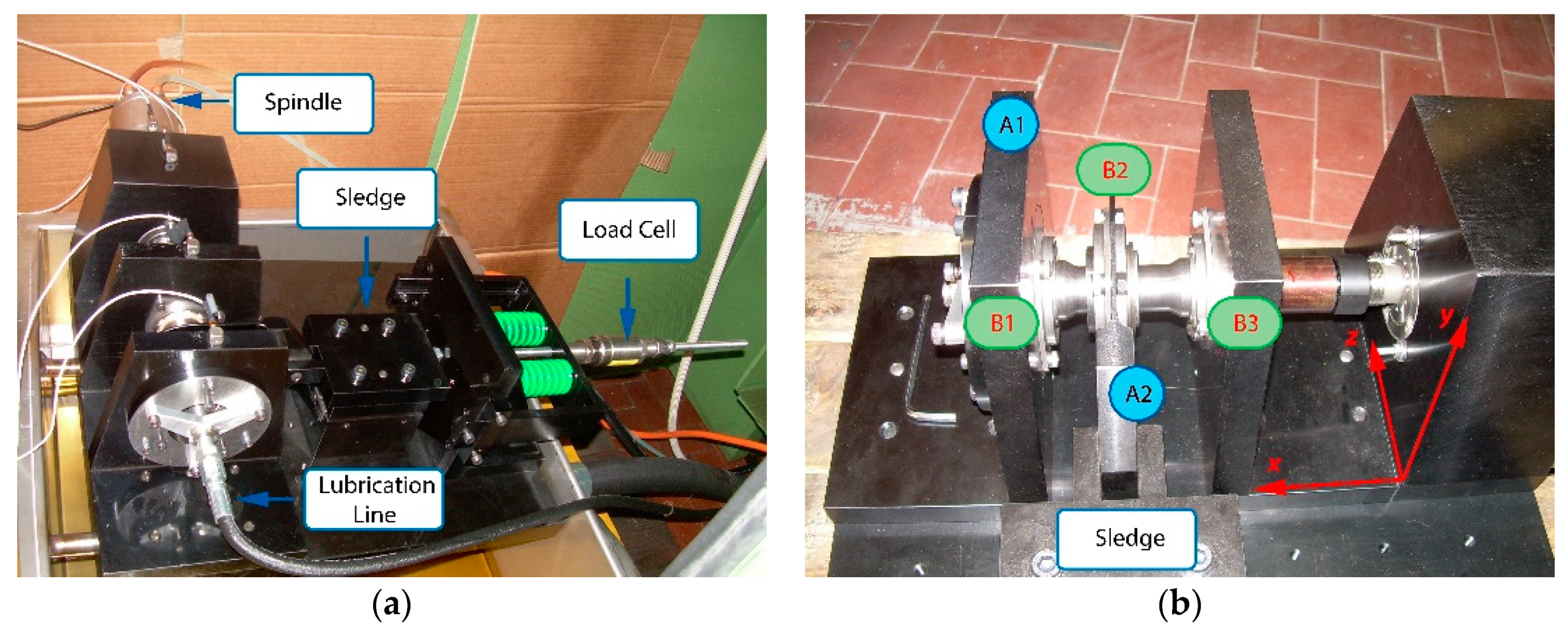
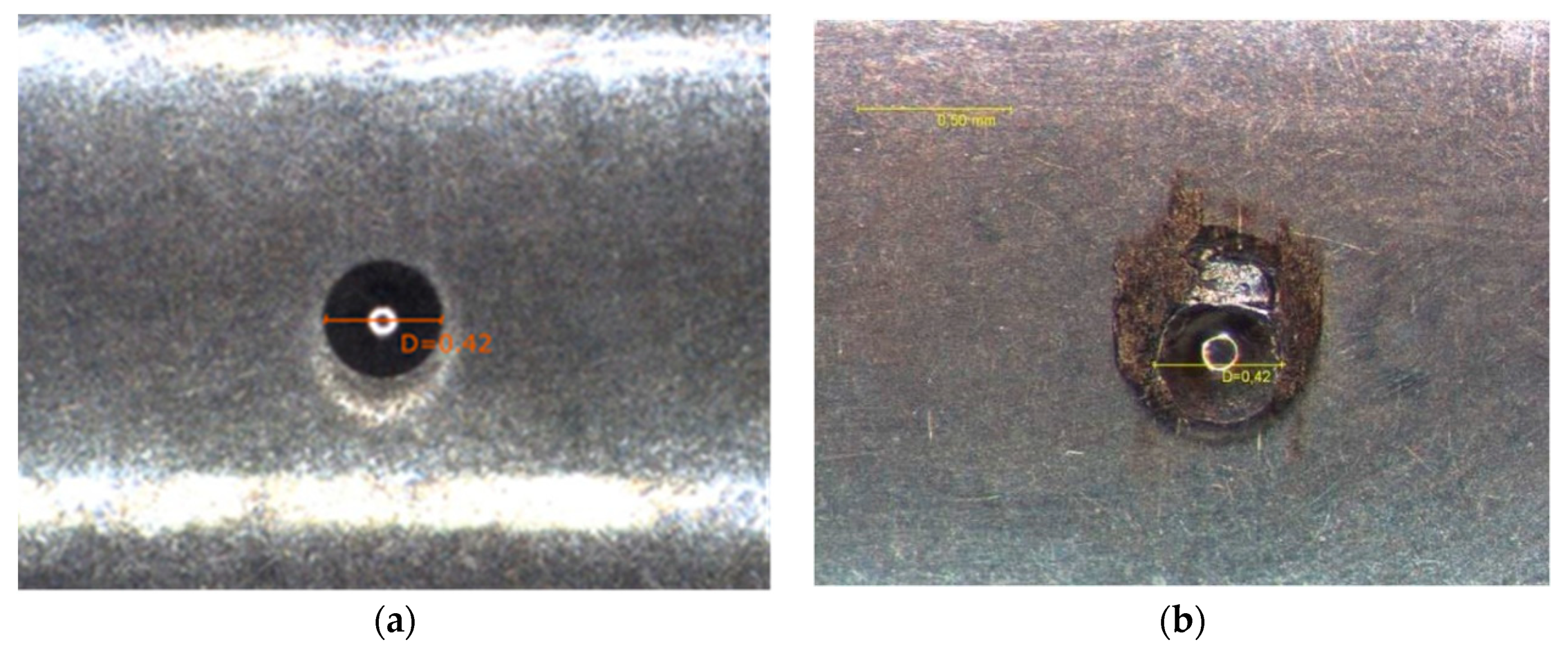
1.4. The Experimental Setup and the Dataset

The considered test rig consists of a direct drive rotating shaft supported by two identical high-speed aeronautical roller bearings (B1 and B3 in Figure 1), one of which (the farthest from the motor, identified as B1) exhibits the different health conditions reported in

Table 3. Bearing B1 codification according to damage type (inner ring or rolling element) and size. The damage is obtained through a Rockwell tool producing a conical indentation of maximum diameter reported as characteristic size.

Code	0A	1A	2A	3A	4A	5A	6A
Damage type	none	Inner Ring	Inner Ring	Inner Ring	Rolling Element	Rolling Element	Rolling Element
Damage size [µm]	-	450	250	150	450	250	150

. A third central bearing (B2) was used to load the shaft with an increasing force of 0, 1000, 1400 and 1800 N, while the speed was set at four different values of approximately 90, 180, 280, 370, 470 Hz for a total number of 17 combinations of load and speed (see

Table 4. The operational conditions: Speed and load combination.

Label	1	2	3	4	5	6	7	8	9	10	11	12	13	14	15	16	17
$f$ [dHz]	9	9	9	9	18	18	18	18	28	28	28	28	37	37	37	47	47
$F$ [kN]	0	1	1.4	1.8	0	1	1.4	1.8	0	1	1.4	1.8	0	1	1.4	0	1

). The structure is equipped with two tri-axial accelerometers positioned on the bearing supports B1 (accelerometer A1, as reported in Figure 1) and on the loading sledge bearing B2 (accelerometer A2), sampled at a frequency fs of 51,200 Hz for a duration of T is 10 s.

In order to explore the available data, the features introduced in Section 1.1 were computed on shorter independent chunks (i.e., no overlap) of the original available data to ensure statistical reliability. The number of subdivisions was chosen with particular care, to balance the significance both on the features extraction, and on the further analysis. According to considerations in Section 2.4.2, each of the 17 acquisitions (see Table 4) was subdivided in one hundred 0.1 s parts, on which the 5 features were extracted.

Finally, per each health condition, 1700 observations in a 30-dimensional space (6 channels, 5 features) were obtained. The health condition ranges from healthy (0A) to the different damages on inner ring and rolling element reported in Table 3. The dataset is finally summarized in Figure 2 and Figure 3.

The raw data are further described in [12] and can be downloaded at ftp://ftp.polito.it/people/DIRG_BearingData/.

2. The Methods

In this section, the proposed methods are described in detail, starting from the fundamentals of statistics and hypothesis testing.

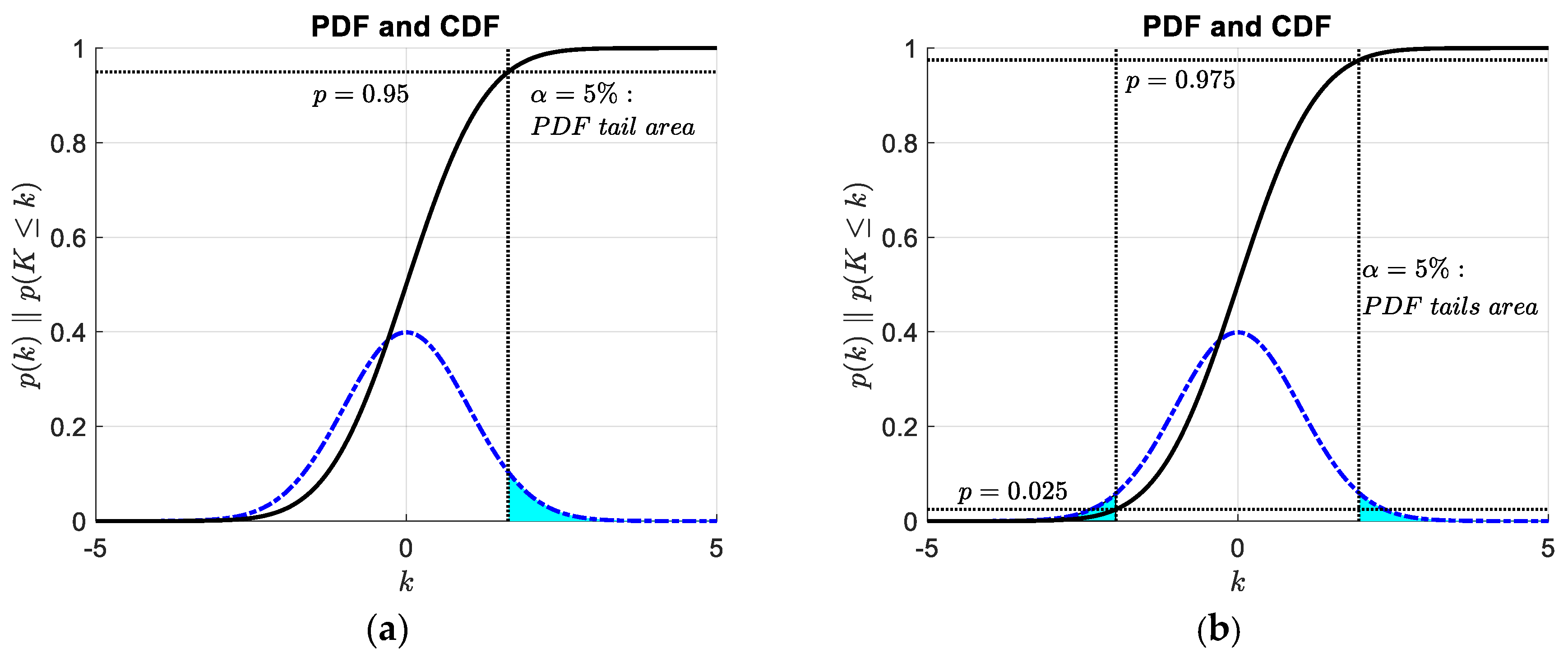
2.1. Statistics and Probability: An Introduction to Hypothesis Testing

Statistics is a branch of mathematics dealing with data collection, organization, analysis, interpretation and presentation. The word is first introduced in the English vocabulary by Sir John Sinclair in 1829 with the meaning, numerical data collected and classified. It comes from the German Statistik introduced by Gottfried Achenwall (1749) to originally designate the analysis of data about the state (from the Italian “statista”, meaning statesman, politician and descending from the Latin word “status” meaning position, place, condition, or figuratively, public order).

In particular, the word, statistics, can be interpreted as the investigation of large numbers or theory of frequencies [17]. According to the von Mises definition of the term, statistics is then linked to probability theory. Indeed, despite being in common language, the word, probability, refers to the measure of the likelihood that an event will occur (from 0 i.e., impossible to 1 i.e., certain). The frequentist definition is much stricter:

The probability is the limiting value of the relative frequency of a given attribute within a considered collective. The probabilities of all the attributes within the collective form its distribution.

The starting point of the probability theory is the concept of a collective (or population), an infinite sequence of observations, each consisting in the recording of a certain attribute. The fundamental frequentist axiom follows. Selecting just $n$ recordings (a new finite collective is formed by the selection of a sample from the population), the relative frequency of an attribute, $n_1/n$, approaches a constant limiting value when $n$ is increasing indefinitely. From this axiom, the law of large numbers (LLN) can be derived. Actually, the LLN can be also approached via alternative points of view, such as the Bernoulli-Poisson or the Bayes’s. In any case, the LLN states that the sample average $\overline{x_n}=\frac{1}{n}{\displaystyle \sum }{x}_i$ converges to a constant limiting value, i.e., the true expected value $\mu$, for an increasing $n\to \infty$. This can be further generalized to any statistical function (e.g., the median, the variance, etc.), namely a function depending on the true frequency distribution, but not on the order of the observations or their total number.

By focusing on the LLN applied to the mean, it is easy to get a proof involving the known, true statistical functions $E\left[x_i\right]=\mu$, $var\left[x_i\right]={\sigma }^2$ and the simple definitions of expectation and variance:

$$E\left[\overline{x_n}\right]=\frac{1}{n}E\left[{\displaystyle \sum }{x}_i\right]=\frac{1}{n}{\displaystyle \sum }E\left[x_i\right]=\frac{n\mu }{n}=\mu$$

(4)

$$var\left[\overline{x_n}\right]=\frac{1}{n^2}var\left[{\displaystyle \sum }{x}_i\right]=\frac{1}{n^2}{\displaystyle \sum }var\left[x_i\right]=\frac{n{\sigma }^2}{n^2}=\frac{{\sigma }^2}{n}$$

(5)

Therefore, $n\to \infty$, $var\left[\overline{x_n}\right]\to 0$, implying $\overline{x_n}\to \mu$.

Furthermore, it can be proved that, for any generic sample distribution featuring finite statistical functions $E\left[x_i\right]=\mu$ and $var\left[x_i\right]={\sigma }^2$, as $n$ approaches infinity, the variable $\overline{x_n}$ asymptotically converges in distribution to a normal distribution $N_{\left(\mu ,\frac{{\sigma }^2}{n}\right)}$. This corresponds to the so-called central limit theorem (CLT), the name given in 1920 by the mathematician, Polya, to the Gauss’s theory of errors derived by Laplace’s exponential law. That is, the overall error induced by the sum of many small elementary errors follows an exponential distribution, which takes the name of the Gaussian bell curve.

Due to the nature of frequentist probability as a limiting value for $n\to \infty$, in practical cases, the true probability distribution and related statistical functions are never known a-priori but can be inferred from a sample i.e., extrapolated from the sample to the population. For example, the mean value, $\overline{x_n}$ can be used as an estimator of $\mu =\overline{x_{\infty }}$ at a given confidence or significance (i.e., the result is convincing up to some degree of trust).

Consider the CLT. Taking $\overline{x_n}$ as estimator, the dispersion of its normally distributed values is given by $var\left[\overline{x_n}\right]=\frac{{\sigma }^2}{n}$. Then, the true expected value $\mu$ falls in an interval $\left(\overline{x_n}-\frac{\sigma }{\sqrt{n}},\overline{x_n}+\frac{\sigma }{\sqrt{n}}\right)$ at a confidence $1-\alpha =68\%$ (or significance $\alpha =32\%$). Standardizing the estimator as $z_n=\frac{\overline{x_n}-\mu }{\sigma /\sqrt{n}}$, it is possible to derive the results in

Table 5. Common Confidence Intervals for a Gaussian variable [18].

Standard Interval	Inside to Outside Ratio	$\mathbf{Confidence}1-\mathit{\alpha }$
$\pm 0.6745$	$1\mathrm{to}1$	$50\%$
$\pm 1$	$2.15\mathrm{to}1$	$68.3\%$
$\pm 2$	$21\mathrm{to}1$	$95.5\%$
$\pm 3$	$369\mathrm{to}1$	$99.7\%$

, which holds for any Gaussian distribution.

Generalizing, a critical value for the given confidence can be always found to form a confidence interval such that:

$$-N_{\left(0,1\right),\frac{\alpha }{2}}\le z_n\le N_{\left(0,1\right),\frac{\alpha }{2}}$$

(6)

$$\overline{x_n}-\frac{\sigma }{\sqrt{n}}{N}_{\left(0,1\right),\frac{\alpha }{2}}\le \mu \le \overline{x_n}+\frac{\sigma }{\sqrt{n}}{N}_{\left(0,1\right),\frac{\alpha }{2}}$$

(7)

Some definitions are needed. A confidence interval (CI) is a type of interval estimate giving a range of values in which the true, unknown population parameter falls at chosen probability rate (i.e., the confidence, $1-\alpha$). The critical value which limits the interval is the value exceeded only $100\frac{\alpha }{2}$ times in a hundred, and is given by $N_{\left(0,1\right),\frac{\alpha }{2}}$.

Unfortunately, the population variance ${\sigma }^2$ in most of cases is unknown. When $n$ is large, the variance can be estimated from the sample, as well as for the mean.

The maximum-likelihood (ML) estimate of the sample variance is given by $s_{n,ML}^2=\frac{1}{n}{\displaystyle \sum }{\left(x_i-\overline{x_n}\right)}^2$, while the unbiased estimator can be found as $s_n^2=\frac{1}{n-1}{\displaystyle \sum }{\left(x_i-\overline{x_n}\right)}^2$.

If the sample variance is used in place of the true variance, the formula given for the confidence interval of the mean (Equation (7)) holds for large $n$, so that:

$$\overline{x_n}-\frac{s_n}{\sqrt{n}}{N}_{\left(0,1\right),\frac{\alpha }{2}}\le \mu \le \overline{x_n}+\frac{s_n}{\sqrt{n}}{N}_{\left(0,1\right),\frac{\alpha }{2}}$$

(8)

Otherwise, if the sample size is small (typically $n<30$), it can be proved that a standardization leads to:

$$t_n=\frac{\overline{x_n}-\mu }{s_n/\sqrt{n}}~t_{\left(n-1\right)}$$

(9)

where $t_{n-1}$ is a student’s t distribution with $n-1$ degrees of freedom. Hence, a correction of the confidence interval for the mean follows:

$$\overline{x_n}-\frac{s_n}{\sqrt{n}}{t}_{\left(n-1\right),\frac{\alpha }{2}}\le \mu \le \overline{x_n}+\frac{s_n}{\sqrt{n}}{t}_{\left(n-1\right),\frac{\alpha }{2}}$$

(10)

It is noted for $n\to \infty$, $t_{\left(n-1\right),\alpha }\to N_{\left(0,1\right),\alpha }$ and $s_n\to \sigma$, so that this CI tends to be the one given in Equation (7) when $n$ increases.

This demonstrates how inferential statistics can extrapolate information from the sample to the population at a confidence depending on the size of the sample. The estimation theory is not the only subject of inferential statistics. Hypothesis testing is also fundamental [19,20].

A statistical hypothesis test is a method of statistical inference that is meant to compare two statistical samples, or a sample against a model. A hypothesis is proposed for the statistical relationship among the two and this is compared to an alternative suggesting no relationship. The comparison is deemed statistically significant if the relationship can be proved to be an unlikely realization of the null hypothesis according to a threshold probability (i.e., the confidence). This is strictly related to the idea of a confidence interval.

As hypothesis testing can be tackled through confidence intervals via the computation of critical values, it is far more common to compute the so-called p-value. The p-value (i.e., probability value or asymptotic significance) is the probability that, given $H_0$, the statistical summary is more extreme than the actual observed results. Hence, if this p-value is less than or equal to a selected significance level $\alpha$, the hypothesis is rejected in favour of the $H_a$. Depending on the point of view, the phrase, more extreme than, can take different meanings, as summarized in

Table 6. Hypothesis testing: p-value logic.

Tails	Confidence Interval
For a right tail event, it can be stated as	$\mathrm{Pr}(K\ge k|H_0)$
For a left tail event, it is	$\mathrm{Pr}(K\le k|H_0)$
For a double tail event (on a symmetric distribution), it becomes	$2\min \left(\mathrm{Pr}\left(K\ge k|H_0\right),\mathrm{Pr}(K\le k|H_0)\right)$

. The graphical interpretation is given in Figure 4.

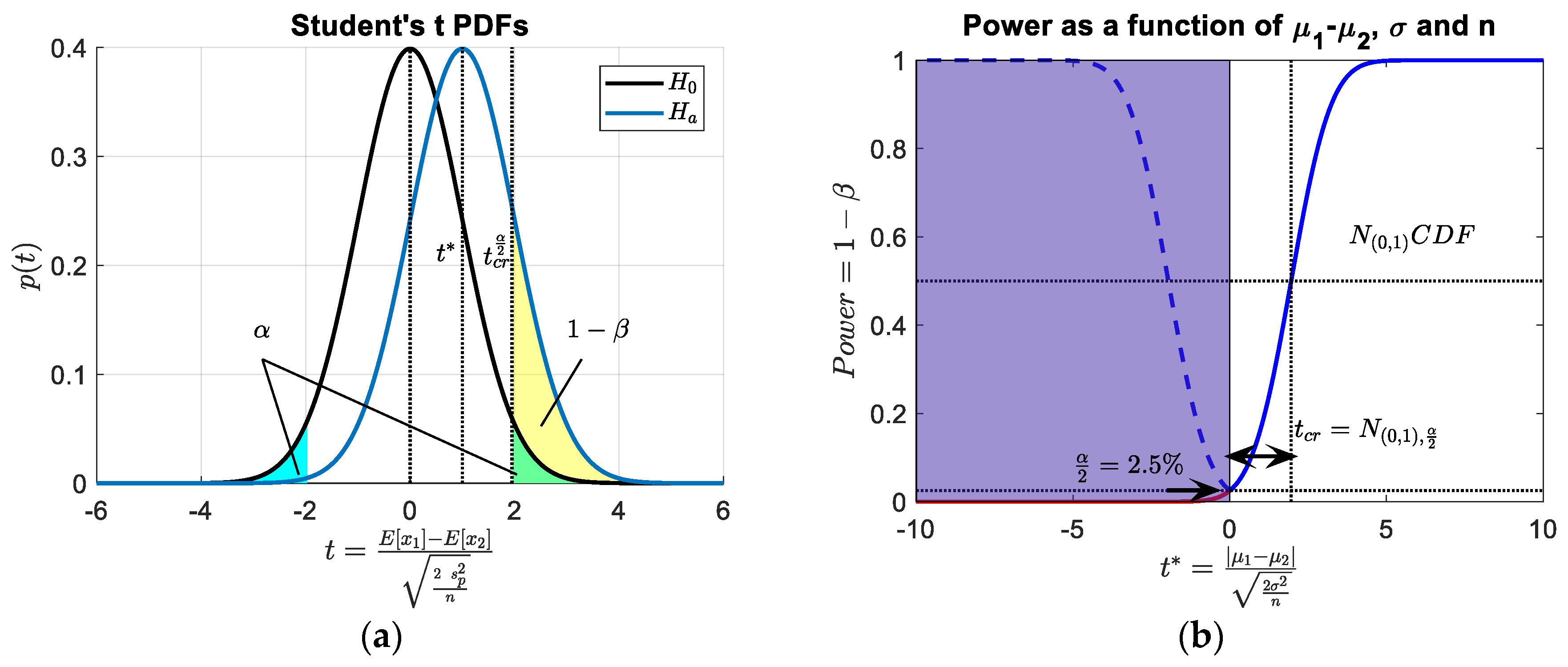
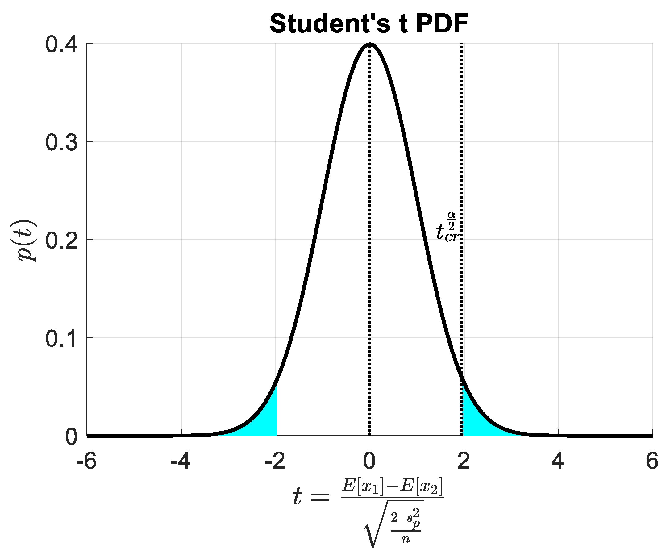
2.1.1. Hypothesis Testing of the Difference between Two Population Means

A two-sample location test of the null hypothesis, $H_0:{\mu }_1={\mu }_2$, namely that the two population means are equal, can be performed against the alternative hypothesis $H_a:{\mu }_1\ne {\mu }_2$. When it can be assumed that the two distributions have the same variance (i.e., homoscedasticity) and the samples come from the distributions in

Table 7. Statistical summary of the sample as a function of the population distribution and numerousness $n$ of the sample.

Distribution of the Population:	Statistical Summary of the Sample:
Normal distributions with given variance or Generic distributions (also non-normal) assuming $n>30$, thanks to CLT	$z=\frac{E\left[x_1\right]-E\left[x_2\right]}{\sqrt{{\sigma }_1^2/n_1+{\sigma }_2^2/n_2}}~N_{\left(0,1\right)}$
Normal distributions with unknown variance	$t=\frac{E\left[x_1\left]-E\right[x_2\right]}{\sqrt{s_p^2/n_1+s_p^2/n_2}}~t_{\left(n_1+n_2-2\right)}$

, the corresponding statistical summary and its distribution are well defined. Therefore, it is easy to create a test for the null hypothesis, as graphically shown in Figure 5. The formulas in Table 7 are based on the pooled estimate $s_p$ of the unknown variance of the two samples ($i=1,2$):

$$\begin{array}{c}\mathrm{Biased}\mathrm{estimate}:s_{p,B}^2=\frac{{{\displaystyle \sum }}_i\left(n_i-1\right)s_i^2}{{{\displaystyle \sum }}_i{n}_i}\\ \mathrm{Unbiased}\mathrm{estimate}:s_p^2=\frac{{{\displaystyle \sum }}_i\left(n_i-1\right)s_i^2}{{{\displaystyle \sum }}_i\left(n_i-1\right)}\end{array}$$

(11)

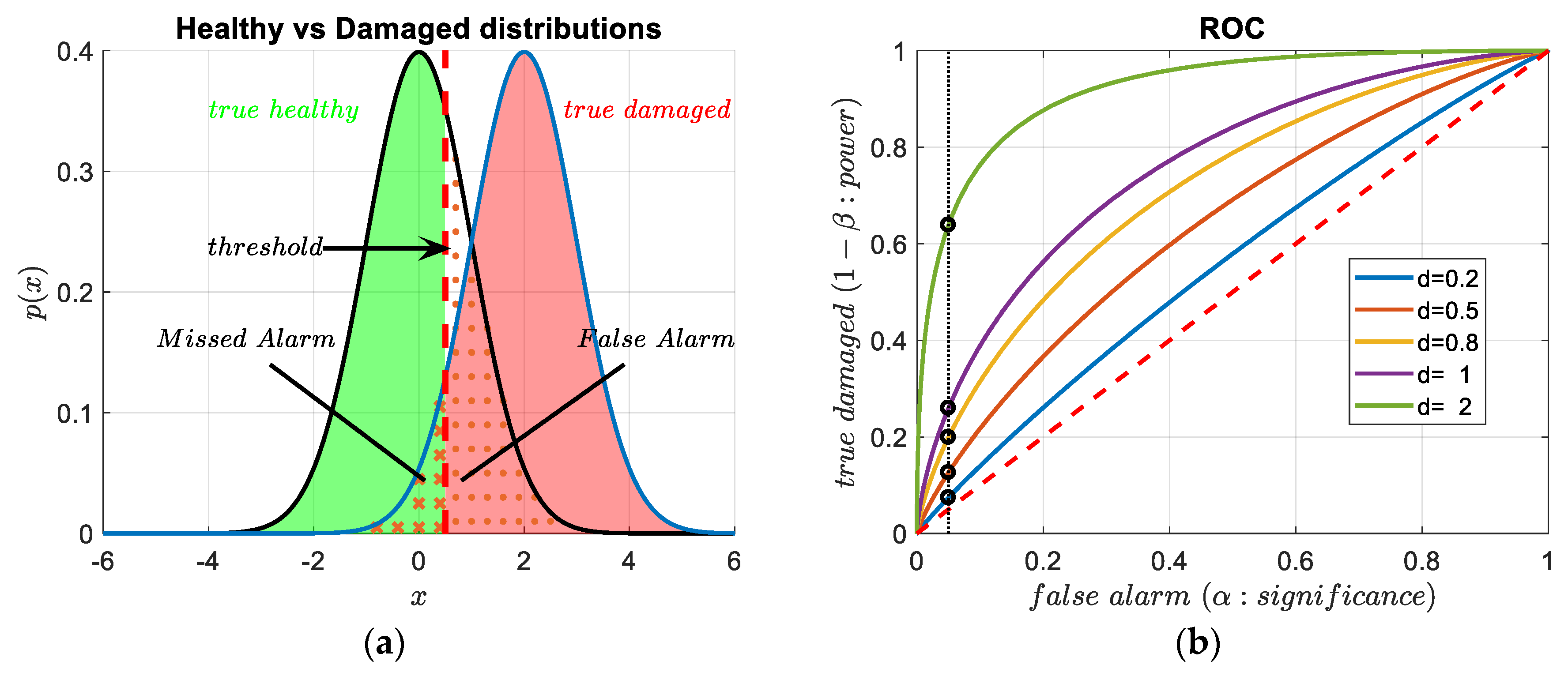
2.1.2. Diagnostics, Hypothesis Testing and Errors

Adopting the null hypothesis, $H_0:\mathrm{the}\mathrm{machine}\mathrm{is}\mathrm{healthy},$ a new sample from the machine under investigation can be compared to a reference healthy sample acquired in a calibration stage (known as healthy), implying then: $H_0:{\mu }_{new}={\mu }_{ref}$. This is obviously linked to statistical classification and is therefore fundamental to perform Level 1 diagnostics.

Classification refers to the problem of identifying which category (in the considered case, just two options, healthy versus non-healthy) a new observation (i.e., a point in the feature space) belongs, based on a training data set taken as reference. This set is labelled, as the data points are known (or at least believed at a high confidence) to come from a given health condition. Classification is always a two-step procedure:

(a)

In the training phase, the labelled samples are used to build a classifier, namely a function which divides the feature (variable) space into groups. This separation is then found in terms of distributions. When a single feature is used to investigate the machine, the classifier function corresponds to the selection of a threshold. It is relevant to point out that this feature-space partitioning can also be obtained in an unsupervised way (i.e., without exploiting the labels). This takes the name of clustering.

(b)

In a second phase, the new observations are assigned to the corresponding class (i.e., classified) according the classifier function. Each new unlabelled data point is then treated individually.

Typically, a validation phase is added between these two steps to assess the performances of the classifier function, out of sample, namely on data points different from the ones used for the training.

According to these considerations, hypothesis testing is closely linked to classification. Nevertheless, classification implies the knowledge (or at least the belief) that the different samples are not coming from the same distribution, so that the alternative hypothesis takes much more relevance.

Furthermore, an additional step is needed to fully understand hypothesis testing. Imagine the case in which a difference among the means is present (i.e., $H_a$ is true). If $H_0$ is rejected, it means that the two population averages are discriminable. Obviously, if the difference is small, a huge sample size $n$ is needed to detect the difference at significance $\alpha$. In fact, for an increasing $n$, the resolution of the test (i.e., the minimum significant distance between two means according to which $H_0$ is rejected) can be reduced at will.

As $H_a$ is true, then ${\mu }_1-{\mu }_2=D^{*}\ne 0$ and two options are possible:

$$\begin{array}{l}{H}_{0}accepted:\left|\frac{E\left[x_1\right]-E\left[x_2\right]}{\sqrt{2s_p^2/n}}\right|=\left|t{|}_{H_a}\right|\le t_{cr}^{\frac{\alpha }{2}};\mathrm{Probability}:\beta \\ H_{0}rejected:\left|\frac{E\left[x_1\right]-E\left[x_2\right]}{\sqrt{2s_p^2/n}}\right|=\left|t{|}_{H_a}\right|>t_{cr}^{\frac{\alpha }{2}};\mathrm{Probability}:1-\beta \end{array}$$

(12)

Focusing on the true distribution of $t{|}_{H_a}$, this will be centred on $t{}^{*}=\frac{{\mu }_1-{\mu }_2}{\sqrt{2{\sigma }^2/n}}$. Starting from this definition, it is easy to get the value of $d{}^{*}=\frac{{\mu }_1-{\mu }_2}{\sigma }=\frac{D{}^{*}}{\sigma }=t^{*}\sqrt{2/n}$, the so-called effect size, while the probability of rejection $1-\beta$ is commonly identified as the power of the test.

In any case, the test does not consider whether $D_{cr}^{\frac{\alpha }{2},n,\sigma }=\sigma \sqrt{2/n}{t}_{cr}^{\frac{\alpha }{2}}$, namely the minimum resolved distance, is physically meaningful or not, as this consideration also depends on the original populations’ variance, $\sigma ,$ and on the numerousness of the sample size, $n$. Furthermore, no information about the probability of resolving a given $d^{*}$ (i.e., the power) is taken into account by the test itself. These considerations should come prior to the test, at a design of experiment (DOE) stage.

The power of a two population means test is visualized in Figure 6a for a particular $t^{*}$, and generalized for any $t^{*}$ in Figure 6b. This second curve was obtained by shifting the cumulative distribution function (cdf) of the $t_{\left(2n-2\right)}$. For $n>30,$ the student’s t distribution is practically equal to a standard normal, whose cdf is used in this case to obtain the graph of Figure 6b (which holds even for smaller $n$ if a known variance $\sigma$ is substituted to the estimated $s_p$).

As $\alpha =5\%$ is probably the most common value and is rarely changed, this graph can be used at a DOE stage to evaluate the optimal $n$ able to resolve an expected effect size at a probability $1-\beta$ larger than a selected value. This $d^{*}$ can be approximated from prior research as ${\widehat{d}}^{*}=\left|\frac{E\left[x_{dam}\left]-E\right[x_{ref}\right]}{s_p}\right|$, or through conventions, such as the one proposed by Cohen [20] and here reported in

Table 8. General rule for a rough quantification of the effect size [20].

Effect Size	${\mathit{d}}^{*}$
Small	$0.2$
Medium	$0.5$
Large	$0.8$

.

For example, for having a power $1-\beta =0.8$, the graph in Figure 6b gives $t^{*}=\left|\frac{{\mu }_1-{\mu }_2}{\sqrt{2{\sigma }^2/n}}\right|=2.8$ which implies, at least, $n=2{\left(\frac{2.8}{d^{*}}\right)}^2$. Therefore, for detecting a large effect size, the so-computed $n\cong 25$ is enough, but the required $n$ increases to $63$ for a medium and to $392$ for a small effect size. As $n$ is obviously limited by physical constraints, a trade-off between confidence $1-\alpha$ and power $1-\beta$ is always necessary to control both the $\mathrm{type}\mathrm{I}$ and $\mathrm{II}$ error rates.

From a diagnostics point of view, the confidence $1-\alpha$ associated to the test implies a $\mathrm{type}\mathrm{I}\mathrm{error}\mathrm{rate}$ (i.e., the significance $\alpha$) which corresponds to the probability of rejecting a true $H_0.$ This must be as small as possible, as a too high a number of triggered false alarms (FA) can erode the confidence of the damage detection. At the same time, the $\mathrm{type}\mathrm{II}\mathrm{error}\mathrm{rate}$ should be kept under control. This is the probability of failing to reject a false $H_0$, usually referred to as $\beta$, the complementary of the power of the test. This value corresponds to a missed indication of damage which is present (missed alarm, MA) and is very detrimental, as it can bring serious economic and life-safety implications. These error rates are usually collected in tables such as

Table 9. Type I and II errors in hypothesis testing for condition-based maintenance (CBM).

		True Health Condition:
		Healthy (H0)	Damaged
CBM Actions	accept ${\mathrm{H}}_0$: Healthy	No Alarm— true healthy	Missed Alarm— type II error
	reject ${\mathrm{H}}_0$: Damaged	False Alarm— type I error	Alarm— true damaged

, which are very common when binary classification is considered. If classification involves more than two groups, larger tables can be found with the name of confusion matrices.

On the contrary, in the field of operational research (OR), a discipline that deals with the application of analytical methods for making better decisions, the receiver operating characteristic (ROC) is usually preferred for assessing the diagnostic ability of a binary classifier while its discrimination threshold is varied.

The interpretation of the critical value as a threshold allows the understanding of how this can be varied to find the best compromise between $\alpha$ and $\beta ,$ and to assess the overall performance of the test or of the classification. Figure 7b summarizes true damaged rate (the power $1-\beta$) as a function of false alarm rate (the significance $\alpha$) for some relevant effect sizes, while the threshold takes all the possible values. The threshold corresponding to the $\alpha =5\%$ critical value is highlighted. In general, the farthest away the ROC curve is from the 1st–3rd quadrant bisector, the better the classification, which improves as the effect size is enlarged.

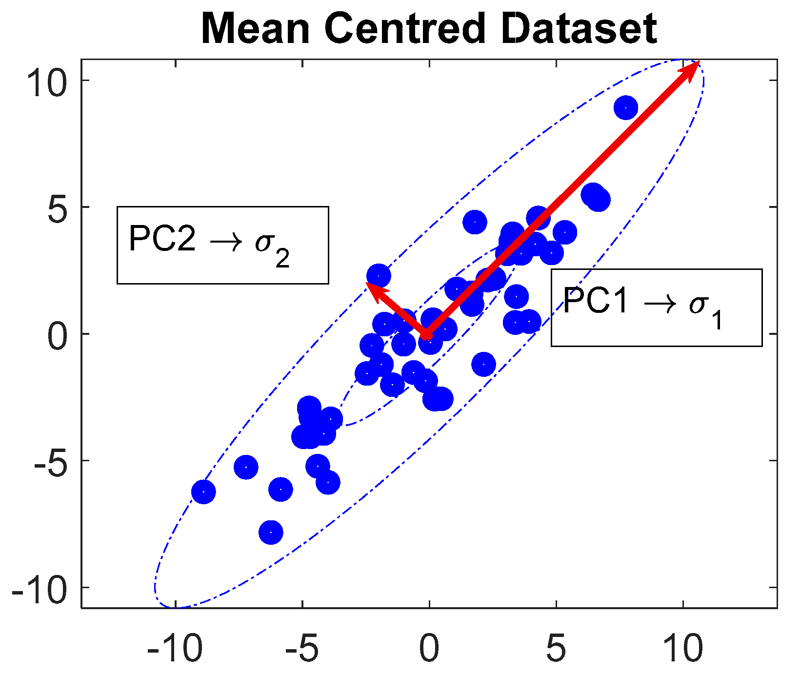
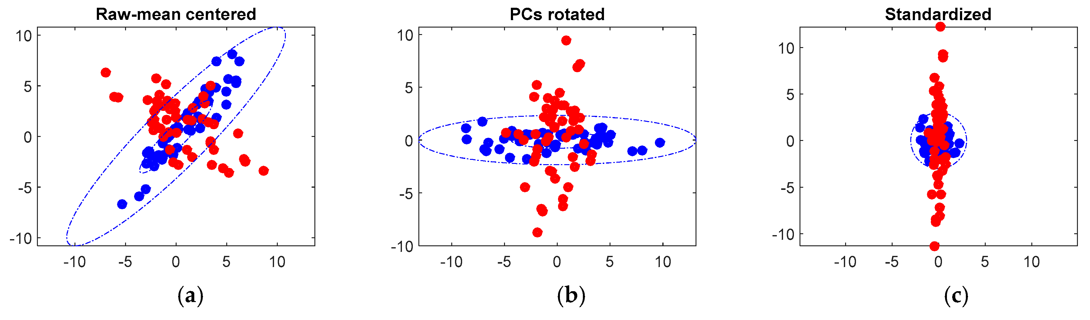
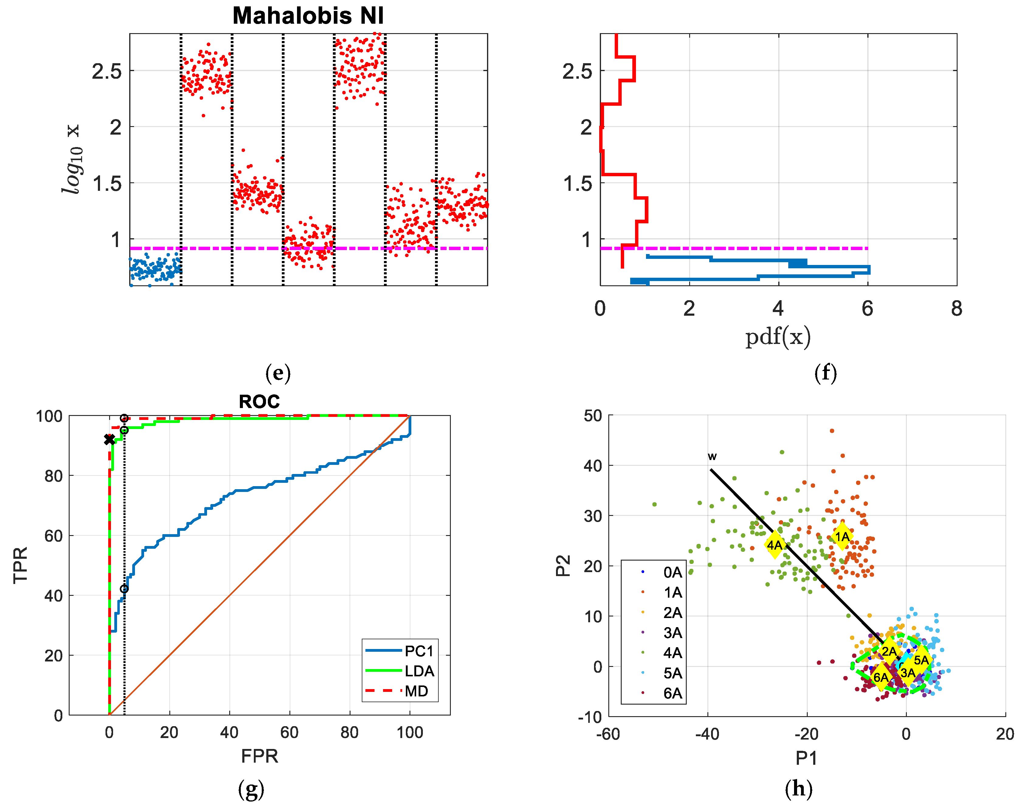
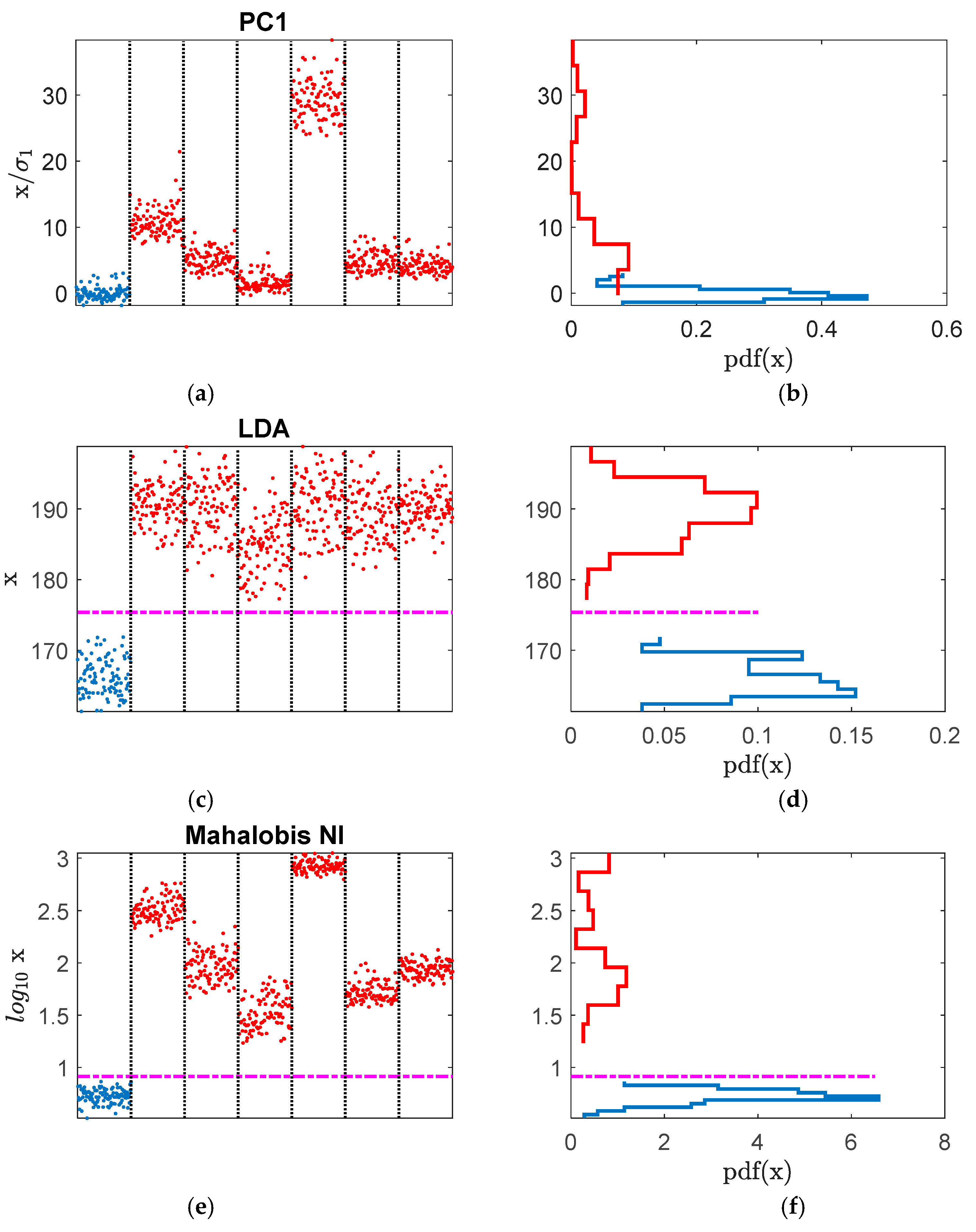
2.2. Principal Component Analysis (PCA)

PCA is a technique which uses an orthogonal space transform to convert a set of correlated quantities into uncorrelated variables called principal components [14,21]. This transformation is basically a rotation of the feature space in such a way that the first principal component will explain the largest possible variance, while each succeeding component will show the highest possible variance under the constraint of orthogonality with the preceding ones. This is usually accomplished by eigenvalue decomposition of the data covariance matrix or singular value decomposition of the data matrix after mean centring.

In general, the main application of PCA is for reducing a complex data set to a lower dimension using the first few components that explain the majority of the variation. This dimensionality reduction is commonly used to obtain 2D or 3D projections of multivariate datasets which are easily visualizable. Furthermore, this can eventually reveal hidden dynamics.

Mathematically, given a $d$-dimensional centred dataset of $n$ observations $X\in R^{d\times n}$, an unbiased estimator for the covariance can be used to obtain:

$$S=\frac{1}{n-1}XX\prime$$

(13)

PCA corresponds to the solution of the eigenproblem:

$$SV=V\mathsf{\Lambda }$$

(14)

where $V$ is the orthogonal matrix ($V^{t}V=V{V}^t=I\to V^{-1}=V^t$) whose columns are the $d$ eigenvectors $v_j$ while $\mathsf{\Lambda }$ is the diagonal matrix of the $d$ eigenvalues ${\lambda }_j$ (usually sorted in descending magnitude) of the matrix $S$.

The matrix $V$ can be used then to decorrelate the dataset $X$, that is, to rotate the reference frame to the one identified by the eigenvectors (i.e., the principal components, PCs) of matrix $S$:

$$Z=V\prime X$$

(15)

If the eigenvectors in $V$ are normalized to have unit length ($v_j^{\prime }{v}_j=1$), the transform is a pure rotation, and it can be proved that ${\sigma }_j^2=var\left(z_j\right)={\lambda }_j$. Namely, the diagonal $\mathsf{\Lambda }$ is the covariance matrix of $Z$. Different normalizations are obviously possible, even if less common.

The geometric interpretation of PCA is related to the fact that an ellipsoid centred in the origin can be associated to any positive definite matrix such as the covariance $S$. Its equation is $X^{\prime }{S}^{-1}X=1$. Therefore, the eigenvectors of $S^{-1}$ define the principal axes of the ellipsoid while the eigenvalues of $S^{-1}$ are the reciprocals of the squares of the semi-axes. This can be verified remembering that the eigenvectors of $S^{-1}$ are the same as the eigenvectors of $S$ and the eigenvalues of $S^{-1}$ are the reciprocal of those of $S$. Indeed, using the inverse transformation $X=VZ$:

$$X^{\prime }{S}^{-1}X=Z^{\prime }{V}^{\prime }{S}^{-1}VZ=Z^{\prime }{\mathsf{\Lambda }}^{-1}Z={{\displaystyle \sum }}_j\frac{z_j^2}{{\lambda }_j}=1$$

(16)

which is the equation of an ellipsoid whose half principal axes are $\sqrt{{\lambda }_j}={\sigma }_j$ long. To visualize the whole geometrical interpretation, Figure 8 is added.

After these considerations, a dimensionality reduction is easily obtained considering the projection of the original $X$ on the first PC explaining most of the dataset variability.

$$z_1=v_1^{\prime }X=v_{11}{x}_1+v_{12}{x}_2+\cdots +v_{1d}{x}_d={\displaystyle \sum }_{k=1}^d{v}_{1k}{x}_k$$

(17)

Equation (17) is basically a linear combination of the $d$ features according to the weights given by the first eigenvector and shows the greatest variance ${\sigma }_1^2=var\left(z_1\right)={\lambda }_1$.

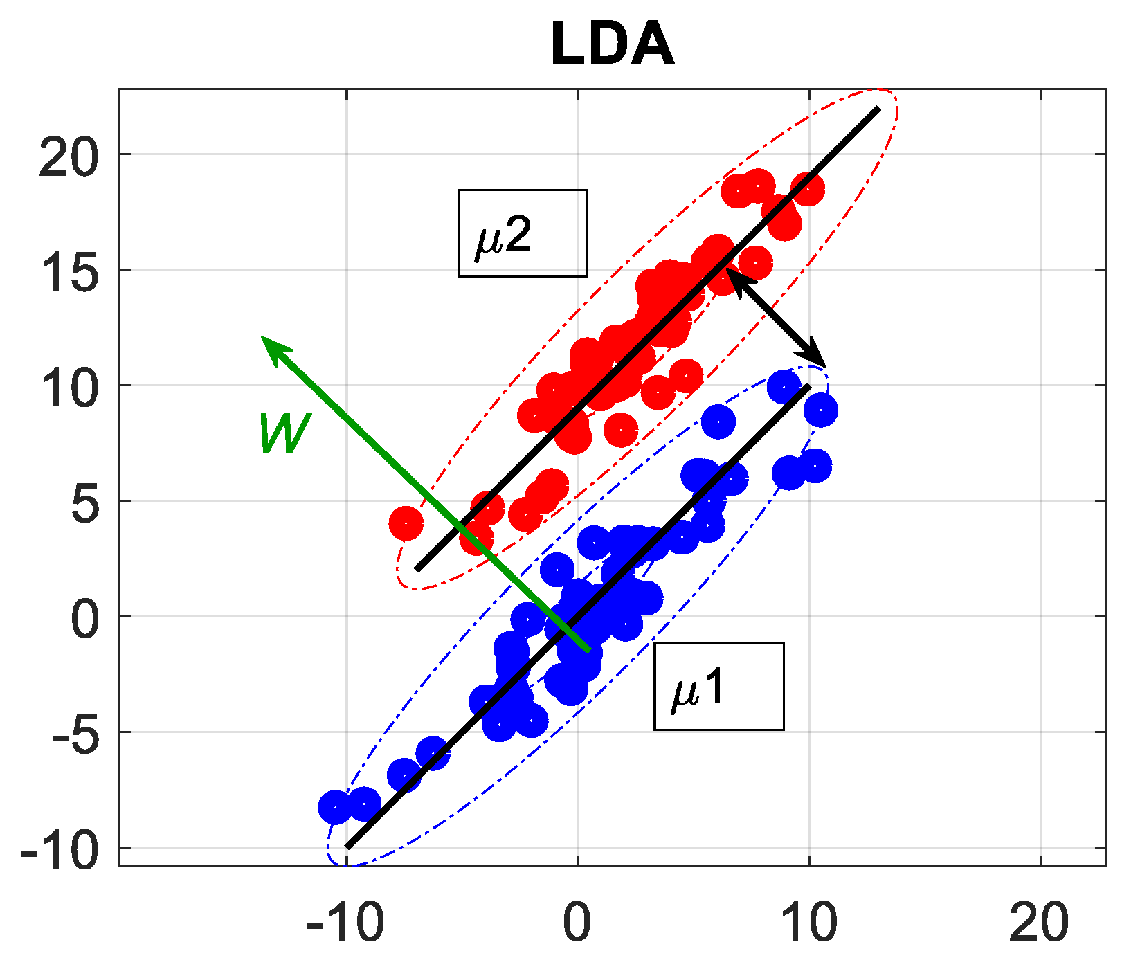
2.3. Linear Discriminant Analysis (LDA)

As introduced in Section 2.1.2, the parameter which characterizes the distance between two distributions is the effect size $d^{*}=\frac{{\mu }_1-{\mu }_2}{\sigma }$, which can be estimated from the samples as ${\widehat{d}}^{*}=\frac{E\left[x_{dam}\left]-E\right[x_{ref}\right]}{s_p}$. Fisher found a simple way to use this distance squared as a measure of separation also in case of multivariate problems, creating the linear discriminant analysis (LDA) [15]. In short, collecting the multivariate features in the rows of a matrix $X$, LDA searches for optimal linear dimensionality reduction $y=w^{\prime }X$, namely the projection $w$ which maximizes the difference between the projected class-means distance, normalized by a measure of the within-class variance (also called scatter) along the same direction. The measure of separation is then the squared effect size, also resulting as the ratio $s_{bg}^2/s_{wg}^2$, where $s_{wg}^2$ is the within groups variance and $s_{bg}^2$ is the between groups variance.

The formulation for the measure of separation of 2 groups $J\left(w\right)$ to be maximized in a multivariate feature space under the assumption of homoscedasticity is summarized in

Table 10. Linear discriminant analysis (LDA).

Scatter Matrices	Optimization of the Separation Index $\mathit{J}\left(\mathit{w}\right)$
Between class scatter matrix: $S_b={\left({\mu }_2-{\mu }_1\right)}^{\prime }\left({\mu }_2-{\mu }_1\right)$	$J\left(w\right)=\frac{w^{\prime }{S}_{b}w}{w^{\prime }{S}_{w}w}$
Within class scatter matrix: $S_w={\displaystyle {\displaystyle \sum }_{h\in C_1}{\left(x^h-{\mu }_1\right)}^{\prime }\left(x^h-{\mu }_1\right)+{\displaystyle \sum }_{k\in C_1}}{\left(x^k-{\mu }_2\right)}^{\prime }\left(x^k-{\mu }_2\right)$	$\arg \underset{w}{\max }J\left(w\right):$ $w\propto S_w^{-1}{\left({\mu }_2-{\mu }_1\right)}^{\prime }$

.

Once this maximum separation direction $w$ is found, as shown in Figure 9, a projection of the observations on this direction (i.e., a linear combination of the features) is performed, and classification can be obtained using as a threshold the average position of the projection of the two means on this single dimension. This is equivalent to finding a hyperplane able to separate the different groups in the multivariate feature space.

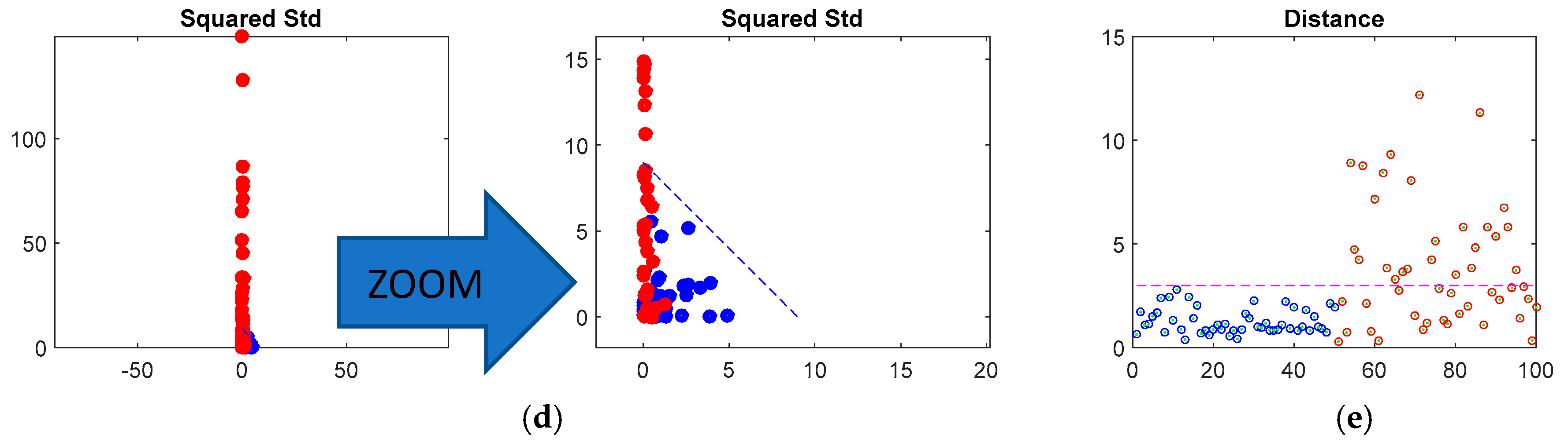
2.4. Mahalanobis Distance Novelty Detection

Damage detection is founded on the consideration that the presence of a malfunction modifies the dynamic response of the system. Hence, the data collected on a damaged machine are different from those collected on the healthy machine and can be regarded as novel. The detection of such novelty (often called anomaly detection) from a mathematical point of view corresponds to a search for the measures that are frequently higher or lower than all the others and therefore, are commonly identified with the name of outliers.

An outlier is a measure discordant from all the others and is believed to be generated by an alternate mechanism [16]. When it is possible to exclude all other possible influences (e.g., errors, latent factors like load, speed, temperature), this inconsistency can be attributed to the presence of damage. In this respect, the detection of novelty can be successfully used to perform Level 1 diagnostics. The judgment on discordancy usually depends on a measure of distance from a reference distribution, which takes the name of novelty index (NI).

The Mahalanobis distance (MD) is the optimal candidate for evaluating discordancy in a multi-dimensional space, because it is unitless and scale-invariant, and takes into account the correlation in the dataset. For a mean centred dataset $X$ the Mahalanobis distance is defined as:

$$MD\left(X\right)=\sqrt{X^{\prime }{S}^{-1}X}=\sqrt{Z^{\prime }{V}^{\prime }{S}^{-1}VZ}=\sqrt{Z^{\prime }{\mathsf{\Lambda }}^{-1}Z}=\sqrt{{{\displaystyle \sum }}_j\frac{z_j^2}{{\lambda }_j}}\equiv NI$$

(18)

Remembering the geometrical interpretation of PCA (derived in previous section, Equation (16)), it is easy to understand that the Mahalanobis distance is equivalent to a Euclidean distance on the whitened space (i.e., the feature space undergoing a rotation to PCs and a standardization). This is visualized in Figure 10, where the Mahalanobis distance is decomposed into a series of 5 simple steps.

The NIs computed with Mahalanobis distance are therefore a 1-D lossless compression of the multivariate dataset and can be compared against some objective criterion (i.e., a threshold) to judge whether the corresponding data comes from the healthy distribution. Furthermore, even for graphical purposes, these NIs are the optimal univariate dimensionality reduction tool to display possible outliers of a multivariate dataset.

Unfortunately, the procedure to generate a suitable threshold is not trivial. In this respect, probability theory and hypothesis testing offer some good suggestions.

The thresholding of the NIs is exactly equivalent to fixing a critical iso-probability ellipsoid on the multivariate normal distribution that fits the multivariate dataset. Therefore, it corresponds to a true multivariate hypothesis testing.

2.4.1. Hypothesis Testing of Outliers

The judgement of discordancy can be thought in terms of hypothesis testing to verify if a measurement is an outlier or not. For example, the Chauvenet’s criterion can be considered. The idea behind this method of assessing outliers is to find a confidence interval that should reasonably contain all $n$ values of a sample. Hence, under the assumption of a normal population $x~N\left(\mu ,\sigma \right)$, it follows that a believed outlier $x_o$ shows a statistical summary $z=\frac{x_o-\mu }{\sigma }$ which can be compared to a corresponding critical value $N{\left(0,1\right)}_{\frac{\alpha }{2}}$ for a significance $\alpha =\frac{1}{n}$. In other words, the value which is exceeded just once every $n$ values is used as critical, so that:

$$\mu -\sigma N_{\left(0,1\right),\frac{1}{2n}}\le x_o\le \mu +\sigma N_{\left(0,1\right),\frac{1}{2n}}$$

(19)

The other way around, comparing $2\min \left(\mathrm{Pr}\left(Z\ge z|H_0\right),\mathrm{Pr}(Z\le z|H_0)\right)$, namely the p-value of the summary $z=\frac{x_o-\mu }{\sigma }$, to the significance $\alpha =\frac{1}{n}$, an equivalent test for the hypothesis $H_0:x_o\mathrm{is}\mathrm{not}\mathrm{an}\mathrm{outlier}$ can be found. If the p-value is less than or equal to the significance, $H_0$ is rejected. Obviously, substituting $\mu$ and $\sigma$ with their sample estimates, the same formula can be used under the assumption of large $n$. Unfortunately, in many cases, this assumption does not hold, so that compensation is needed. Furthermore, Chauvenet’s criterion works in univariate cases. To find a corresponding multivariate hypothesis test, the Mahalanobis distance can be exploited, as it enables to generalize these considerations.

If the assumption of multivariate normality holds for the original multivariate distribution of the features, and the true covariance matrix $\Sigma$ and the mean value vector $\mu$ are known, the sum of squares $N{I}^2$ is distributed as a perfect ${\chi }_d^2$. Given $N{I}^2~{\chi }_{\left(d\right)}^2$ the corresponding $1-\alpha$ confidence interval results:

$$N{I}^2={\left(X-\mu \right)}^{\prime }{\Sigma }^{-1}\left(X-\mu \right)\le {\chi }_{\left(d\right),\alpha }^2$$

(20)

Due to [22], it is easy to correct this formulation for the use of the sample estimates $\overline{x_n}$ and $S_n$ which are not independent from the observations for $n$ small. Hence, the so-called Wilks’s critical value is given

$$N{I}^2={\left(X-\overline{x_n}\right)}^{\prime }{S}_n{}^{-1}\left(X-\overline{x_n}\right)\le \frac{d{\left(n-1\right)}^2{F}_{\left(d,n-d-1\right),\frac{\alpha }{n}}}{n\left(n-d-1+d{F}_{\left(d,n-d-1\right),\frac{\alpha }{n}}\right)}$$

(21)

where $F_{\left(d,n-d-1\right)}$ is the Fisher–Snedecor distribution with degrees of freedom $d$ and $n-d-1$.

Overall, keeping the same significance $\alpha =1/n$, it is possible to summarize the two confidence intervals in a single criterion holding for any $n$ (either small or large):

$$NI\le \min \left(\sqrt{{\chi }_{\left(d\right),\frac{1}{n}}^2},\sqrt{\frac{d{\left(n-1\right)}^2{F}_{\left(d,n-d-1\right),1-\frac{1}{n^2}}}{n\left(n-d-1+d{F}_{\left(d,n-d-1\right),1-\frac{1}{n^2}}\right)}}\right)$$

(22)

These considerations can be easily proved through Monte Carlo repetitions on a multivariate Gaussian distribution, as suggested by Worden [16]:

• Draw a sample of $n$ observations randomly generated from a $d$-dimensional standard normal distribution,
• Compute the deviation of each observation in terms of distance from the centroid i.e., the NI,
• Save the maximum deviation and repeat the draw for $m$ times.

The result of such operation is a collective whose distribution can be studied exploiting the extreme value theory (EVT), a branch of statistics dealing with extreme deviations from the mean.

In EVT [23,24] it is well known that, in the limit for the number of repetitions $m$ tending to infinity, the induced distribution of the maxima can take 3 shapes only: Gumbel, Weibul or Frechet. Furthermore, the Gaussian distribution is known to fall in the domain of attraction of the Gumbel. The Gumbel cdf is given by:

$$G(z|{\mu }_g,{\sigma }_g)=e^{-e^{-\frac{z-{\mu }_g}{{\sigma }_g}}}$$

(23)

where the location parameter ${\mu }_g$ is the mode of the distribution, while ${\sigma }_g$ is the scale (or dispersion) parameter. Following von Mises’s theorem [25], it can be proved that the ideal asymptotical location parameter for the NIs as a function of the sample numerousness $n$ is exactly:

$${\mu }_g\left(n\right)=\sqrt{{\chi }_{\left(d\right),\frac{1}{n}}^2}$$

(24)

These theoretical values can be easily compared to their corresponding simulated values ${\widehat{\mu }}_g^2$ coming from the Monte Carlo repetition. As shown in Figure 11b, Equation (22) is a very good approximation, but in a mid-range of $n$, the error can be quite large in percentage, so that it can be safer to use Monte Carlo simulations, which are becoming every day more inexpensive in terms of computational times as the average computer power is growing.

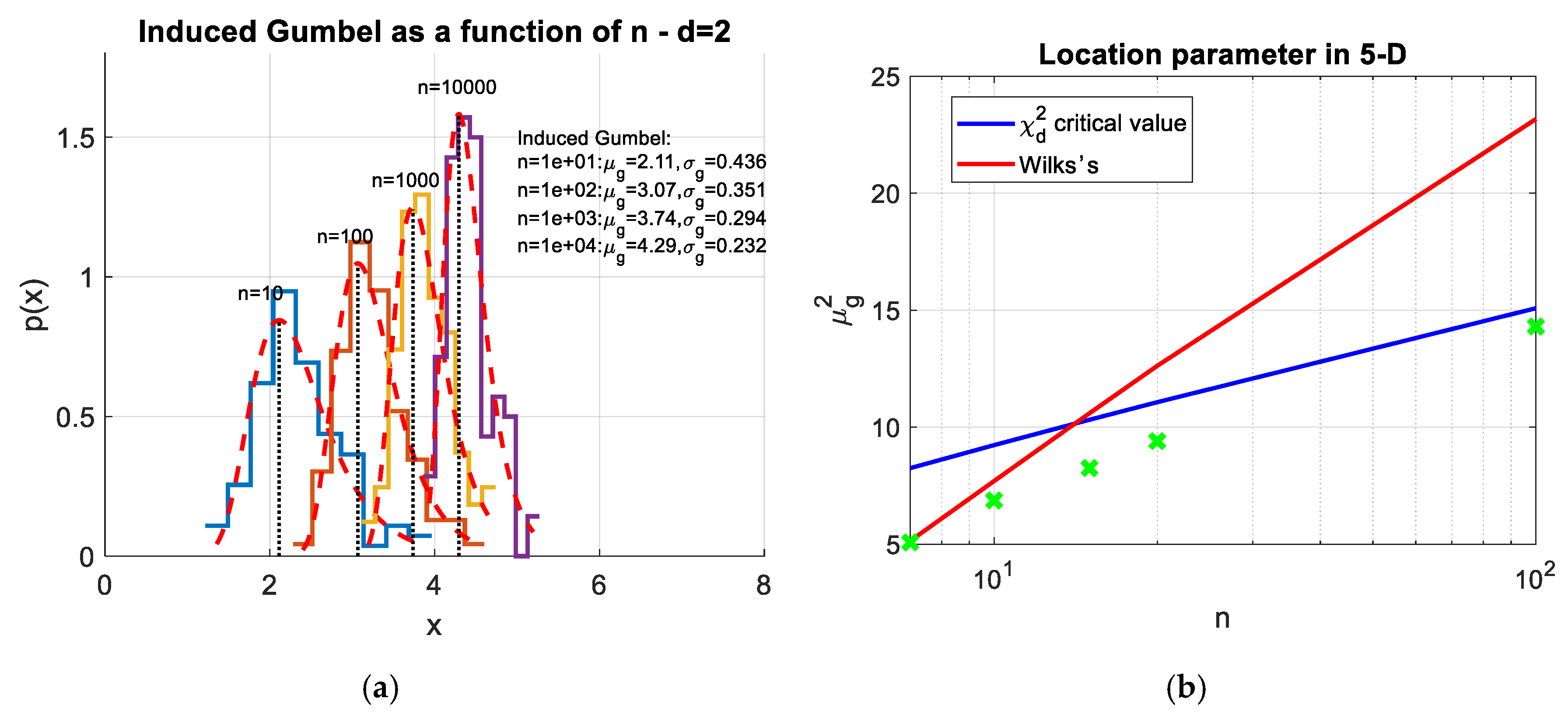
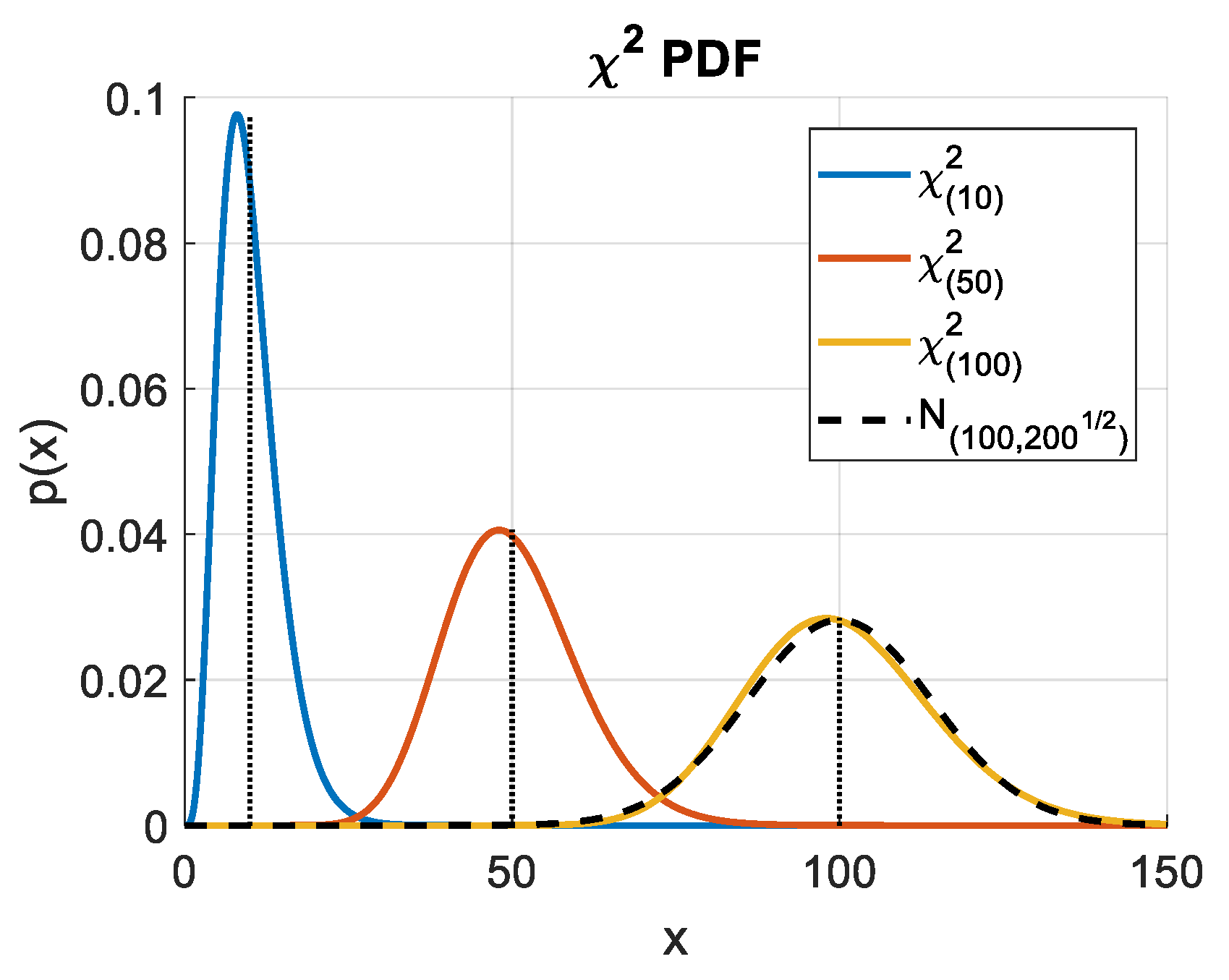
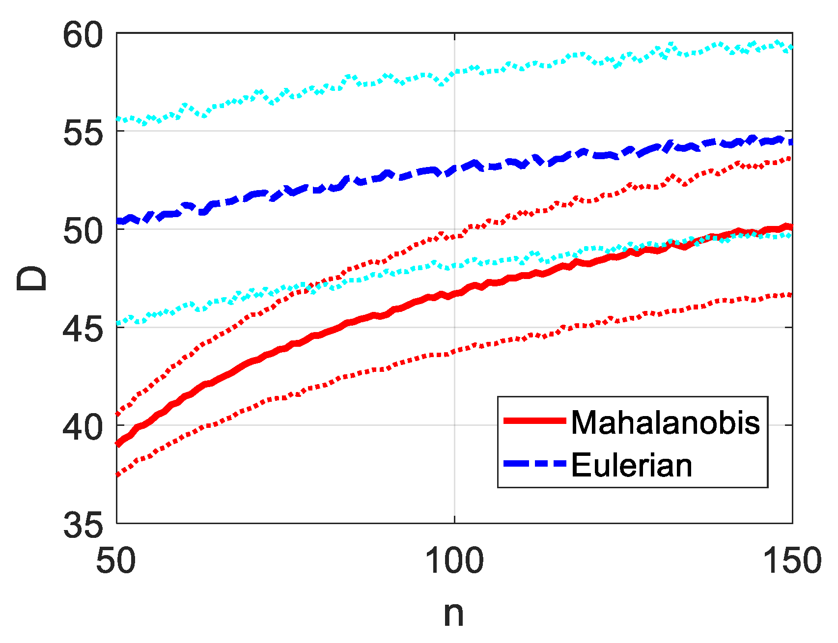
2.4.2. The Curse of Dimensionality

Considerations about the so-called curse of dimensionality can be derived from the analysis in Section 2.4.1. When the space dimensionality increases in fact, the volume of the space becomes larger quickly that the available data is usually insufficient to fill it and the data-cloud appears to be sparse, eroding the confidence on statistical estimates. Moreover, comparing the volume of a hypercube to the volume of the inscribed hypersphere, it is possible to derive that the ratio $V_{h-sphere}/V_{h-cube}$ tends to $0$ as $d\to \infty$, while the distance between the centre and the corners increases without any bound with $d$. Therefore, the high-dimensional unit hypercube is said to consist almost entirely of the corners with almost no middle. This space density deformation is highlighted also by the ${\chi }^2$ distribution shape. As illustrated in Figure 12, in fact, most of the $d$-cube volume concentrates near the surface of a sphere of radius $\sqrt{d}$ and the limiting distribution of the ${\chi }_{\left(d\right)}^2$ for an increasing $d$ (i.e., $d>50$) can be proved to be the normal $N_{\left(d,\sqrt{2d}\right)}$.

As the volume of the space increases as a power of $d$, $n$ should do the same to ensure the same filling of space and a consequent equal reliability in estimates of mean vector and covariance matrix. At a DOE stage, considerations about the selection of a proper sample size $n$ are fundamental. The problem of ensuring a confident estimate of the covariance matrix is approached in [26] for the simplified case of a diagonal covariance. Obviously, the result is that a sharp increase in $n$ is prescribed as $d$ increases, so that when $d$ is very large, it is likely that $n$ will be too big to be matched. Another method based on Monte Carlo repetitions is proposed in [12], based on the considerations about the geometric interpretation of the Mahalanobis distance introduced hereinbefore. In particular, the MD was proved to be equivalent to a Eulerian distance on the standardized principal component space. In this respect then, repeating $m=1000$ draws of size $n$ from a multivariate Gaussian of dimension $d=30$ (of interest in this work) the Eulerian distance can be compared to the Mahalanobis distance obtained by estimating the sample mean (whose expected value is the null vector) and the sample covariance matrix (whose expected value is the identity matrix). Hence, the Mahalanobis distance is expected to be equal to the Euclidean, but because of the mean and covariance estimation errors, the two values start diverging when $n$ is not large enough to fill the $d$-dimensional space. Fixing $d=30$ and letting $n$ increase, it is possible to compute some statistics on the $m$ values produced by MC repetition. In particular, the mean value of the two distances and the $\pm \sigma$ confidence interval are given in Figure 13. In accordance with this analysis, $n=100$ is selected in this work. Obviously a $n<80$ would produce unreliable results.

2.4.3. Mahalanobis Distance and Confounding Influences

Hereinbefore, it was stated that the distance from a population centroid can be used as a measure of discordancy. Moreover, this novelty can be considered induced by an alternative mechanism, such as damage when it is possible to exclude all other possible influences like measurement errors, operational conditions (e.g., speed, load) and environmental conditions (e.g., temperature, humidity). These factors are often latent (not measured), but when they can freely change in time, their variation must be investigated, as it appears to be a confounding influence for damage detection. Generally speaking, when this influence is strong, it can be proved to be a main source of variability in the dataset, so that it is pictured by PCA in one of the first (or most probably the first) principal component [21,27]. Assuming a generic influence on the selected features can lead to a strong linear or at least a quasi-linear relationship among the features, this can be captured by a principal component, the removal of which becomes helpful in highlighting the damage influence. Nevertheless, in this work, coherently with the belief that a lossless analysis is much more conservative (and then safer), this procedure is not taken into account. Furthermore, remembering again the geometrical interpretation of PCA and Mahalanobis distance: $NI=\sqrt{{{\displaystyle \sum }}_j\frac{z_j^2}{{\lambda }_j}}$, it is obvious how the influence of the components with larger variance (i.e., the first components and then also the confounding factors) is mitigated by their normalization on the corresponding eigenvalue. This means that the Mahalanobis distance-based novelty indices implicitly compensate for strong, quasi-linear confounding effects [4,12].

3. The Results

The dataset collecting the extracted features described in Section 1.4 was processed using the algorithms presented in Section 2. At first, a single speed-load condition was selected. In particular, referring to Table 3, the results for condition 12 ($280\mathrm{Hz},1800\mathrm{N}$) and condition 3 ($90\mathrm{Hz},1400\mathrm{N}$) are reported. They are respectively the best and the worst conditions in diagnostic terms. The three different 1-D dimensionality reductions (PCA, LDA and MD, introduced in Section 2.2, Section 2.3 and Section 2.4 respectively) and the corresponding diagnostic performance are reported in Figure 14 and Figure 15, summarizing conditions 12 and 3.

In Figure 14 and Figure 15a–f, the 1-D reductions are shown together with the empirical pdf of the healthy and damaged distributions. For LDA (Figure 14 and Figure 15c), a separating threshold midway from the two distributions is also added. The same is done for the Mahalanobis’ NIs, for which the Monte Carlo threshold described in Section 2.4.1 is reported. In Figure 14 and Figure 15g, the ROC curves defining the performances of the three dimensionality reductions are represented. The Mahalanobis’ NIs threshold is highlighted and compared to a 5% significance threshold, which is common for general-purpose hypothesis testing. In Figure 14 and Figure 15h, for the sake of investigation and visualization, the data is projected on the plane formed by the first 2 principal components, where the Fisher’s LDA direction $w$ is also reported.

As is clearly noticeable in Figure 14, for both LDA and MD, the separation is perfect, even with LDA, the different damaged conditions are indistinguishable, while in the second case, with MD, the distance appears more consistent with the damage level. Figure 14g, summarizing the 1-D classification with the ROC curves, confirms the lower performance of the PCA compression. This can be explained focusing on the projection on the plane formed by the first 2 principal components. From Figure 14h, it is clear that the direction of maximum separation $w$ is much nearer to the second principal component rather than the first, which pictures mainly the diversity among the different damages, and not the distance between the damaged clouds and the healthy condition.

Analogous considerations can be obtained by focusing on Figure 15, but the recognition of the damaged condition becomes, in this case more difficult, in particular for 3A damage (the smallest Inner Race damage—$150\mathsf{\mu }\mathrm{m}$) and for 5A damage (the mid Rolling Element damage—$250\mathsf{\mu }\mathrm{m}$). It is easy to notice that the damaged and the healthy distributions get nearer (compare Figure 14b,d,f and Figure 15b,d,f), highlighting a reduction of the effect size of the test which causes a reduction in the test’s power (higher probability of missed alarms). Indeed, in Figure 15g, the ROC suggests that the missed alarms probability can increase up to 8% when the Monte Carlo threshold, ensuring no false alarms is used with MD and up to 18% for ensuring the same null false alarm rate using LDA.

This highlights how the threshold selection, when the effect size is not high enough, is always a trade-off between the minimization of false alarms (FPR in the ROC) and missed alarms (1-TPR).

In order to assess the performance of the classifiers when the speed and load are not constant, the analysis was repeated grouping conditions 5, 6, 7 and 8 which feature a constant speed of $180\mathrm{Hz}.$ The load is increased ($0,1000,1400,1800$ N respectively) and conditions 2, 6, 10, 14 and 17 are measured for the same constant load of $1400$N, while the speed increases ($90,180,280,370,470\mathrm{Hz}$ respectively). As reported in Figure 16, in both cases the performance of all the classifiers was reduced, but the MD proved to be still the most reliable, as at a significance of 5% (high confidence on the recognition of the healthy condition), it is able to keep a power always greater than 80% (high sensitivity to damage).

When both speed and load variability was accounted (Figure 17), the damage sensitivity decreased. Even MD power fell to approximately 70%, so that 3 times out of ten, damage was missed. In this regard, the confusion matrix reported in

Table 11. MD confusion matrix for the whole dataset involving both speed and load variability. The 5% significance threshold highlighted in Figure 17 is used, as highlighted by the 0A false alarms rate of $5\%$.

		True Class
		0A	1A	2A	3A	4A	5A	6A
Classified	Healthy	95	9	52	64	0	32	26
	Damaged	5	91	48	36	100	68	74

helps in understanding that this percentage was not uniform across the different damages. The largest 4A and 1A were almost perfectly recognized using the 5% significance threshold (i.e., accepting a false alarms rate of $5\%$). Hence, even if the detection of incipient damage (2A, 3A, 5A, 6A) became harder in case of speed and load variability, the damage presence was still detected in case of developed damages (1A, 4A). (N.B. notice that 4A and 1A damages are not large in absolute terms, as they correspond to indentations of size $450\mathsf{\mu }\mathrm{m}$).

4. Discussion

The scope of the paper was to study the problem of bearing damage detection from a hypothesis testing point of view. This allowed the study to extend the ideas of confidence, effect size, and power to the subject of machine diagnostics via statistical analyses, such as classification and novelty detection. From a practical point of view, the first fundamental target of diagnostics is the detection of incipient damage, that is, the recognition of a damaged condition from the available measurements, and in this case, coming from accelerometers (i.e., vibration monitoring). The performance of such a recognition is usually evaluated in terms of false alarms rates (or false positive rate), which measures the statistical significance at which the healthy condition is identified, and missed alarms rates (that is 1—True Positive Rate) which gives the statistical confidence at which a damaged condition is recognized (i.e., 1—power). Obviously, in the ideal case, the scope is to find a threshold which allows a perfect recognition, implying zero false alarms and zero missed alarms at the same time. Unfortunately, this is not always possible as, in common cases, the effect size (i.e., the distance of the healthy distribution from the damaged distribution) is not high enough, therefore, a trade-off between the two alarms is an obligation. A high number of triggered false alarms can erode the confidence of the damage detection and, at the same time, a missed indication of damage can bring serious economic and life-safety implications, therefore, the optimization of the threshold can be effectively performed only by an expert of the particular industrial field.

In any case, these alarm rates are not independent from the selection of the number of samples to be considered, the features to be involved and the algorithms used for performing the multivariate pattern recognition (classification of novelty detection). This paper also proved that the common time series features can be used to perform damage detection of bearings, even when the conditions are not perfectly stationary, as speed and load variations can be compensated in a satisfactory way for a fast, online, first order analysis. Furthermore, this work underlined that among alternative 1-D dimensionality reductions, the Mahalanobis distance is the best in highlighting a damaged condition, as it performs a lossless compression of the multivariate dataset, unlike LDA and PCA (reduction to the first principal component).

Alternative approaches to cope with multivariate datasets are obviously possible. In particular, in order to improve the compensation of latent factors (e.g., operational conditions, temperature, etc.), non-linear approaches can be used involving, for example, neural networks (as found in [28,29]). Nevertheless, the Mahalanobis distance can be a good starting point as it proved to perform quite well with variable operating conditions (when their effect is to produce quasi linear relations of the features).

Finally, the curse of dimensionality must always be accounted for in the selection of a proper number of samples for training the algorithms, as it is fundamental to ensure reliability, robustness and statistical significance of the results.

5. Conclusions

In this analysis, statistical and hypothesis testing considerations were used to perform damage detection in terms of classification (supervised) or novelty detection (semi-supervised). The strategy was reducing the dimensionality of a multivariate dataset to a single variable which summarizes the relevant health information. Simple time features were extracted from the raw acceleration measurements coming from the DIRG test rig conceived for high speed aeronautical bearings [12]. These formed a 30-dimensional dataset which was later compressed to a 1-D index. Three algorithms were introduced for performing such compression. The simplest was based on PCA. The dataset was projected on the first principal component computed from the healthy set (during calibration), but this proved to be a lossy compression, as part of the health information was removed together with the remaining principal components. Fisher’s LDA was then introduced as it is able to find the direction $w$ which maximizes the separation of the healthy and the damaged clouds (which are both used to train the algorithm). This improvement proved to be very effective, but still some part of the health information related to the direction in the feature space may be lost. In particular, a phenomenon developing in a direction orthogonal to $w$ can never be highlighted. Finally, a lossless alternative was found in the Mahalanobis-distance-based novelty detection. A univariate test on the Mahalanobis distance novelty index (MD-NI) leading to a confidence interval based on a single threshold (i.e., a critical value) is equivalent to a multivariate test for outliers based on a corresponding critical ellipsoid in the multidimensional feature space. Even the direction information is preserved in this case, so that optimal behavior is expected. This was verified by the analysis carried out in this work. Furthermore, the tests also confirmed the theoretical conjecture according to which MD is able to compensate for latent confounding influences, such as variable operational conditions (speed and load).

The high confidence and high sensitivity to damage which can be reached by MD-NI are unmatched and make the here-proposed methodology suitable for integration in condition based maintenance regimes based on vibration monitoring. The results are very interesting also in terms of speed, simplicity and full independence from human interaction, making the methodology suitable for real time implementation. The work concluded with final considerations about the curse of dimensionality and the minimum sample size which can ensure statistical confidence. This is fundamental at the design of experiment (DOE) stage to foster the reliability of the method.

In conclusion, the analysed methodology can be considered successful in fostering the condition based maintenance of machines through vibration monitoring.

References

1. Farrar, C.R.; Doebling, S.W. Damage Detection and Evaluation II. In Modal Analysis and Testing; Silva, J.M.M., Maia, N.M.M., Eds.; NATO Science Series (Series E: Applied Sciences); Springer: Dordrecht, The Netherlands, 1999; ISBN 978-0-7923-5894-7. [Google Scholar]
2. Rytter, A. Vibration Based Inspection of Civil Engineering Structures. Ph.D. Thesis, University of Aalborg, Aalborg, Denmark, May 1993. [Google Scholar]
3. Worden, K.; Dulieu-Barton, J.M. An overview of intelligent fault detection in systems and structures. Struct. Health Monit. 2004, 3, 85–98. [Google Scholar] [CrossRef]
4. Deraemaeker, A.; Worden, K. A comparison of linear approaches to filter out environmental effects in structural health monitoring. Mech. Syst. Signal Process. 2018, 105, 1–15. [Google Scholar] [CrossRef]
5. Jardine, A.K.S.; Lin, D.; Banjevic, D. A review of machinery diagnostics and prognostics implementing condition-based maintenance. Mech. Syst. Signal Process. 2006, 20, 1483–1510. [Google Scholar] [CrossRef]
6. Zhang, W.; Zhou, J. Fault Diagnosis for Rolling Element Bearings Based on Feature Space Reconstruction and Multiscale Permutation Entropy. Entropy 2019, 21, 519. [Google Scholar] [CrossRef]
7. You, L.; Fan, W.; Li, Z.; Liang, Y.; Fang, M.; Wang, J. A Fault Diagnosis Model for Rotating Machinery Using VWC and MSFLA-SVM Based on Vibration Signal Analysis. Shock Vib. 2019, 2019, 1908485. [Google Scholar] [CrossRef]
8. Randall, R.B.; Antoni, J. Rolling Element Bearing Diagnostics—A Tutorial. Mech. Syst. Signal Process. 2011, 25, 485–520. [Google Scholar] [CrossRef]
9. Antoni, J.; Griffaton, J.; Andréc, H.; Avendaño-Valencia, L.D.; Bonnardot, F.; Cardona-Morales, O.; Castellanos-Dominguez, G.; Paolo Daga, A.; Leclère, Q.; Vicuña, C.M.; et al. Feedback on the Surveillance 8 challenge: Vibration-based diagnosis of a Safran aircraft engine. Mech. Syst. Signal. Process. 2017, 97, 112–144. [Google Scholar] [CrossRef]
10. Antoni, J.; Randall, R.B. Unsupervised noise cancellation for vibration signals: Part I and II—Evaluation of adaptive algorithms. Mech. Syst. Signal Process. 2004, 18, 89–117. [Google Scholar] [CrossRef]
11. Caesarendra, W.; Tjahjowidodo, T. A Review of Feature Extraction Methods in Vibration-Based Condition Monitoring and Its Application for Degradation Trend Estimation of Low-Speed Slew Bearing. Machines 2017, 5, 21. [Google Scholar] [CrossRef]
12. Daga, A.P.; Fasana, A.; Marchesiello, S.; Garibaldi, L. The Politecnico di Torino rolling bearing test rig: Description and analysis of open access data. Mech. Syst. Signal Process. 2019, 120, 252–273. [Google Scholar] [CrossRef]
13. Sikora, M.; Szczyrba, K.; Wróbel, Ł.; Michalak, M. Monitoring and maintenance of a gantry based on a wireless system for measurement and analysis of the vibration level. Eksploat. Niezawodn. 2019, 21, 341. [Google Scholar] [CrossRef]
14. Jolliffe, I.T. Principal Component Analysis; Springer: New York, NY, USA, 2002. [Google Scholar]
15. Bishop, C. Pattern Recognition and Machine Learning; Springer: New York, NY, USA, 2006; ISBN 978-0-387-31073-2. [Google Scholar]
16. Worden, K.; Manson, G.; Fieller, N.R.J. Damage detection using outlier analysis. J. Sound Vib. 2000, 229, 647–667. [Google Scholar] [CrossRef]
17. Von Mises, R. Probability, Statistics, and Truth, 2nd rev. English ed.; Dover Publications: New York, NY, USA, 1981; ISBN 0-486-24214-5. [Google Scholar]
18. Holman, J.P.; Gajda, W.J. Experimental Methods for Engineers; McGraw-Hill: New York, NY, USA, 2011; ISBN 10: 0073529303. [Google Scholar]
19. Daniel, W.W.; Cross, C.L. Biostatistics: A Foundation for Analysis in the Health Sciences; Wiley: Hoboken, NJ, USA, 2012; ISBN 13: 978-1118302798. [Google Scholar]
20. Howell, D.C. Fundamental Statistics for the Behavioral Sciences, 8th ed.; Cengage Learning: Boston, MA, USA, 2013; ISBN 13: 978-1285076911. [Google Scholar]
21. Yan, A.M.; Kerschen, G.; De Boe, P.; Golinval, J.C. Structural damage diagnosis under varying environmental conditions—Part I: A linear analysis. Mech. Syst. Signal Process. 2005, 19, 847–864. [Google Scholar] [CrossRef]
22. Penny, K.I. Appropriate critical values when testing for a single multivariate outlier by using the Mahalanobis distance. J. Royal Stat. Soc. Series C (Appl. Stat.) 1996, 45, 73–81. [Google Scholar] [CrossRef]
23. Worden, K.; Allen, D.W.; Sohn, H.; Farrar, C.R. Damage detection in mechanical structures using extreme value statistics. SPIE 2002. [Google Scholar] [CrossRef]
24. Toshkova, D.; Lieven, N.; Morrish, P.; Hutchinson, P. Applying Extreme Value Theory for Alarm and Warning Levels Setting under Variable Operating Conditions. Available online: https://www.ndt.net/events/EWSHM2016/app/content/Paper/293_Filcheva_Rev4.pdf (accessed on 5 June 2019).
25. Takahashi, R. Normalizing constants of a distribution which belongs to the domain of attraction of the Gumbel distribution. Stat. Probab. Lett. 1987, 5, 197–200. [Google Scholar] [CrossRef]
26. Gupta, P.L.; Gupta, R.D. Sample size determination in estimating a covariance matrix. Comput. Stat. Data Anal. 1987, 5, 185–192. [Google Scholar] [CrossRef]
27. Yan, A.M.; Kerschen, G.; De Boe, P.; Golinval, J.C. Structural damage diagnosis under varying environmental conditions—Part II: Local PCA for non-linear cases. Mech. Syst. Signal Process. 2005, 19, 865–880. [Google Scholar] [CrossRef]
28. Deraemaeker, A.; Worden, K. New Trends in Vibration Based Structural Health Monitoring; Springer Science & Business Media: Berlin/Heidelberg, Germany, 2012; ISBN 978-3-7091-0399-9. [Google Scholar]
29. Arnaiz-González, Á.; Fernández-Valdivielso, A.; Bustillo, A.; López de Lacalle, L.N. Using artificial neural networks for the prediction of dimensional error on inclined surfaces manufactured by ball-end milling. Int. J. Adv. Manufact. Technol. 2016, 83, 847–859. [Google Scholar] [CrossRef]
Figure 1. The experimental setup, the triaxial accelerometers location (A1 and A2) and orientation (a) Constructive parts; (b) Bearings and accelerometers location.
Information 10 00204 g001
Figure 2. The considered dataset after features extraction. The black dotted lines divide the different damage conditions (0A to 6A). For each, the 100 observations for the 17 speed and loads conditions are plotted sequentially.
Information 10 00204 g002
Figure 3. The damage (a conical indentation) on the rolling element as obtained through a Rockwell tool (a) and its evolution after 19 h at various load and speed conditions (b). Dimensions in mm.
Information 10 00204 g003
Figure 4. One or two tail hypothesis testing principle: significance α (limit for the p-value) and critical value(s) of the confidence interval highlighted (a) single sided; (b) double sided.
Information 10 00204 g004
Figure 5. Visual representation of the hypothesis test of the difference between two population means—the critical values are highlighted together with the corresponding significance in terms of tail areas (in cyan).
Information 10 00204 g005
Figure 6. The power of a two population means test—(a) a visualization of the significance α and of the power 1 β for a particular case—(b) the power (under assumption of normality) as a function of t * which depends on the effect size μ 1 μ 2 σ = d and the sample size n .
Information 10 00204 g006
Figure 7. Receiver Operating Characteristic (ROC) as a function of the threshold (Gaussian distributions). (a) graphical summary of the table of type I and type II errors in yellow (Table 9). (b) ROC for binary classification with different effect sizes d   * and the position of the 95% critical value (black dotted). For d   *   = 0.2 the performance is very poor as the ROC is near to the 1st–3rd quadrant bisector (random classifier).
Information 10 00204 g007
Figure 8. Visualization of the principal component analysis (PCA) principle for a 2D case—geometric interpretation.
Information 10 00204 g008
Figure 9. Visualization of the LDA idea for a 2 groups case. 2D case geometric interpretation.
Information 10 00204 g009
Figure 10. Mahalanobis equivalent procedure on a 2D simplified plane, for 2 simulated normal classes (blue: reference, red: novel). Notice that the Centring (a) and Standardization (c) of the space is unique and based on the reference set alone. All the novel acquisitions are later mapped to the same space. (a) Data centred on reference condition; (b) Rotated according to PCs; (c) Standardized;(d) Squared components: non-linear space transform; (e) Distance from centre (origin).
Information 10 00204 g010aInformation 10 00204 g010b
Figure 11. (a) Several different Induced Gumbel distributions for the maxima arising from a bivariate standard normal, as a function of n, for m = 100 Monte Carlo Repetitions. (b) Monte Carlo sampling from a 5-dimensional multivariate normal with random mean and covariance matrix. The μ ^ g 2 values obtained from fitting a Gumbel (green dots) are compared to the theoretical μ g 2 ( n ) critical values form χ 2 and Wilk’s criteria.
Information 10 00204 g011
Figure 12. Three χ 2 distributions for an increasing number of dofs. The χ 100 2 is compared to the asymptotical tendency distribution N ( 100 ,   200 ) . The asymptotical means are highlighted as black dotted lines. Notice that increasing the dofs, the distribution concentrates around the asymptotical mean.
Information 10 00204 g012
Figure 13. Averages of the estimated Mahalanobis distances (red) and true Eulerian distances (blue) for the Maxima of a 30 -dimensional multivariate Gaussian, as a function of the sample numerousness n , considering 1000 Monte Carlo repetitions. ±σ confidence intervals of the estimates are also given in cyan (Eulerian) and red (Mahalanobis).
Information 10 00204 g013
Figure 14. Results for for condition 12 ( 280   Hz ,   1800   N ) alone: (a,c,e) the 3 different dimensionality reductions; (b,d,f) the corresponding empirical pdf for the healthy condition (blue) and for the 6 damage conditions (red). The x axis represents the 100 observations for each of the different damage conditions (ordered from 0A to 6A) which are separated by the black dotted lines. (g) ROC curves for the three 1-D reductions. The 5% significance threshold values are highlighted with the black circles; the black x denotes the position of the novelty index (NI) threshold computed according to the MC repetition introduced in Section 2.4.1—in magenta in (h) The 2-D PCA visualization of the dataset (condition 12) and the LDA direction w .
Information 10 00204 g014aInformation 10 00204 g014b
Figure 15. Results for condition 3 ( 90   Hz ,   1400   N ) alone (a,c,e) the 3 different dimensionality reductions; (b,d,f) the corresponding empirical pdf for the healthy condition (blue) and for the 6 damage conditions (red). The x axis represents the 100 observations for each of the different damage conditions (ordered from 0A to 6A) which are separated by the black dotted lines. (g) ROC curves for the three 1-D reductions. The 5% significance threshold values are highlighted with the black circles; the black x denotes the position of the NI threshold computed according to the MC repetition introduced in Section 2.4.1—in magenta in (h) The 2-D PCA visualization of the dataset (condition 12) and the LDA direction w .
Information 10 00204 g015aInformation 10 00204 g015b
Figure 16. (a) ROC curves for the three classifications considering constant speed ( 180   Hz ) but variable load ( 0 ,   1000 ,   1400 ,   1800   N )—conditions 5 to 8. (b) ROC curves for the three classifications considering constant load ( 1400   N ) but variable speed ( 90 ,   180 ,   280 ,   370 ,   470   Hz )—conditions 2, 6, 10, 14, 17.The 5% significance threshold values are highlighted with the black circles; the black x denotes the position of the NI threshold computed according to the MC repetition introduced in Section 2.4.1.
Information 10 00204 g016
Figure 17. ROC curves for the three classifications considering the whole dataset involving both speed and load variability (all the 17 conditions in Table 3). The 5% significance threshold values are highlighted with the black circles; the black x denotes the position of the NI threshold computed according to the MC repetition introduced in Section 2.4.1.
Information 10 00204 g017