Article

An Efficient Image Reconstruction Framework Using Total Variation Regularization with Lp-Quasinorm and Group Gradient Sparsity

School of Physics and Information Engineering, Minnan Normal University, Zhangzhou 363000, China
*
Author to whom correspondence should be addressed.
Information 2019, 10(3), 115; https://doi.org/10.3390/info10030115
Submission received: 22 February 2019 / Revised: 12 March 2019 / Accepted: 13 March 2019 / Published: 16 March 2019
(This article belongs to the Section Information Processes)

Abstract

:
The total variation (TV) regularization-based methods are proven to be effective in removing random noise. However, these solutions usually have staircase effects. This paper proposes a new image reconstruction method based on TV regularization with Lp-quasinorm and group gradient sparsity. In this method, the regularization term of the group gradient sparsity can retrieve the neighborhood information of an image gradient, and the Lp-quasinorm constraint can characterize the sparsity of the image gradient. The method can effectively deblur images and remove impulse noise to well preserve image edge information and reduce the staircase effect. To improve the image recovery efficiency, a Fast Fourier Transform (FFT) is introduced to effectively avoid large matrix multiplication operations. Moreover, by introducing accelerated alternating direction method of multipliers (ADMM) in the method to allow for a fast restart of the optimization process, this method can run faster. In numerical experiments on standard test images sourced form Emory University and CVG-UGR (Computer Vision Group, University of Granada) image database, the advantage of the new method is verified by comparing it with existing advanced TV-based methods in terms of peak signal-to-noise ratio (PSNR), structural similarity (SSIM), and operational time.

1. Introduction

Owing to the influence of sensing equipment, imaging systems, environmental conditions, and human factors, digital images are usually subject to a certain degree of degradation such as image blur, image noise, and partial image information loss. It is widely assumed that the convolution of a clear original image with a blur kernel gives a blurred image, which will further turn into a degraded image when interfered with by noise. Common types of blur kernels are Gaussian blur kernel, motion blur kernel, and average blur kernel [1]. According to the distribution condition of probability density function (PDF) of their amplitude, noises are classified into Gaussian noise, impulse noise, Rayleigh noise, exponential noise, gamma noise, etc. [1]. Designing image optimization models and proposing efficient algorithms by using degraded images and some prior information properly to reconstruct clear images is of great importance to the advanced postprocessing of images.
Reconstructing a degraded image to the original image is an inverse problem. Seeking solutions to an inverse problem is ill-posed in the sense that there is a lack of any solution or a lack of a unique, stable solution [2,3]. To deal with such a type of ill-posed problem, image reconstruction based on regularization is an effective method. In a regularization model, the image reconstruction function consists of two parts: a fidelity term and a regularization term. The fidelity term can be obtained from a priori information of the image. Given that an imaging process may be affected by different types of degradation factors, the fidelity terms may be modeled differently. However, the use of a different regularization term in a regularization function has a large effect on the quality of reconstructed images. The relative significance of fidelity and regularization terms can be adjusted by regularization parameters.
The selection of a regularization function is of great research interest in the field of image processing, and many effective models have been proposed by scholars for different applications [4,5,6,7]. Phillips [8] and Tikhonov [9] proposed smooth regularization terms, which were derived from the L2-norm and referred to as the Tikhonov regularization method. As a classic regularization method, the Tikhonov regularization method has the advantage of calculation simplicity but usually leads to oversmoothing of the edges of images. In 1992, Rudin, Osher, and Fatemi [10] pioneered the total variation (TV) regularization method, also known as the ROF model, which can well preserve image edge features and has attracted widespread attention in the image denoising field.
The TV models are divided into the anisotropic total variation (ATV) model and the isotropic total variation (ITV) model [11,12,13]. In first-order TV models, the image is piecewise smooth, which makes the models obviously advantageous in preserving image edges, but the models are likely to produce a staircase effect. Meanwhile, given the nondifferentiability of total variation functionals, the solution is difficult to find. Since then, some extended models and their algorithms have been proposed on the basis of the TV models and have been widely used in image reconstruction [14,15,16], photoelectric detection [17], geological exploration [18], remote sensing [19], and medical image analysis [20], among others [21]. For example, the total generalized variation (TGV) model can effectively approximate a polynomial function of arbitrary order [22,23,24].
The TGV model has proven, theoretically and practically, to be a more effective method to remove the staircase effect [23], and has attracted wide attention from scholars. For example, Knoll and Bredies et al. [25] applied TGV regularization terms to magnetic resonance imaging, and Kong and Peng et al. [26] applied TGV regularization terms to the denoising of seismic signals. Nonlocal TV (NLTV) models accomplish the removal of the staircase effect by introducing local information of the image [27,28]. Although NLTV models are superior to TV models in removing the staircase effect, their computational complexity is higher than that of traditional TV models. Fractional-order TV (FrTV) models [29] extend integer-order TV models to the fractional order, taking into account the nonlocal characteristics of the image while considering the local characteristics of the image, so that the staircase effect is effectively inhibited. In 2011, Wang et al. [30] proposed Fast Total Variation deconvolution (FTVd) to solve the TV_L1 problem for image deblurring.
In 2011, Sakurai et al. [31] proposed the four-directional total variation (4-TV) model to extend gradient information into four directions in contrast to the two vertical directions or horizontal directions considered by traditional variation methods, to improve the denoising performance. In recent years, Selesnick and Chen [32,33] proposed an overlapping group sparsity TV (OGSTV) model in which a regularization term based on overlapping group sparsity is introduced, and applied it with the L2-norm fidelity term to the denoising of one-dimensional Gaussian noise. The OGSTV regularization term considers the neighborhood information of an image gradient and retrieves the neighborhood structural similarity of the image gradient. Liu et al. [34] generalized this to a two-dimensional OGS_L1 regularization term and applied it with an L1-norm-constrained fidelity term to the removal of pulse noise from images, and Liu et al. [35] applied it to speckle noise removal. Their experiments showed that the regularization term can effectively suppress the staircase effect. However, the L1-norm, which is the convex relaxation of the L0-norm [36], has a limited ability to induce sparsity. Meanwhile, given the increased computational complexity owing to the neighborhood information of an image gradient, a longer computational time is required for images with complicated edge information.
This study proposes a new regularization model that incorporates the Lp-quasinorm ( x p p = i = 1 N | x i | p , 0 p 1 ; x p p is named as Lp-quasinorm for simplicity) in the fidelity term and the group gradient sparsity in the regularization term to denoise and deblur images containing impulse noise. Recently, Woodworth and Chartrande [37] proved that the Lp-quasinorm shrinkage is superior to the soft-thresholding shrinkage when recovering sparse signals. In this study, the regularization term of the group gradient sparsity is tentatively combined with an Lp-quasinorm constraint to overcome the drawback of traditional variation methods—namely, focusing on the gradient at a given pixel in the image without considering the neighborhood information. By retrieving the gradient information of the surrounding pixels as a reference to form group gradients. This decreases the group gradient between a single noisy pixel and its neighborhood while still allowing large group gradients between edge pixels and their neighborhood.
In this study, by setting a reasonable threshold, the edge information of the image is well preserved while the noise is efficiently removed. To find a solution, the alternating direction method of multipliers (ADMM) [38,39] and the majorization-minimization (MM) [40] algorithm are used in the proposed model. To improve the image reconstruction efficiency, a Fast Fourier Transform (FFT) is introduced to transform the image difference operation in the time domain into the frequency domain to effectively avoid large matrix multiplication operations. In particular, accelerated ADMM that allows a faster restart of the optimization process is further introduced in the proposed model, thus greatly improving the operational speed. In numerical experiments, the FTVd, FrTV, OGS_L1, and TGV models are compared in terms of objective performance indicators [such as the peak signal-to-noise ratio (PSNR) [41], structural similarity (SSIM) [42] and operational time] with the proposed model in this study. The results show that the proposed model achieves higher PSNR, SSIM and better visual effects for reconstructed images. The proposed model uses a generalized regularization term applicable to other image reconstruction problems, such as magnetic resonance imaging (MRI) process, optical coherence tomography (OCT) images noise reducing [43], etc.
The rest of this paper is organized as follows. In the next section, prerequisite knowledge related to the algorithms is presented, including the definition of the OGS_L1 regularization term and the MM algorithm. The third section presents the model proposed in this paper, and then details the problem-solving process in the ADMM framework, after which the section elaborates on an accelerated ADMM for faster restart of the optimization process and faster calculation speed. Numerical experimental results are given in the fourth section. Finally, the fifth section draws the conclusion.

2. Prerequisite Knowledge

2.1. L1- and L2-Norm Modeling in TV Regularization

The goal of image reconstruction is to estimate the original image by using the observed degraded image. An image degradation model is as follows [1]:
G = H F + N
G N × N represents an observed blurred image with noise, F N × N represents the image reconstructed by the model, H N × N represents a blur kernel function, and the symbol represents the convolution operator. N N × N represents additive noise. When the noise is Gaussian, the TV regularization (ROF model) is expressed as [10]
F = arg   min F 1 2 H F G 2 2 + μ R ( F )
In Formula (2), arg   min F 1 2 H F G 2 2 is the fidelity term using the L2-norm, and μ R ( F ) is the sparsity-constrained regularization term, with μ as the regularization parameter measuring the weight of the fidelity term vs. the regularization term.
In the ATV model, R ( F ) is defined as follows [11]:
R ATV ( F ) = K h F 1 + K v F 1
In the ITV model, R ( F ) is defined as follows [2]:
R ITV ( F ) = K h F 2 2 + K v F 2 2
where K h = [ 1 , 1 ] and K v = [ 1 , 1 ] T represent the horizontal and vertical differential convolution operators, respectively; · 1 represents the Euclidean L1-norm, and · 2 represents the Euclidean L2-norm.
The noise distribution might conform to a distribution other than the Gaussian distribution, e.g., the Laplace distribution, and in such case the fidelity term of the L1-norm will be used to replace that of the L2-norm. This paper is primarily intended to explore image reconstruction in the presence of impulse noise. The impulse noise is additive noise, which is mainly accounted for by the bright and dark noise generated by sensors, transmission channels, and decoding processing. In 2004, Nikolova proposed the use of a L1 data-fidelity term for impulse noise related problems [44]. When the noise is impulse noise, consider the following L1-norm model:
F = arg   min F 1 2 H F G 1 + μ R ( F )

2.2. Lp-Quasinorm

Noise that conforms to a Laplace distribution is usually modeled with the L1-norm. The L1-norm is the convex relaxation of the L0-norm [36]. In recent years, Woodworth and Chartrand demonstrated that the Lp shrinkage is superior to the soft-thresholding shrinkage when recovering sparse signals [37], which has attracted widespread attention in academia [4,45]. The Lp-norm is defined as F p = ( i = 1 N j = 1 N | F i j | p ) 1 / p , and the Lp-quasinorm is defined as F p p = i = 1 N j = 1 N | F i j | p . The L1-norm and L2-norm are special cases of the more general Lp-norm at p = 1 and p = 2 , respectively.
Figure 1a shows the Lp-quasinorm contour, with p values of 0.25, 0.5, 1, 2, and 4 in the order of the inner to outer contour lines. Figure 1b shows a schematic diagram, assuming that the image is contaminated by impulse noise with standard deviation σ . The solid line in Figure 1b indicates the fidelity term for image reconstruction. Owing to noise interference, the fidelity term will fluctuate between the dashed lines. As seen in the figure, the fidelity term intersects more with the contours of 0 < p < 1 at the axis of higher sparsity. The Lp-quasinorm is more likely than the L1-norm to induce sparse solutions to the impulse noise removal problem.

2.3. OGS_L1 Model

Based on the traditional ATV model, when the noise is impulse noise, the OGS_L1 model is expressed as follows [46,47]:
F = arg   min F 1 2 H F G 1 + μ [ φ ( K h F ) + φ ( K v F ) ]
φ ( K h F ) and φ ( K v F ) represent the horizontal and vertical group gradient, respectively. The regularization term considering the group gradient sparsity is expressed as μ [ φ ( K h F ) + φ ( K v F ) ] . If the information of K × K pixels of the image neighborhood is considered, where K is the size of the group, one can define
φ ( V ) = i = 1 K j = 1 K V ˜ i , j , K , K 2
where V N × N represents the image gradient. The variable V ˜ i , j , K , K composed of K × K pixel matrix of the 2D image is defined as follows:
V ˜ i , j , K , K = [ V i K l , j K l V i K l , j K l + 1 V i K l , j + K r V i K l + 1 , j K l V i K l + 1 , j K l + 1 V i K l + 1 , j + K r V i + K r , j K l V i + K r , j K l + 1 V i + K r , j + K r ] K × K
where K l = K 1 2 and K r = K 2 ; x is the floor function of x , which takes the value of the largest integer equal to or less than x ; the element V i , j is at the center of the matrix V ˜ i , j , K , K , and the center is enclosed by the selected group. When K = 1 , the OGS_L1 model degenerates into an ATV model. As shown by Formula (8), the group gradient i = 1 K j = 1 K V ˜ i , j , K , K 2 has fully considered the gradient information of the pixel neighborhood, and the regrouping of the gradient information through the two norms increases the difference between the smooth regions and the image edge regions.
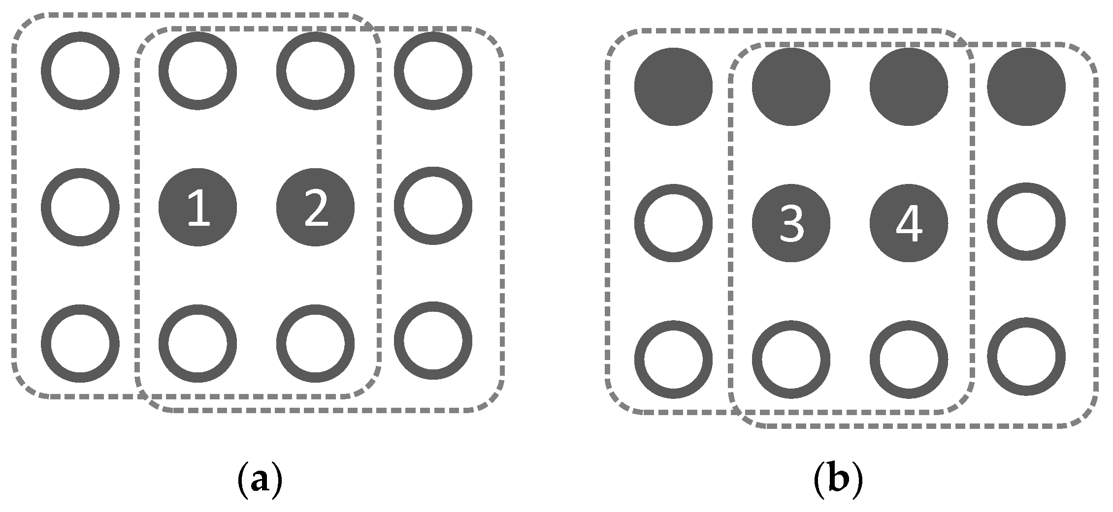
To illustrate this problem in a more straightforward manner, a schematic diagram is given as shown in Figure 2, where Figure 2a depicts the vertical gradients in the smooth image regions with the two pixels and heavily contaminated by noise, while Figure 2b shows the vertical gradients in the image edge regions without noise contamination, with the pixel gradients shown for the two pixels and . The hollow circles in the figure denote pixels of low grayscale values, while the solid circles denote pixels of high grayscale values. For convenience of discussion, it is assumed that the grayscale values of the hollow circles are 0, and the grayscale values of the solid circles are 1.
If the conventional TV regularization methods are applied to Figure 2a, pixels and are very likely to be mistaken for and preserved as image edge pixels since they have grayscale values similar to the gradients at pixels and , so that the noise cannot be effectively removed. In conventional TV models, the four pixels have an identical horizontal difference and vertical difference, so that no matter how much the threshold is, the gradients of the four pixels show consistent variation trends.
Given that the probability that a number of consecutive pixels in the smooth regions are all contaminated by noise is extremely small, this structural similarity can be used for denoising. According to (8), when K = 3 , the group gradient of pixels and is 2 , while the group gradient of pixels and is 5 . As long as the threshold is set to 2 , the noise of pixels and can be well removed, while the group gradient of pixels and shrink to 5 2 . Thus, the image edge is well preserved.
In summary, by using group gradients to calculate gradients at pixels, it is possible to highlight the difference between the highly noisy pixels in the smooth regions and the pixels in the edge regions to achieve image reconstruction in a more robust manner.

2.4. MM Algorithm

To seek the optimal solution containing the group gradient sparsity φ(V), the MM algorithm is adopted here [40]. This is a progressive method focused on finding a multivariate auxiliary function to construct an iterative series to approximate the solution for a given problem. When solving the problem of (9), the iterative cycle is expressed as (10) [34]
min v P ( V ) = { μ φ ( V ) + β 2 V V 0 2 2 }
V ( k + 1 ) = m a t { [ I + μ β D 2 ( V ( k ) ) ] 1 V 0 } , k = 1 , 2 ,
φ ( V ) (10) is defined as (7), V 0 N × N , I N 2 × N 2 denotes the identity matrix, k denotes the number of iteration steps. For any X N × N , D N 2 × N 2 is a diagonal matrix with the elements on the diagonal defined as
[ D ( X ) ] m , m = i = K l K r j = K l K r [ k 1 = K l K r k 2 = K l K r | X m i + k 1 , m j + k 2 | 2 ] 1 2
In (11), the diagonal elements of D can be calculated using MATLAB’s built-in function conv2.

3. Propose Model and Solution

In this section, a new image reconstruction model is proposed based on the Lp-quasinorm and the regularization term of group gradient sparsity as follows:
F = arg min F H F G p p + μ [ φ ( K h F ) + φ ( K v F ) ]
As mentioned above, the regularization term of the group gradient sparsity is beneficial to improving the difference between the smooth regions and the edge regions in the image after noise contamination. Meanwhile, with the ability of Lp-quasinorm in characterizing the image gradient sparsity, the proposed model is able to effectively preserve the image edge information and remove the staircase effect while blurring and denoising the image.
Next, a method for seeking a solution to the proposed model in the ADMM framework is introduced. For convenience, the following intermediate variables are introduced:
X i N × N ( i = 1 3 ) , and let { X 1 = H F G X 2 = K h F X 3 = K v F . According to the ADMM framework, an augmented Lagrangian multiplier (ALM) method [38] is adopted to solve the constrained optimization problem of (12). By doing so, the problem is transformed into an unconstrained problem whose augmented Lagrangian objective function can be expressed as
L β ( F , X 1 ~ 3 , Λ 1 ~ 3 ) = arg   min F , X 1 ~ 3 , Λ 1 ~ 3 X 1 p p + μ [ φ ( X 2 ) + φ ( X 3 ) ] β 1 Λ 1 , X 1 ( H F G ) + β 1 2 X 1 ( H F G ) 2 2 + β 1 2 Λ 1 2 β 1 2 Λ 1 2 β 2 Λ 2 , X 2 K h F + β 2 2 X 2 K h F 2 2 + β 2 2 Λ 2 2 β 2 2 Λ 2 2 β 3 Λ 3 , X 3 K v F + β 3 2 X 3 K v F 2 2 + β 3 2 Λ 3 2 β 2 2 Λ 3 2 = arg   min F , X 1 ~ 3 , Λ 1 ~ 3 X 1 p p + β 1 2 X 1 H F + G Λ 1 2 2 β 1 2 Λ 1 2 + μ φ ( X 2 ) + β 2 2 X 2 K h F Λ 2 2 2 β 2 2 Λ 2 2 + μ φ ( X 3 ) + β 3 2 X 3 K v F Λ 3 2 2 β 3 2 Λ 3 2
In (13), the dual variable Λ i N × N ( i = 1 , 2 , 3 ) is introduced as a Lagrangian multiplier, β i > 0 ( i = 1 , 2 , 3 ) is a penalty parameter which controls the linear constraint, and X , Y represents the inner product of two matrices X and Y.
It is difficult to solve the maximum value problem for the joint variable X 1 X 3 . To solve this problem, the original optimization problem is decomposed into several smaller local subproblems in the framework of ADMM [38,48], that is, X 1 X 3 are separately used in the solution-seeking process, followed by alternating iteration until the method converges to the optimal solution of the original model. The subproblems after the decomposition of (13) are as follows, where k denotes the number of iteration steps:
{ F ( k + 1 ) = arg   min F β 1 2 X 1 ( k ) H F + G Λ 1 ( k ) 2 2   + β 2 2 X 2 ( k ) K h F Λ 2 ( k ) 2 2 + β 3 2 X 3 ( k ) K v F Λ 3 ( k ) 2 2 X 1 ( k + 1 ) = arg   min X 1 X 1 p p + β 1 2 X 1 ( k ) H F ( k ) + G Λ 1 ( k ) 2 2 X 2 ( k + 1 ) = arg   min X 2 μ φ ( X 2 ) + β 2 2 X 2 ( k ) K h F ( k ) Λ 2 ( k ) 2 2 X 3 ( k + 1 ) = arg   min X 3 μ φ ( X 3 ) + β 3 2 X 3 ( k ) K v F Λ 3 ( k ) 2 2

3.1. Subproblem Solving

(1) Subproblem F
When solving subproblem F of (14), to effectively avoid the computational complexity caused by large matrix multiplication operations, a fast two-dimensional Fourier transform is introduced to transform the operation of time-domain to that of frequency-domain. The frequency domain of the subproblem F is expressed as
F ¯ ( k + 1 ) = = arg   min F β 1 2 X ¯ 1 ( k ) H ¯ F ¯ + G ¯ Λ ¯ 1 ( k ) 2 2 + β 2 2 X ¯ 2 ( k ) K ¯ h F ¯ Λ ¯ 2 ( k ) 2 2 + β 3 2 X ¯ 3 ( k ) K ¯ v F ¯ Λ ¯ 3 ( k ) 2 2
In (15), x ¯ denotes the frequency spectrum of x , and the symbol denotes element-wise matrix multiplication. Given that the right side of the formula is a smooth convex function, its first-order difference result is set to zero to find the optimal solution [5], which is obtained by using an inverse two-dimensional Fourier transform, as shown below:
F ( k + 1 ) = FFT 2 D 1 { β 1 H ¯ ( X ¯ 1 ( k ) + G ¯ Λ ¯ 1 ( k ) ) + β 2 K ¯ h ( X ¯ 2 ( k ) Λ ¯ 2 ( k ) ) + β 3 K ¯ v ( X ¯ 3 ( k ) Λ ¯ 3 ( k ) ) β 1 H ¯ H ¯ + β 2 K ¯ h K ¯ h + β 3 K ¯ v K ¯ v ) }
where F F T 2 D 1 represents the two-dimensional inverse Fourier transform, and the division symbol represents element-wise matrix division.
(2) Subproblem X 1
The subproblem X 1 of (14) is shrunk according to (17):
X 1 ( k + 1 ) = s h r i n k p ( H F ( k + 1 ) G + Λ 1 ( k ) , 1 β 1 )
where s h r i n k p ( ξ , τ ) = sgn ( ξ ) max { | ξ | τ 2 p | ξ | p 1 , 0 } is the Lp shrinkage operator, which degenerates into a soft threshold operator when p = 1.
(3) Subproblems X 2 and X 3
Subproblems X 2 and X 3 in (14) can be solved by using the following iterative loop based on the MM algorithm and (10)
X 2 ( n + 1 ) ( k + 1 ) = mat { [ I + μ β 2 D 2 ( X 2 ( n ) ( k + 1 ) ) ] 1 χ 2 ( 0 ) ( k + 1 ) } X 3 ( n + 1 ) ( k + 1 ) = mat { [ I + μ β 3 D 2 ( X 3 ( n ) ( k + 1 ) ) ] 1 χ 3 ( 0 ) ( k + 1 ) }
In (18), I N 2 × N 2 denotes the identity matrix, and X i ( n ) ( k + 1 ) ( i = 2 , 3 ) denotes the n-th iteration of the MM algorithm in the k + 1 -th outer loop.
Finally, according to the ADMM solution rule, the objective function of the dual variable Λ i ( i = 1 , 2 , 3 ) is
J 1 = m a x Λ 1 β 1 Λ 1 , ( H F ( k + 1 ) G ) X 1 ( k + 1 ) J 2 = m a x Λ 2 β 2 Λ 2 , K h F ( k + 1 ) X 2 ( k + 1 ) J 3 = m a x Λ 3 β 3 Λ 3 , K v F ( k + 1 ) X 3 ( k + 1 )
This can be updated by the ascend gradient method as (20)
Λ 1 ( k + 1 ) = Λ 1 ( k ) + γ β 1 ( H F ( k + 1 ) G X 1 ( k + 1 ) ) Λ 2 ( k + 1 ) = Λ 2 ( k ) + γ β 2 ( K h F ( k + 1 ) X 2 ( k + 1 ) ) Λ 3 ( k + 1 ) = Λ 3 ( k ) + γ β 3 ( K v F ( k + 1 ) X 3 ( k + 1 ) )
where γ is a step length parameter, also known as a relax parameter. The convergence of the ADMM algorithm has been proven when γ ( 0 , 5 + 1 2 ) [48]. The entire algorithm proposed in this study is summarized as Algorithm 1 and is named GGS_Lp.
Algorithm 1: Pseudocode GGS_Lp for image reconstruction
Input: G
Output: F
Initialize: K , k = 1 , n = 0 , X i ( k ) = 0 , Λ i ( k ) = 0 , β i ( i = 1 , 2 , 3 ) , μ , γ , p , t o l , M a x .
1: Set F ( k + 1 ) F ( k ) 2 / F ( k ) 2 as 1;
2: while F ( k + 1 ) F ( k ) 2 / F ( k ) 2 > t o l do
3:   Update F ( k + 1 ) using Equation (16);
4:   Update X 1 ( k + 1 ) using Equation (17);
5:   while n < M a x do
6:     Update X i ( n + 1 ) ( k + 1 ) ( i = 2 , 3 ) using Equation (18);
7:      X i ( k + 1 ) = X i ( n + 1 ) ( k + 1 ) ( i = 2 , 3 ) ;
8:      n = n + 1 ;
9:   end while
10:  Update Λ i ( k + 1 ) using Equation (20);
11:   k k + 1 ;
12: end while
13: Return F ( k ) as F .

3.2. Fast ADMM Solver with Restart

The convergence rate of the traditional ADMM is O ( 1 / k ) , while GGS_Lp involves calculation of the neighborhood gradient, which increases the computational burden. By introducing accelerated ADMM, the convergence rate can be increased to O ( 1 / k 2 ) [49] to improve the computational efficiency. In this section, an accelerated ADMM framework is used to solve the proposed model at a faster convergence speed. To do this, it is necessary to introduce auxiliary variables X ˜ i ( i = 1 , 2 , 3 ) and Λ ˜ i ( i = 1 , 2 , 3 ) , the acceleration step ε i ( i = 1 , 2 , 3 ) , and the sum of primal-dual residuals c i ( i = 1 , 2 , 3 ) . In the accelerated ADMM, the sum of the primal-dual residuals is monitored. With an increase in the sum, the iterative result is considered unable to converge, and thus the process is restarted to ensure high computational efficiency.
In the accelerated ADMM framework, X i   ( i = 1 , 2 , 3 ) is updated as
X 1 ( k + 1 ) = s h r i n k p ( H F ( k ) G + Λ ˜ 1 ( k ) , 1 β 1 ) X 2 ( n + 1 ) ( k + 1 ) = mat { [ I + μ β 2 D 2 ( X 2 ( n ) ( k + 1 ) ) ] 1 χ 2 ( 0 ) ( k + 1 ) } X 3 ( n + 1 ) ( k + 1 ) = mat { [ I + μ β 3 D 2 ( X 3 ( n ) ( k + 1 ) ) ] 1 χ 3 ( 0 ) ( k + 1 ) }
where X 2 ( 0 ) ( k + 1 ) = K h F ( k + 1 ) + Λ ˜ 2 ( k ) , and X 3 ( 0 ) ( k + 1 ) = K v F ( k + 1 ) + Λ ˜ 3 ( k ) .
Λ i ( i = 1 , 2 , 3 ) is updated as
Λ 1 ( k + 1 ) = Λ ˜ 1 ( k ) + γ β 1 ( H F ( k + 1 ) G X 1 ( k + 1 ) ) Λ 2 ( k + 1 ) = Λ ˜ 2 ( k ) + γ β 2 ( K h F ( k + 1 ) X 2 ( k + 1 ) ) Λ 3 ( k + 1 ) = Λ ˜ 3 ( k ) + γ β 3 ( K v F ( k + 1 ) X 3 ( k + 1 ) )
The sum of primal-dual residuals is calculated as
c i ( k + 1 ) = β 1 Λ i ( k + 1 ) Λ ˜ i ( k + 1 ) 2 2 + β Z i ( k + 1 ) Z ˜ i ( k + 1 ) 2 2 ( i = 1 , 2 , 3 )
When inequality (24) is not satisfied, the optimization process is restarted. η is a number close to 1, and is set to 0.96 to prevent the optimization process from being frequently restarted.
c i ( k + 1 ) < η c i ( k ) ( i = 1 , 2 , 3 )
When c i ( k + 1 ) < η c i ( k ) , the auxiliary variable and the acceleration step are updated as
ε i ( k + 1 ) = 1 + 1 + 4 ( ε i ( k ) ) 2 2 X ˜ i ( k + 1 ) = X i ( k + 1 ) + ε i ( k ) 1 ε i ( k + 1 ) ( X i ( k + 1 ) X i ( k ) ) , ( i = 1 , 2 , 3 ) Λ ˜ i ( k + 1 ) = Λ i ( k + 1 ) + ε i ( k ) 1 ε i ( k + 1 ) ( Λ i ( k + 1 ) Λ i ( k ) )
When a restart occurs, the variables are updated according to the following formula:
ε i ( k + 1 ) = 1 X ˜ i ( k + 1 ) = X i ( k + 1 ) Λ ˜ i ( k + 1 ) = Λ i ( k + 1 ) c i ( k + 1 ) = η 1 c i ( k ) , ( i = 1 , 2 , 3 ) .
The algorithm incorporating the accelerated ADMM is summarized as Algorithm 2 and is named GGS_LP_Fast in this study.
Algorithm 2: Pseudocode GGS_LP_Fast for image reconstruction
Input: G
Output: F
Initialize: K , k = 1 , n = 0 , X i ( k ) = 0 , Λ i ( k ) = 0 , X ˜ i ( k ) = 0 , Λ ˜ i ( k ) = 0 , ε i ( k ) = 1 , c i ( k ) = 0 , β i ( i = 1 , 2 , 3 ) , μ , γ , p , t o l , η , M a x .
1: Set F ( k + 1 ) F ( k ) 2 / F ( k ) 2 as 1;
2: while F ( k + 1 ) F ( k ) 2 / F ( k ) 2 > t o l do
3:   Update F ( k + 1 ) using Equation (16);
4:   Update X 1 ( k + 1 ) using Equation (21);
5:   while n < M a x do
6:     Update X i ( n + 1 ) ( k + 1 ) ( i = 2 , 3 ) using Equation (21);
7:      X i ( k + 1 ) = X i ( n + 1 ) ( k + 1 ) ( i = 2 , 3 ) ;
8:      n = n + 1 ;
9:   end while
10:  Update Λ i ( k + 1 ) , c i ( k + 1 ) using Equations (22) and (23);
11:  if c i ( k + 1 ) < η c i ( k ) then
12:   Update ε i ( k + 1 ) , X ˜ i ( k + 1 ) , Λ ˜ i ( k + 1 ) using Equation (25),
13:  else Update ε i ( k + 1 ) , X ˜ i ( k + 1 ) , Λ ˜ i ( k + 1 ) , c i ( k + 1 ) using Equation (26),
14:  end if
15:   k k + 1 ;
16: end while
17: Return F ( k ) as F .

4. Numerical Experiments

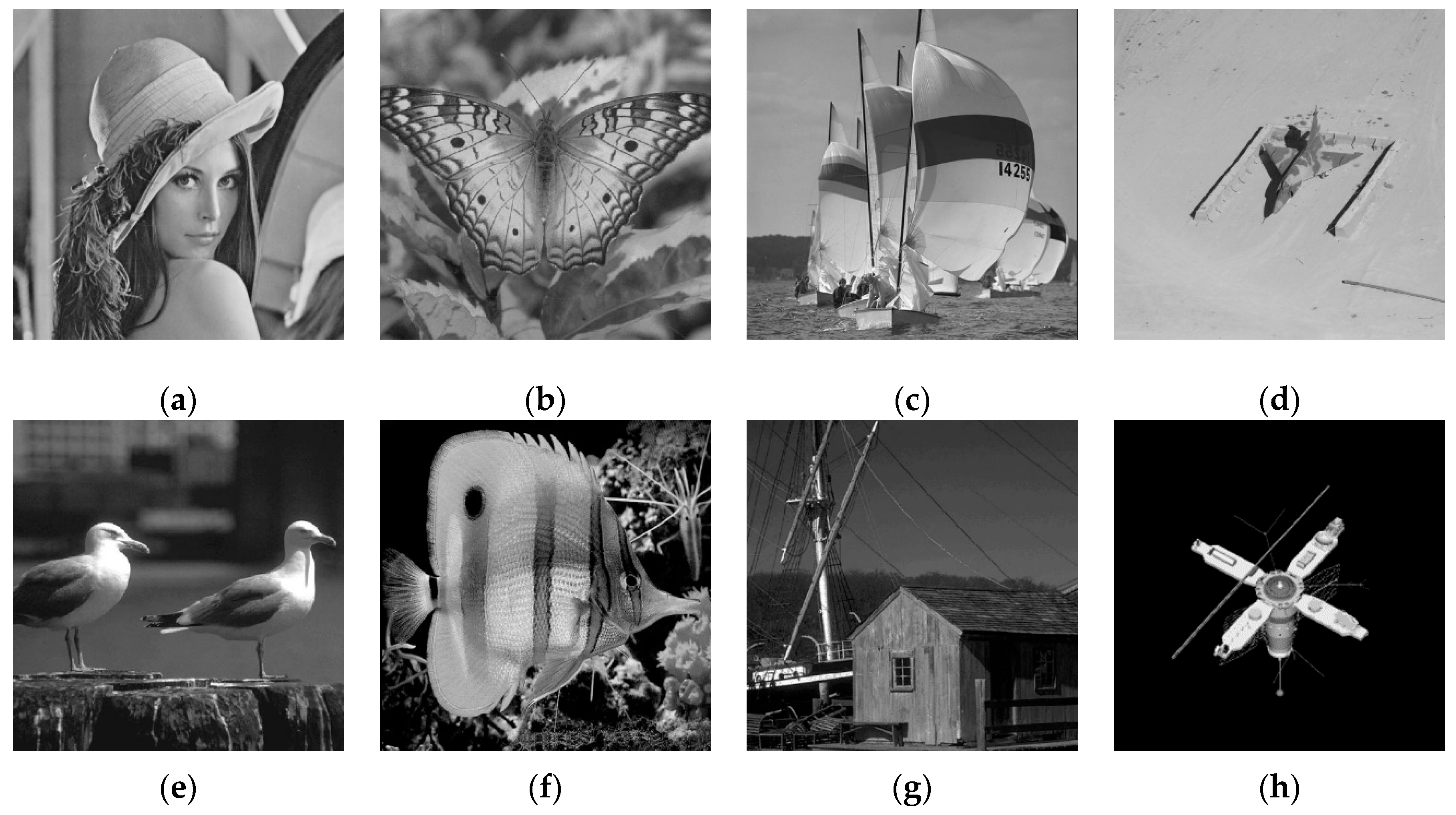
In this section, standard test images of various styles (Figure 3) are selected as experimental objects to evaluate the model proposed in this study. In particular, the image “Satellite” is downloaded from Emory University image database [50], while other images are downloaded from CVG-UGR (Computer Vision Group, University of Granada) image database [51], with each image consisting of 512 × 512 pixels. The downloaded images are converted to an image size of 256 × 256 pixels before the image reconstruction test. To verify the rationality and effectiveness of the proposed models, Gaussian blur and impulse noise are added to the experimental objects in the simulation experiment, whereby a large number of numerical experimental results are obtained to demonstrate the advantages of the proposed method.

4.1. Evaluation Criteria and Running Environment

A comparison is performed in terms of two evaluation indicators commonly used in image processing: the peak signal-to-noise ratio (PSNR) and structural similarity (SSIM) [52]. The definitions of PSNR, and SSIM are as follows:
P S N R ( X , Y ) = 10 l g 255 2 1 N 2 i = 1 N j = 1 N ( X i j Y i j ) 2
S S I M ( X , Y ) = ( 2 μ X μ Y + 255 2 k 1 2 ) ( 2 σ X Y + 255 2 k 2 2 ) ( μ X 2 + μ Y 2 + 255 2 k 1 2 ) ( σ X 2 + σ Y 2 + 255 2 k 2 2 )
In (28), X denotes the original image and Y denotes the reconstructed image; μX and μY denote the mean of X and Y, respectively; μ X 2 and μ Y 2 denote the variance of X and Y, respectively; μXY is the covariance of X and Y; and constants k1 and k2 ensure a nonzero denominator in (28), with k1 = 0.01 and k2 = 0.03 in the experiment. Generally, the larger the PSNR of the reconstructed image, the better the reconstructed image quality. The SSIM lies in the range (0, 1), and the closer the value is to 1, the higher the similarity, the better the image reconstruction effect.
In the experiment, image reconstruction effectiveness is compared between the FTVd model (The matlab code could be download from the website https://www.caam.rice.edu/~optimization/L1/ftvd/ Version 4.1.), FrTV model, TGV model, OGS_L1 model, and the two models proposed in this study (GGS_Lp and GGS_LP_Fast), both of which are frequency-domain models. To ensure the objectivity and fairness of the evaluation, the iterative conditions of the above algorithms are terminated when satisfying (29), where F ( k ) denotes the objective function of a model after the k -th iteration. In the experiment, by setting the relax parameter γ = 1.618 and adjusting the regularization parameters of each algorithm, each algorithm is allowed to operate at its best performance to ensure the objectiveness of the test results.
F ( k + 1 ) F ( k ) 2 F ( k ) 2 1 < 10 4
Hardware environment: The processor is an Intel® Core™ i7-6700 CPU @ 3.4 GHz with 16.0 GB of memory. Simulation platform: MATLAB R2018a.
Each blur kernel used in the test is generated by the built-in MATLAB function fspecial (‘gaussian’, N 1 , N 2 ), which generates a Gaussian blur kernel with a standard deviation of N 2 and window size of N 1 × N 1 , with the kernel hereinafter referred to as a G N 1 × N 1 ,   σ = N 2 kernel for simplicity. Impulse noise is added at a noise level of 30%, 40%, 50%, and 60%.

4.2. Parameter Sensitivity Analysis

4.2.1. Number of Inner Iteration Steps

When solving the X2, X3 subproblems, it is necessary to consider the number of inner iteration steps of the MM algorithm. In general, the greater the number of iteration steps, the more accurate the solution of a subproblem, but the more time-consuming the computational process. To find a proper tradeoff, the values taken by the parameter n are first explored while other parameters are fixed. Each image is subject to multiple tests at different noise levels, as exemplified below.
The images of (a) Lena, (d) plane, and (f) fish are convoluted with a G7 × 7, σ = 5 kernel at an impulse noise level of 30%. The experimental results are presented in Figure 4. As indicated by Figure 4a,b, both PSNR and SSIM are improved with an increasing number n of inner iterations, but when n exceeds 5, the promotional effect of the iteration step number on PSNR and SSIM becomes less significant. With an increase in the iteration step number, the computational time increases, Figure 4c. As shown in Figure 4a,b, some of the values have little dropped as the graph is progressed, which is because the other parameters do not be tuned to the best for different n. Based on a comprehensive consideration of the computational time and optimal PSNR and SSIM values, the number of inner iteration steps is set to 5 in the subsequent test.

4.2.2. Group Gradient Parameter K

The group gradient parameter K of the proposed algorithm is tested and compared to evaluate its effect on the overall performance of the algorithms. Given a different image and a different noise level, K is continuously changed from 1 to 10, and at each value, multiple tests are performed. Take the image of (e) seabird as an example, which is convoluted with a G 7 × 7 ,   σ = 5 blur kernel at noise levels of 30%, 40%, 50%, and 60%. The PSNR and SSIM results are recorded under these different scenarios, as shown in Figure 5. When K = 1 , the algorithm degenerates into a traditional ATV model.
As shown in Figure 5, an increase in K has different effects on PSNR and SSIM at different noise levels. For example, at a 30% noise level with K = 5 , both PSNR and SSIM reach their maximum values, and this trend is invariant. It is evident that given a low noise level, the neighborhood information of the image has positive effects on the algorithm performance. However, when the noise level is 60%, the structural characteristics of the neighborhood gradient are seriously damaged, and in this circumstance, a greater K may lead to decreased algorithm performance.
In addition, the greater the parameter K , the more information is used from the neighborhood during the computation and the higher the computational complexity, thus increasing the computational time. With K set to a proper value, the proposed algorithm has a greater capability to preserve image edges and to resist high-level noise. Based on a comprehensive consideration of both computational time and the optimal PSNR and SSIM values, K is set to 3 in the subsequent test.

4.2.3. Regularization Parameter μ and Quasinorm p

Next, the effects of regularization parameter μ on the test results are evaluated. Given a different test image at various impulse noise levels, μ is gradually increased from a small value to a high value while the values of PSNR and SSIM of image reconstruction are recorded. Here, take the test images of (c) boat and (g) house as examples, where the images are convoluted with a G 7 × 7 , σ = 5 blur kernel at noise levels of 30%, 40%, 50%, and 60%, respectively, while the values of PSNR at various values of μ are recorded, as shown in Figure 6. The experimental results show that given a test image, PSNR is relatively stable when μ is greater than a certain value, suggesting that the proposed algorithm is not sensitive to the regularization parameter μ . That is, the optimal values of μ are relatively stable, and the proposed algorithm is robust. In the subsequent experiment, μ is set to 100, 90, 80, and 60 at noise levels of 30%, 40%, 50%, and 60%, respectively.
With the above-determined parameters, p is allowed to vary from 0 to 1 in steps of 0.05 in light of the characteristics of the impulse noise, and a loop statement is used for a thorough search for the p value that optimizes PSNR, as shown in Table 1. Test images are convoluted with a G 7 × 7 ,   σ = 5 blur kernel at noise levels of 30%, 40%, 50%, and 60%, respectively. The results show that to a certain test image, the p value that optimizes PSNR is relatively stable.

4.2.4. Comparative Testing of Image Reconstruction Effectiveness between Several Algorithms

To further test the effectiveness of the proposed algorithm, tests are subject to in-depth comparisons with other state-of-the-art algorithms. The group of images in Figure 3 is used as the test objects, which are convoluted with a G 7 × 7 ,   σ = 5 blur kernel at impulse noise levels of 30%, 40%, 50%, and 60%, respectively. The test results for the different images are listed in Table 2, with the optimal indicators highlighted in boldface and black font.
Based on the data in the above table, the following conclusions can be drawn:
  • With the addition of blurring and different levels of noise in various images, the proposed models in this study are superior to other excellent models for image reconstruction in terms of PSNR and SSIM. This indicates that the proposed models have good deblurring and denoising performance, while allowing the reconstructed images to be more similar to the original images.
  • When the proposed models are employed to reconstruct the eight images, the PSNR values are higher than those of the TGV model by 0.204–2.177 dB, and the superiority of the proposed models is more evident at higher levels of noise. For example, PSNR of the proposed models (28.081 dB) is 2.177 dB higher than that of the TGV model (25.904 dB) for the image of Lena at a noise level of 60%, and the PSNR difference becomes 2.174 dB for the image of the boat at the same noise level (26.797 dB vs. 24.623 dB).
  • Compared with OGS_L1, the proposed models increase the Lp-quasinorm shrinkage and improve the ability to characterize image gradient sparsity. When recovering the eight images, the proposed models have PSNR values that are 0.328–1.964 dB higher than those of the OGS_L1 model. For the butterfly image at the noise level of 60%, PSNR of the proposed models (26.077 dB) is 1.964 dB higher than that of the OGS_L1 model (24.113 dB).
To better understand the test results, some reconstructed images are illustrated below:
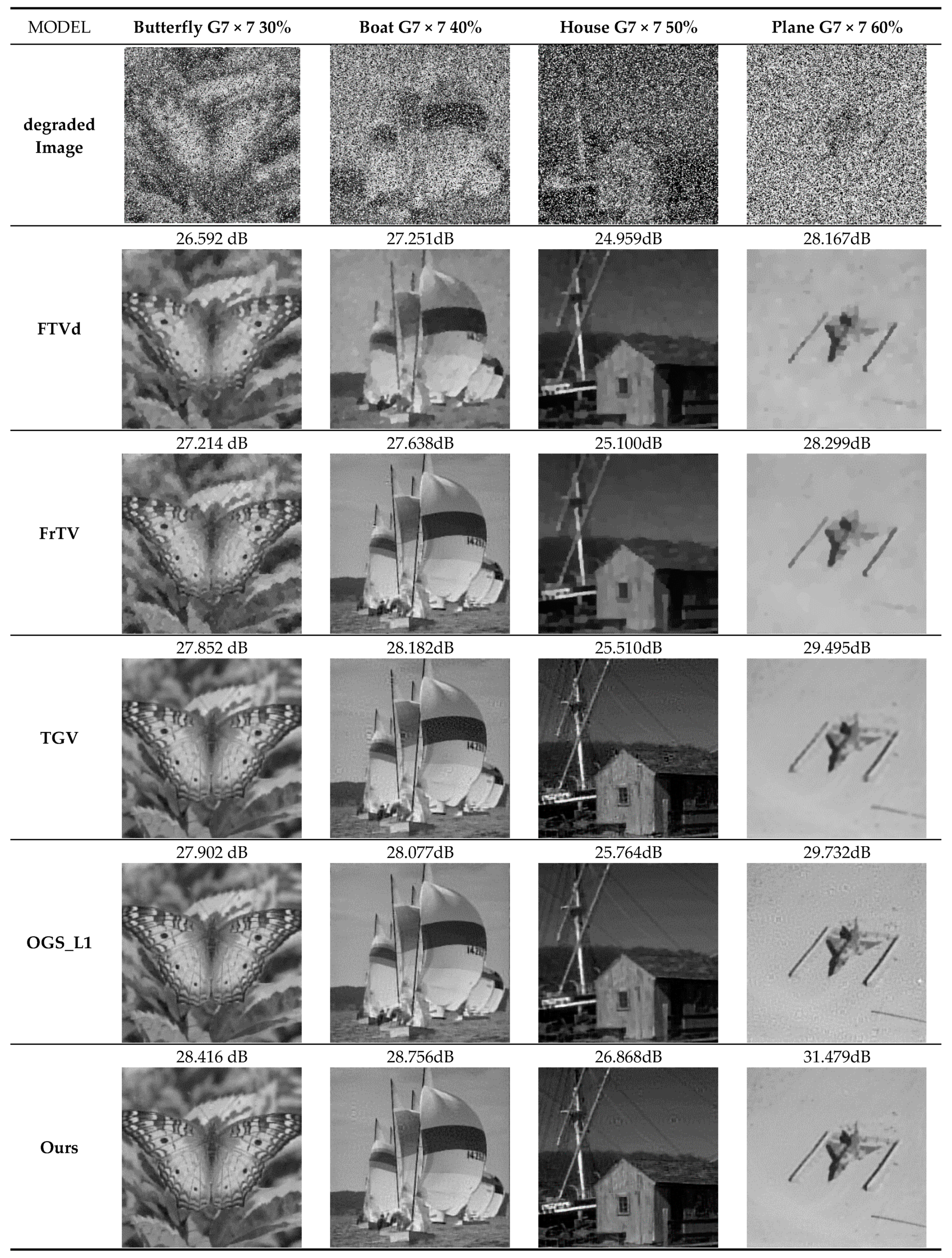
Figure 7 depicts the image reconstruction results of several models for the butterfly, boat, house, and plane images blurred by convolution with a G 7 × 7 ,   σ = 5 blur kernel at impulse noise levels of 30–60%. The proposed model of this study shows good image reconstruction performance at each noise level, with PSNR values greater than those of the other advanced models. It is noteworthy that even in the presence of high-level noise contamination, the proposed algorithm is still able to provide the reconstructed images with good visual effect.
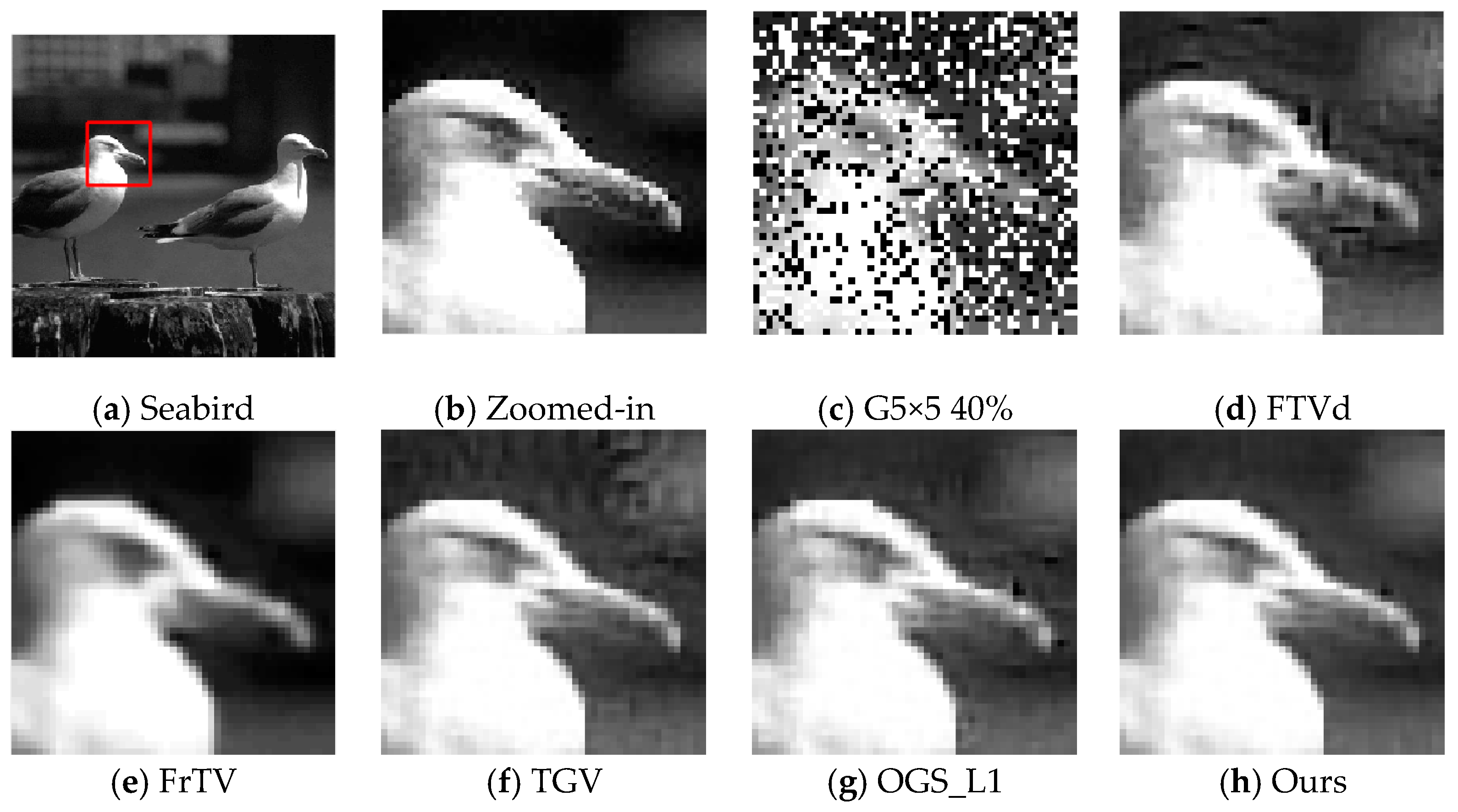
Figure 8 depicts zoomed-in seabird images recovered by several models after image blurring owing to a G 5 × 5 ,   σ = 5 blur kernel at a 40% level of impulse noise. As shown by the visual effects of the image recovery results, the FTVd method leads to a staircase effect in the recovered image, as shown in Figure 8d. The protectory effect of the FrTV method on the image edges needs to be improved, as shown in Figure 8e. The TGV and OGS_L1 methods have satisfactory inhibitory performance on the staircase effect, but local areas of the TGV-reconstructed image still contain some highly noisy pixels, as shown in Figure 8f,g. The OGS_L1 method reconstruction leads to relatively smooth image reconstruction results for smooth image regions, but some image edges are oversmoothed. The proposed model is able to reconstruct the image pixels of similar grayscale values in the smooth image regions well, and avoids the staircase effect while preserving the image edges, thereby providing a satisfactory overall reconstruction performance.
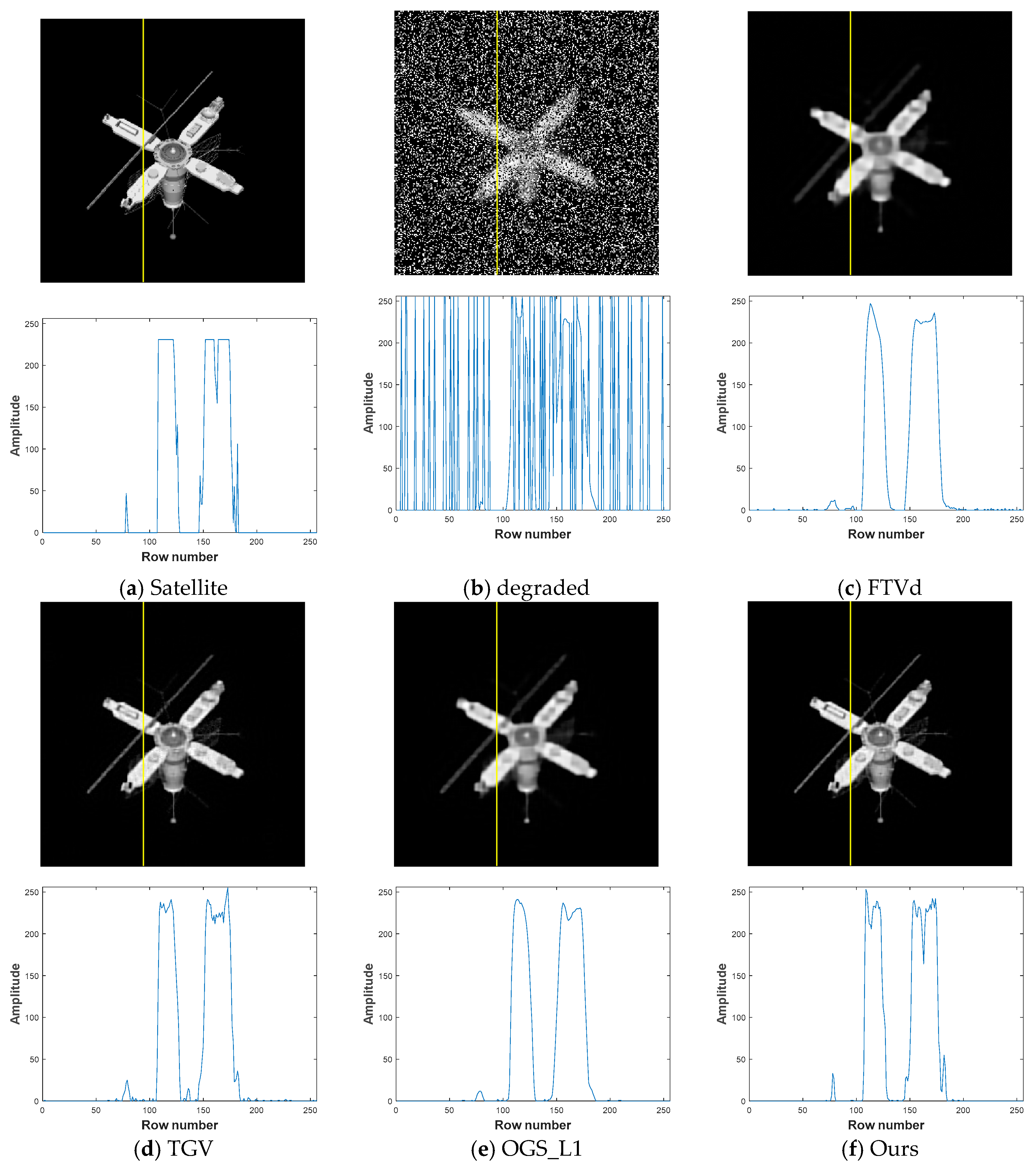
Figure 9 depicts a comparison of grayscale values in single channels of the satellite image as recovered by several algorithms after image blurring with a G 9 × 9 ,   σ = 5 blur kernel at an impulse noise level of 40%. To further compare the results of various models, the 100th-channel signals are extracted from the image. It is evident that the TGV-reconstructed image still contains some noise-contaminated pixels in some local areas, as shown in Figure 9d. In Figure 9e, the OGS_L1 algorithm results in thorough noise removal, but the image edges are oversmoothed to some extent. The proposed algorithm can remove the noise entirely while preserving the image edges well, as shown in Figure 9f.

4.2.5. Comparison of Image Reconstruction Time for Several Algorithms

Finally, to further test the timeliness of the proposed models, the mean time spent for image reconstruction is compared between the FTVd, TGV, and OGS_L1 models and the proposed models under the premise that the abovementioned test procedures are free of bias. Here, the proposed models in this study are named the GGS_Lp model and the GGS_LP_Fast model, with the latter being a model for accelerated restart of the former. In the test, images are blurred with a G 7 × 7 ,   σ = 5 blur kernel at impulse noise levels of 30–60%. The test results are partially presented in Table 3, with the optimal results highlighted in boldface and black font.
Analysis of the data in Table 3 leads to the following conclusions:
  • The GGS_Lp model and its accelerated restart version GGS_LP_Fast, both proposed in this study, lead to similar PSNR values when the two models are used to reconstruct images, but their PSNR values are all greater than those of the FTVd, TGV, and OGS_L1 models.
  • As a classic algorithm, FTVd is still advantageous in terms of computational speed. TGV and OGS_L1 give better image reconstruction results than FTVd, but they are more time-consuming. In this study, neighborhood gradient information is thoroughly considered, and the Lp-quasinorm is introduced as a regularization constraint, which leads to a greater computational complexity and thereby greater time consumption for image reconstruction compared with the FTVd model. By contrast, the GGS_LP_Fast model increases computational efficiency to a great extent, and its performance is especially prominent for images with a high level of noise.

5. Conclusions

This study proposed a new image reconstruction method based on total variation regularization incorporating Lp-quasinorm and group gradient sparsity to deblur images and remove impulse noise. This method, in which the regularization term of the group gradient sparsity can retrieve the neighborhood information of an image gradient, and in which the Lp-quasinorm constraint can characterize the gradient sparsity, can effectively deblur and denoise images to reduce the staircase effect and well preserve the image edges. A large number of numerical experiments showed that the proposed method has good overall performance for image reconstruction. The number of inner iteration steps of the MM algorithm and the group gradient parameter K can be set based on a comprehensive consideration of both computational time and the optimal PSNR and SSIM values. Regularization parameter μ and quasinorm p values are relatively stable, which shows that the proposed algorithm is robust. It is noteworthy that the proposed model uses a generalized regularization term applicable to other image reconstruction problems. Thus, the model has wide applicability.

Author Contributions

Funding acquisition, F.Y. Methodology, F.L., Y.C. (Yingpin Chen) and L.W. Software, F.L., Y.C. (Yingpin Chen) and W.Z.; Writing—Original draft, F.L.; Writing-review and editing, F.L., Y.C. (Yuqun Chen) and Y.C. (Yingpin Chen).

Funding

This work is supported by the Foundation of Fujian Province Great Teaching Reform [FBJG20180015], the Education and Scientific Research Foundation of Education Department of Fujian Province for Young and Middle-aged Teachers [grant number JT180310, JT180309, JT180311, JAT170352] and the Open Foundation of Digital Signal and Image Processing Key Laboratory of Guangdong Province [grant number 2017GDDSIPL-01]. Natural Science Foundation of Fujian Province [2017J01708].

Acknowledgments

The authors appreciate Professor Tingzhu Huang and Doctor Gang Liu of the University of Electronic Science and Technology of China for sharing the OGS_L1 code.

Conflicts of Interest

The authors declare no conflict of interest.

References

  1. Gonzalez, R.C. Digital Image Processing; Prentice Hall: Upper Saddle River, NJ, USA, 2016. [Google Scholar]
  2. Karayiannis, N.B.; Venetsanopoulos, A.N. Regularization theory in image restoration—The stabilizing functional approach. IEEE Trans. Acoust. Speech Signal Process. 1990, 38, 1155–1179. [Google Scholar] [CrossRef]
  3. Tikhonov, A.N.; Goncharsky, A.V.; Stepanov, V.V.; Yagola, A.G. Numerical Methods for the Solution of Ill-Posed Problems; Springer Science & Business Media: Berlin, Germany, 1995. [Google Scholar]
  4. Chen, Y.; Peng, Z.; Gholami, A.; Yan, J. Seismic signal sparse time-frequency analysis by Lp-quasinorm constraint. arXiv, 2018; arXiv:1801.05082. [Google Scholar]
  5. Lin, F.; Yu, F.; Chen, Y.; Li, M.; Peng, Z. Seismic signal denoising using total generalized variation with overlapping group sparsity in the accelerated ADMM framework. J. Geophys. Eng. 2019. [Google Scholar] [CrossRef]
  6. Mousavi Kahaki, S.M.; Nordin, M.J.; Ashtari, A.H.; Zahra, S.J. Invariant Feature Matching for Image Registration Application Based on New Dissimilarity of Spatial Features. PLoS ONE 2016, 11, e0149710. [Google Scholar] [CrossRef] [PubMed]
  7. Kahaki, S.M.M.; Nordin, M.J.; Ashtari, A.H.; Zahra, S.J. Deformation invariant image matching based on dissimilarity of spatial features. Neurocomputing 2016, 175, 1009–1018. [Google Scholar] [CrossRef]
  8. Phillips, D.L. A Technique for the Numerical Solution of Certain Integral Equations of the First Kind. J. ACM 1962, 9, 84–97. [Google Scholar] [CrossRef]
  9. Tihonov, A.N. Solution of incorrectly formulated problems and the regularization method. Sov. Math. 1963, 4, 1035–1038. [Google Scholar]
  10. Rudin, L.I.; Osher, S.; Fatemi, E. Nonlinear total variation based noise removal algorithms. Phys. D Nonlinear Phenom. 1992, 60, 259–268. [Google Scholar] [CrossRef]
  11. Lassen, A.L. Implementation and Evaluation of a Splitting Method for Total Variation Deblurring; Technical University of Denmark: Lyngby, Denmark, 2011. [Google Scholar]
  12. Guo, X.; Li, F.; Ng, M.K. A fast ℓ 1-TV algorithm for image restoration. SIAM J. Sci. Comput. 2009, 31, 2322–2341. [Google Scholar] [CrossRef]
  13. Chambolle, A. An algorithm for total variation minimization and applications. J. Math. Imaging Vis. 2004, 20, 89–97. [Google Scholar]
  14. Salvadeo, D.H.P.; Mascarenhas, N.D.A.; Levada, A.L.M. Nonlocal Markovian models for image denoising. J. Electron. Imaging 2016, 25, 013003. [Google Scholar] [CrossRef]
  15. Chan, T.; Esedoglu, S.; Park, F.; Yip, A. Recent developments in total variation image restoration. Math. Models Comput. Vis. 2005, 17, 1–18. [Google Scholar]
  16. Yang, J.; Zhang, Y.; Yin, W. An efficient TVL1 algorithm for deblurring multichannel images corrupted by impulsive noise. SIAM J. Sci. Comput. 2009, 31, 2842–2865. [Google Scholar] [CrossRef]
  17. Huang, G.; Jiang, H.; Matthews, K.; Wilford, P. Lensless Imaging by Compressive Sensing. In Proceedings of the IEEE International Conference on Image Processing, Melbourne, Australia, 15–18 September 2013; pp. 2101–2105. [Google Scholar]
  18. Chen, Y.; Peng, Z.; Cheng, Z.; Tian, L. Seismic signal time-frequency analysis based on multi-directional window using greedy strategy. J. Appl. Geophys. 2017, 143, 116–128. [Google Scholar] [CrossRef]
  19. Lu, T.; Li, S.; Fang, L.; Ma, Y.; Benediktsson, J.A. Spectral–spatial adaptive sparse representation for hyperspectral image denoising. IEEE Trans. Geosci. Remote Sens. 2016, 54, 373–385. [Google Scholar] [CrossRef]
  20. Zhao, W.; Lu, H. Medical Image Fusion and Denoising with Alternating Sequential Filter and Adaptive Fractional Order Total Variation. IEEE Trans. Instrum. Meas. 2017, 66, 2283–2294. [Google Scholar] [CrossRef]
  21. Wu, L.; Chen, Y.; Jin, J.; Du, H.; Qiu, B. Four-directional fractional-order total variation regularization for image denoising. J. Electron. Imaging 2017, 26, 053003. [Google Scholar] [CrossRef]
  22. Bredies, K. Symmetric tensor fields of bounded deformation. Annali di Matematica Pura ed Applicata 2013, 192, 815–851. [Google Scholar] [CrossRef]
  23. Bredies, K.; Holler, M. Regularization of linear inverse problems with total generalized variation. J. Inverse Ill-Posed Probl. 2014, 22, 871–913. [Google Scholar] [CrossRef]
  24. Bredies, K.; Kunisch, K.; Pock, T. Total generalized variation. SIAM J. Imaging Sci. 2010, 3, 492–526. [Google Scholar] [CrossRef]
  25. Knoll, F.; Bredies, K.; Pock, T.; Stollberger, R. Second order total generalized variation (TGV) for MRI. Magn. Reson. Med. 2011, 65, 480–491. [Google Scholar] [CrossRef]
  26. Kong, D.; Peng, Z. Seismic random noise attenuation using shearlet and total generalized variation. J. Geophys. Eng. 2015, 12, 1024–1035. [Google Scholar] [CrossRef]
  27. Zhang, X.; Burger, M.; Bresson, X.; Osher, S. Bregmanized nonlocal regularization for deconvolution and sparse reconstruction. SIAM J. Imaging Sci. 2010, 3, 253–276. [Google Scholar] [CrossRef]
  28. Zhang, X.; Chan, T.F. Wavelet inpainting by nonlocal total variation. Inverse Probl. Imaging 2017, 4, 191–210. [Google Scholar]
  29. Ren, Z.; He, C.; Zhang, Q. Fractional order total variation regularization for image super-resolution. Signal Process. 2013, 93, 2408–2421. [Google Scholar] [CrossRef]
  30. Wang, Y.; Yang, J.; Yin, W.; Zhang, Y. A new alternating minimization algorithm for total variation image reconstruction. SIAM J. Imaging Sci. 2008, 1, 248–272. [Google Scholar] [CrossRef]
  31. Sakurai, M.; Kiriyama, S.; Goto, T.; Hirano, S. Fast algorithm for total variation minimization. In Proceedings of the 2011 18th IEEE International Conference on Image Processing (ICIP), Brussels, Belgium, 11–14 September 2011; pp. 1461–1464. [Google Scholar]
  32. Selesnick, I.; Farshchian, M. Sparse signal approximation via nonseparable regularization. IEEE Trans. Signal Process. 2017, 65, 2561–2575. [Google Scholar] [CrossRef]
  33. Selesnick, I.W.; Chen, P.-Y. Total variation denoising with overlapping group sparsity. In Proceedings of the Acoustics, Speech and Signal Processing (ICASSP), Vancouver, BC, Canada, 26–31 May 2013; pp. 5696–5700. [Google Scholar]
  34. Liu, G.; Huang, T.Z.; Liu, J.; Lv, X.-G. Total variation with overlapping group sparsity for image deblurring under impulse noise. PLoS ONE 2015, 10, e0122562. [Google Scholar] [CrossRef]
  35. Liu, J.; Huang, T.Z.; Liu, G.; Wang, S.; Lv, X.G. Total variation with overlapping group sparsity for speckle noise reduction. Neurocomputing 2016, 216, 502–513. [Google Scholar] [CrossRef]
  36. Donoho, D.L.; Elad, M. Optimally sparse representation in general (nonorthogonal) dictionaries via ℓ1 minimization. Pro. Natl. Acad. Sci. USA 2003, 100, 2197–2202. [Google Scholar] [CrossRef]
  37. Woodworth, J.; Chartrand, R. Compressed sensing recovery via nonconvex shrinkage penalties. Inverse Probl. 2016, 32, 75004–75028. [Google Scholar] [CrossRef]
  38. Nocedal, J.; Wright, S.J. Numerical Optimization; Springer: New York, NY, USA, 2006; pp. 29–76. [Google Scholar]
  39. De Vieilleville, F.; Weiss, P.; Lobjois, V.; Kouame, D. Alternating direction method of multipliers applied to 3D light sheet fluorescence microscopy image deblurring using GPU hardware. In Proceedings of the International Conference of the IEEE Engineering in Medicine & Biology Society, Boston, MA, USA, 30 August–3 September 2011; p. 4872. [Google Scholar]
  40. Chen, P.Y.; Selesnick, I.W. Translation-invariant shrinkage/thresholding of group sparse signals. Signal Process. 2014, 94, 476–489. [Google Scholar] [CrossRef] [Green Version]
  41. Kahaki, S.M.M.; Arshad, H.; Nordin, M.J.; Ismail, W. Geometric feature descriptor and dissimilarity-based registration of remotely sensed imagery. PLoS ONE 2018, 13, e0200676. [Google Scholar] [CrossRef] [PubMed]
  42. Eybposh, M.H.; Turani, Z.; Mehregan, D.; Nasiriavanaki, M. Cluster-based filtering framework for speckle reduction in OCT images. Biomed. Opt. Express 2018, 9, 6359–6373. [Google Scholar] [CrossRef]
  43. Adabi, S.; Rashedi, E.; Clayton, A.; Mohebbi-Kalkhoran, H.; Chen, X.W.; Conforto, S.; Nasiriavanaki, M. Learnable despeckling framework for optical coherence tomography images. J. Biomed. Opt. 2018, 23, 016013. [Google Scholar] [CrossRef] [PubMed] [Green Version]
  44. Nikolova, M. A variational approach to remove outliers and impulse noise. J. Math. Imaging Vis. 2004, 20, 99–120. [Google Scholar] [CrossRef]
  45. Zheng, L.; Maleki, A.; Weng, H.; Wang, X.; Long, T. Does ℓp-minimization outperform ℓ1-minimization? IEEE Trans. Inf. Theory 2017, 63, 6896–6935. [Google Scholar] [CrossRef]
  46. Liu, C.; Shi, Z.; Hou, T.Y. On the Uniqueness of Sparse Time-Frequency Representation of Multiscale Data. Multiscale Model. Simul. 2015, 13, 790–811. [Google Scholar] [CrossRef] [Green Version]
  47. Liu, J.; Huang, T.Z.; Selesnick, I.W.; Lv, X.G.; Chen, P.Y. Image restoration using total variation with overlapping group sparsity. Inf. Sci. 2015, 295, 232–246. [Google Scholar] [CrossRef]
  48. Boyd, S.; Parikh, N.; Chu, E.; Peleato, B.; Eckstein, J. Distributed optimization and statistical learning via the alternating direction method of multipliers. Found. Trends® Mach. Learn. 2011, 3, 1–122. [Google Scholar] [CrossRef]
  49. Goldstein, T.; O’Donoghue, B.; Setzer, S.; Baraniuk, R. Fast alternating direction optimization methods. SIAM J. Imaging Sci. 2014, 7, 1588–1623. [Google Scholar] [CrossRef]
  50. Emory University Image Database. Available online: http://www.mathcs.emory.edu/~nagy/RestoreTools/ (accessed on 15 March 2018).
  51. CVG-UGR (Computer Vision Group, University of Granada) Image Database. Available online: http://decsai.ugr.es/cvg/dbimagenes/index.php (accessed on 15 March 2018).
  52. Wang, Z.; Bovik, A.C.; Sheikh, H.R.; Simoncelli, E.P. Image quality assessment: From error visibility to structural similarity. IEEE Trans. Image Process. 2004, 13, 600–612. [Google Scholar] [CrossRef]
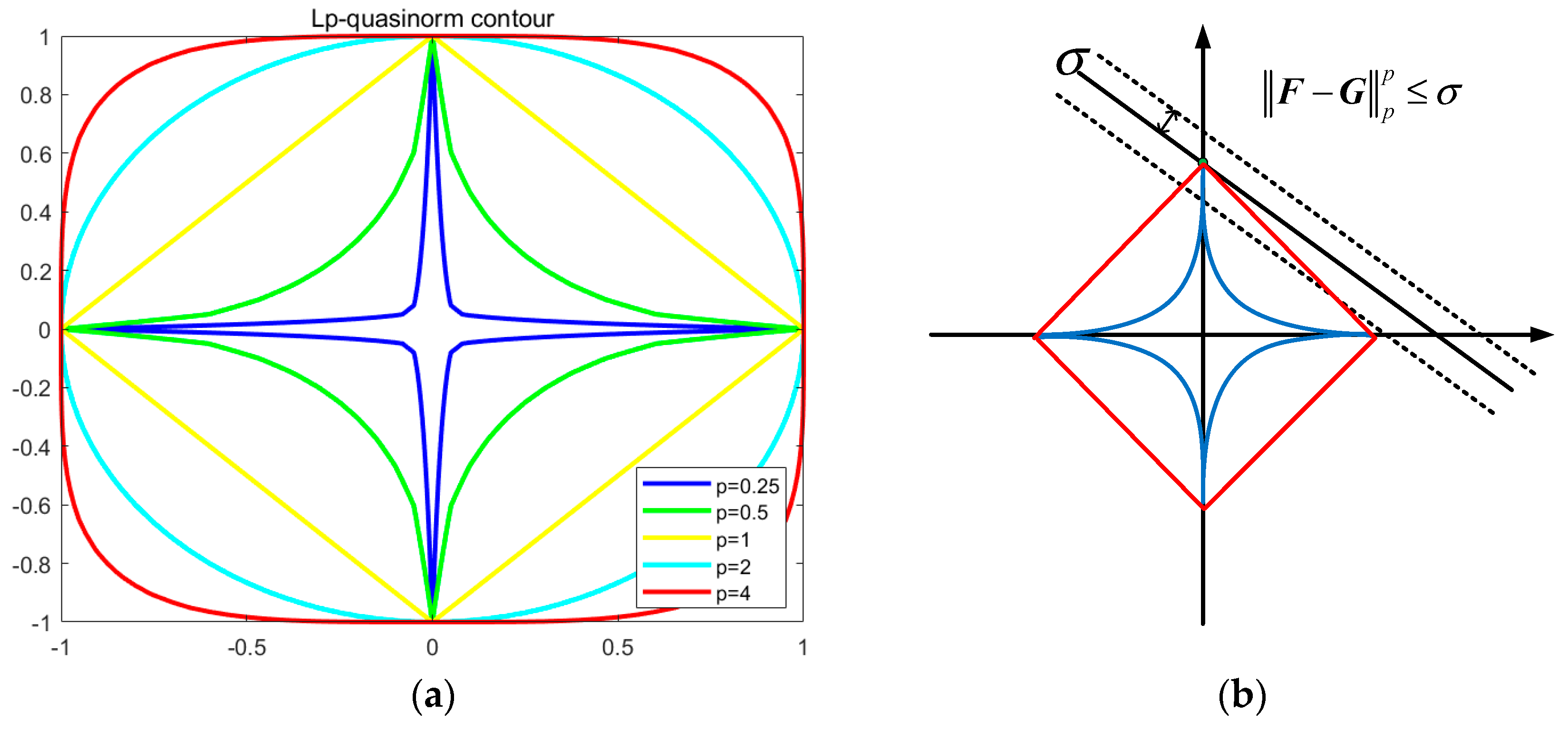
Figure 1. Schematic diagram of feasible domains for various norms. (a) Lp-quasinorm contour: p takes values of 0.25, 0.5, 1, 2, and 4 from inner to outer contour lines; (b) Feasible domains for 0 < p < 1 (blue) and p = 1 (red).
Information 10 00115 g001
Figure 2. Two-dimensional diagram of sparse groups: (a) smooth region contaminated by noise and (b) edge region not contaminated by noise.
Information 10 00115 g002
Figure 3. Test images: (a) Lena, (b) butterfly, (c) boat, (d) plane, (e) seabird, (f) fish, (g) house, and (h) satellite.
Information 10 00115 g003
Figure 4. Effects of iteration steps number on the results: (a) PSNR, (b) SSIM, and (c) processing time.
Information 10 00115 g004
Figure 5. Effects of group gradient parameter K on experimental results: (a) PSNR, (b) SSIM, and (c) processing time.
Information 10 00115 g005
Figure 6. Effects of regularization parameter μ on experimental results (a–d) refer to effect of μ on PSNR at noise levels of 30%, 40%, 50%, and 60%, respectively.
Information 10 00115 g006
Figure 7. Random examples of images reconstructed by several advanced models and proposed model. Top row depicts the blurred and noisy images of the butterfly, boat, house, and plane owing to convolution with a G 7 × 7 ,   σ = 5 blur kernel and impulse noise levels of 30%, 40%, 50%, and 60%.
Information 10 00115 g007
Figure 8. Comparison of the zoomed-in views of reconstructed images by several advanced models and proposed model: (a) selected area, (b) zoomed-in part of selected area, (c) blurred and noisy zoomed-in part owing to convolution with a G 5 × 5 ,   σ = 5 blur kernel at a impulse noise level of 40%, and (dh) zoomed-in parts of reconstructed images by FTVd, FrTV, TGV, OGS_L1, and proposed model, respectively.
Information 10 00115 g008
Figure 9. Comparison of the proposed model and several advanced models in terms of the 100th-channel data of the reconstructed satellite images. (a) refers to the grayscale values of the 100th pixel channel in the original satellite image, with the yellow vertical line on the figure indicating the 100th-channel position. (b) refers to a blurred image owing to convolution with a G 9 × 9 ,   σ = 5 blur kernel at impulse noise level of 40%. (cf) depict images with grayscale values of the 100th channel recovered by the FTVd, TGV, OGS_L1, and proposed algorithms, respectively.
Information 10 00115 g009
Table 1. The p value that optimizes PSNR for different images.
Noise LevelLenaButterflyBoatPlaneSeabirdFishHouseSatellite
300.650.450.550.550.500.650.700.75
400.650.450.550.550.500.650.700.75
500.650.450.550.550.500.650.700.75
600.650.500.550.550.500.650.700.75
Table 2. PSNR (dB) and SSIM values generated by various algorithms in deblurring and denoising different images.
ImagesNoise LevelFTVdFrTVTGVOGS_L1Ours
PSNRSSIMPSNRSSIMPSNRSSIMPSNRSSIMPSNRSSIM
Lena3027.1210.81328.7420.85429.1080.86329.4430.87529.8250.889
4025.2700.75026.3410.77328.5890.84228.7500.85729.5510.878
5023.8430.65424.5080.76027.6730.81027.8990.83228.8990.859
6021.8610.59222.8230.61125.9040.67226.4440.79428.0810.831
Butterfly3026.5920.81327.2140.82427.8520.85427.9020.85928.4160.875
4026.0130.78226.3780.80327.0780.82926.9960.82727.7320.837
5025.4330.76126.0150.79126.4290.79426.5270.77026.9170.817
6024.7310.73024.9090.74125.0410.75224.1130.72126.0770.771
Boat3027.5430.86028.0400.86529.0280.88128.9380.88029.2660.883
4027.2510.85127.6380.86228.1820.86328.0770.86128.7560.868
5025.7030.82026.3250.82626.7330.84226.5940.82727.9970.860
6023.9020.73124.2330.76024.6230.78124.9230.78226.7970.828
Plane3030.2450.77230.5510.83331.6490.89132.7510.90733.2810.913
4029.8690.87230.5380.85131.3620.88332.0920.89132.8370.919
5029.0720.85129.5560.86231.1260.88131.3710.88332.1210.890
6028.1670.80328.2990.84129.4950.71229.7320.87731.4790.885
Seabird3029.3770.87229.7500.88231.3440.89131.8430.91032.2140.913
4028.5000.86328.9510.86830.5300.88030.8110.88931.7000.908
5027.6360.82928.0730.84429.1560.85529.4180.86430.2490.875
6026.5940.81227.0100.80327.8810.85227.9380.84029.2150.853
Fish3023.1110.69323.7520.73024.5540.77224.3500.76424.7580.788
4022.8500.66123.0320.70023.3100.68223.5470.73724.1500.755
5021.8960.62322.6490.68122.8810.69222.5720.68523.5850.726
6020.9330.57221.0510.58121.1130.58321.1090.60122.4580.675
House3026.5580.77126.7910.77328.3220.83228.2830.83328.6590.847
4026.1510.75026.5730.76027.9720.82127.5010.80628.2460.822
5024.9590.69325.1000.70125.5100.72225.7640.72426.8680.778
6024.1100.67024.2120.67424.7270.68424.3150.67325.6920.726
Satellite3028.3720.93429.1900.94230.9300.96331.7510.96732.7320.977
4028.0740.93128.6350.91130.7450.95230.2960.96232.3620.974
5027.4030.92127.6820.92329.8740.95130.0950.95131.3970.954
6026.2450.90126.4530.90928.1520.93128.2890.94229.8450.949
Table 3. Mean time (S) spent by several algorithms in deblurring different images.
ImagesNoise LevelFTVdTGVOGS_L1GGS_LPGGS_LP_Fast
PSNRTimePSNRTimePSNRTimePSNRTimePSNRTime
Lena3027.1211.0229.1085.1229.4431.7229.8252.5629.9201.14
6021.8611.9825.9048.3426.4443.1028.0813.4527.9132.10
Butterfly3026.5921.3327.8526.0127.9020.9628.4162.0628.5731.25
6024.7311.8825.0419.2624.1132.8226.0772.9525.8271.83
Boat3027.5430.8329.0284.9828.9382.2529.2661.4829.5861.61
6023.9021.9524.6239.3024.9232.4626.7973.0426.6882.17
Plane3030.2450.7231.6493.4732.7511.2533.2812.2832.9091.59
6028.1671.8429.4955.9229.7323.9331.4794.0931.3872.82
Seabird3029.3771.5631.3445.6431.8432.4032.2141.7032.5281.87
6026.5942.3527.8819.7627.9383.7329.2153.8429.1832.29
Fish3023.1110.9224.5546.2324.3501.5324.7581.3624.8331.17
6020.9331.9021.11310.8521.1093.0722.4582.5922.3861.87
House3026.5581.1528.3226.2428.2831.3628.6591.5928.8841.62
6024.1102.3824.72711.2324.3152.3725.6923.3425.5852.29
Satellite3028.3720.7630.9303.6931.7511.3932.7321.6732.7991.14
6026.2451.8828.1527.8628.2892.8529.8451.7030.0131.60