Abstract
Traffic prediction techniques are classified as having parametric, non-parametric, and a combination of parametric and non-parametric characteristics. The extreme learning machine (ELM) is a non-parametric technique that is commonly used to enhance traffic prediction problems. In this study, a modified probability approach, continuous conditional random fields (CCRF), is proposed and implemented with the ELM and then utilized to assess highway traffic data. The modification is conducted to improve the performance of non-parametric techniques, in this case, the ELM method. This proposed method is then called the distance-to-mean continuous conditional random fields (DM-CCRF). The experimental results show that the proposed technique suppresses the prediction error of the prediction model compared to the standard CCRF. The comparison between ELM as a baseline regressor, the standard CCRF, and the modified CCRF is displayed. The performance evaluation of the techniques is obtained by analyzing their mean absolute percentage error (MAPE) values. DM-CCRF is able to suppress the prediction model error to , which is twice as good as that of the standard CCRF method. Based on the attributes of the dataset, the DM-CCRF method is better for the prediction of highway traffic than the standard CCRF method and the baseline regressor.
1. Introduction
The construction of highways is one of the proposed solutions to overcome the problem of vehicle congestion and air increase in metropolitan areas []. Highways can shorten the travel time of a vehicle compared with normal roadways. Therefore, highways are an ideal alternative for long-distance driving. However, several factors can cause congestion of vehicles on highways, including exceeding the vehicle capacity of highways and irregular flow of vehicles on the highways. Research to predict traffic flow on highways can be done to study the problem of vehicle congestion [] by analyzing traffic flow data. The traffic flow can be assumed to be analogous to fluid flow and can be viewed as a continuum where its characteristics correspond to fluid physics characteristics []. There are two early categorizations of traffic flow: macroscopic and microscopic traffic flow models. The macroscopic model is comparable to a fluid moving along a duct (described as a highway), and the microscopic model considers the movement of each individual vehicle while they interact [].
Traffic prediction techniques based on models are classified as having parametric, non-parametric, or a combination of parametric and non-parametric characteristics [,,]. Parametric techniques: (1) capture all information about the traffic status within parameters, (2) use the training data to adjust some finite and fixed set of model parameters, (3) use the model to estimate the traffic states for a set of test data, (4) are the simplest approach, (5) define the structure in advance, and (6) are based on time-series analysis. Non-parametric techniques: (1) include an unspecified number of parameters, (2) take more time and computational effort to learn optimal parameters, (3) assume that the distribution of data cannot be easily defined by a set of fixed and finite parameters in the model, (4) capture the more subtle aspects of the data, (5) have more degrees of freedom, and (6) are based on artificial intelligent techniques. Moreover, methods for traffic flow estimation are divided into model-driven and data-driven approaches []. Model-driven approaches mostly utilize macroscopic traffic models and use an algorithm to optimize model results; meanwhile, data-driven approaches make a statistical analysis based on known measurements and generally include a time-series method.
Research on traffic flow prediction has become urgent with the development of the intelligent transportation system (ITS) concept. Due to their simplicity, several authors have utilized parametric techniques to enhance traffic flow prediction [,,,,,,,,,] and have yielded satisfactory results under various conditions and cases. Non-parametric techniques were selected and implemented due to their better accuracy by [,,,,,,,,] to enhance the traffic flow prediction problem. Generally, techniques are combined to create a model with a higher prediction accuracy [,,,,]. Despite the better accuracy of non-parametric techniques in comparison with simple parametric techniques, the accuracy is highly dependent on the quality and the quantity of the training data. Therefore, to help improve the performance of non-parametric techniques, a probabilistic approach is proposed in this research. This approach is a modification of continuous conditional random fields (CCRF), where CCRF is one variation of the probabilistic graphical model (PGM) method. PGM uses a graph-based representation as a basis for breaking down a complex distribution of high-dimensional space [].
This modification of CCRF, known as the distance-to-mean CCRF (DM-CCRF) technique, is conducted to improve the ability of the extreme learning machine (ELM) to predict time-series data. The ELM is a neural network method known for its efficiency and effectiveness that is implemented in traffic flow prediction areas [,,,,,,]. The CCRF technique itself is known as an approach that is capable of handling prediction problems, and several authors have used this technique for various conditions and cases [,,,,,,,]. However, to the current authors’ knowledge, this technique has not been implemented for traffic flow prediction, despite its suitable characteristics for traffic flow data. The modification is conducted to upgrade the efficiency of CCRF by increasing the probability of the best prediction output. In this method, it is possible to check the variation in the information that can be obtained from interactions between points on a CCRF graph. Furthermore, the DM-CCRF is then implemented in the ELM method for traffic flow prediction. The ELM is set as the baseline regressor, and a comparison between the baseline regressor, CCRF, and DM-CCRF is displayed. This study conducts a data-driven traffic flow prediction by using macroscopic traffic flow data. The performance evaluation of the proposed technique is based on mean square error (MSE) values. The contributions of this research compared with the previous works mentioned are (1) the modification of the CCRF, (2) the implementation of the DM-CCRF to the non-parametric ELM method, and (3) the utilization of DM-CCRF and ELM to enhance traffic flow prediction.
2. Materials and Methods
2.1. Continuous Conditional Random Fields (CCRF)
According to [,,], the continuous conditional random fields (CCRF) is a method that can handle the prediction problems on time-series data that have many attributes. A standard conditional random fields (CRF) approach was proposed to build a novel data-driven scheme to overcome a saliency estimation with labeling issues []. The scheme was based on a special CRF framework in which the parameters of both unary and pairwise potentials were jointly learned. A predicted process for image depth from a single RGB input was conducted by utilizing CCRF, and the framework was implemented to fuse multi-scale representations derived from several common neural network outputs []. The method builds the pairwise potentials that force neighboring pixels with a similar appearance to obtain close depth values.
A standard CCRF modification was implemented on aerosol optical depth (AOD) data by using two prediction results, namely statistical models and deterministic methods []. The modifications were made on the edge features to capture information from the AOD data. Baltrusaistis et al. [] used CCRF combined with the support vector machine (SVM) for regression cases, and the method was modified by making a baseline prediction with neural networks. This modification method was hereinafter known as continuous conditional neural fields (CCNF) [,]. Another modification of CCRF was proposed by Banda et al. [], who conducted the continuous dimensional emotion prediction task utilizing a continuous conditional recurrent neural field (CCRNF). The method evaluated audio and physiological emotion data, and the results were compared with other methods such as Long Short-Term Memory (LSTM). Zhou et al. [] proposed a deep continuous conditional random fields (DCCRF) approach to tackle online multi-object tracking (MOT) problems, such as detached inter-object relations and manually tuned relations, which produced non-optimal settings. The method implemented an asymmetric pairwise term to regularize the final displacement.
2.2. Extreme Learning Machine (ELM)
The ELM method has been implemented in traffic flow prediction research, with or without modification or combination. A method based on the extreme learning machine was proposed to enhance a real-time traffic problem by Ban et al. []. Due to the efficiency and effectiveness of the ELM for a wide area, a modification of the ELM, where a kernel function substitutes the hidden layer of the ELM, was proposed []. The aim was to improve the accuracy of the prediction in the case of traffic flow. A novel prediction model implemented the extreme learning machine with the addition of bidirectional back propagation, where the parameters in these techniques were not tuned by experience []. This technique, known as incremental extreme learning machine (I-ELM), aimed to overcome the drawbacks of previous techniques, such as (1) time consumption and (2) hidden nodes leading the trained model stack to be over-fitted. Zhang et al. [] implemented the extreme learning machine to carry out traffic flow prediction based on real heterogeneous data sources. The time series model also included the techniques and was used as a benchmark.
A method based on the extreme learning machine was built and applied to the prediction of the urban traffic congestion problem []. A symmetric-ELM-cluster (S-ELM-Cluster) transformed the complex learning issue into different issues on small and medium scale data sets. Yang et al. [] utilized the Taguchi method, which is known as a robust and systematic optimization approach, to improve the optimized configuration of the proposed exponential smoothing and extreme learning machine forecasting model. This developed model was then applied to highway traffic data. Feng et al. [] proposed a combination of the wavelet function and the extreme learning machine to optimize the short-term traffic flow forecasting method.
3. Materials and Methods
3.1. Standard CCRF
Probabilistic graphical models (PGM) is a method that relies on three main components of an intelligent system: representation, inference, and learning. The PGM framework is capable of supporting natural representation, having effective inferences, and being able to acquire a decent model. Those three components give this method the ability to complete domain renewal []. The continuous conditional random field (CCRF) is a part of PGM that is able to accommodate sequential prediction problems with many variables. This method was first introduced by Qin et al. [] and is a regression form of the conditional random field (CRF) model. The CCRF model is a conditional probability distribution that represents a mapping relationship of the data selected against their ranking values, where the ranking values are expressed as continuous variables. In CCRF, information about data and relationships between data is used as a feature. The structure of the standard CCRF is illustrated in Figure 1.
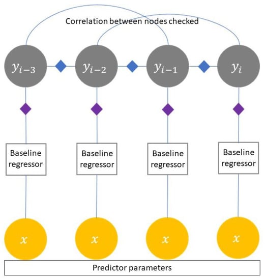
Figure 1.
Structure of the standard continuous conditional random field (CCRF).
The probabilistic density function (PDF) is an exponential model that contains features based on input and output. It is assumed that there is a connection between the labels that are adjacent to the output. The CCRF forms a connection between a point and its neighboring points. These points represent the predicted values of time unity and are generated by the conventional predictor algorithm as the baseline. Because the CCRF works in the case of regression, the baseline used is referred to as the baseline regressor. The baseline regressors that could be used in this method include the support vector machine (SVM), neural networks, or trees.
In general, the CCRF serves to strengthen probabilities for weak predictive values. In general, the CCRF model can be written as []
Here, is a set of predictive values (output), denotes the number of observed samples, and is a vector of independent random variables called predictor vectors. The function is the potential function of CCRF, which defines an interaction between every variable on a clique. A clique is a maximal subgraph, i.e., a set of vertices on a graph that has an edge for each two vertex pairs []. The function is the normalizer formula that is used to maintain the probability value between and , which is defined as
The potential function Ψ is defined as []
where is the CCRF feature variable function referred to as the association potential, is the CCRF edge feature function called the interaction potential, denotes the observation sample, and , are the contribution parameters of the feature variable and edge feature, respectively.
The feature function variable and the edge feature are the two sources of information used in CCRF. The feature function represents prior knowledge for CCRF and evaluates predictive results formed by the baseline repressors. Generally, the feature tests the prediction results by using an error evaluation function such as the mean square error (MSE). Meanwhile, the edge feature expresses the interactions between prediction values. The functions and are defined as shown in (4) and (5), respectively:
The integers and represent the number of baseline regressors and the number of similarity measurements between feature vectors, respectively. The function is an unstructured model that predicts a single output based on the input . Simply stated, is a function that maps the input to a prediction value , which is referred to as a prediction function by a baseline regressor.
3.2. DM-CCRF
The distance-to-mean continuous conditional random fields (DM-CCRF) method includes a modification made to the edge feature function of CCRF, as shown in Figure 2. It aims to improve the CCRF performance in predicting time-series data. Modifications are carried out with the assumption that there is information on the average probability of an event in the total sequence of time-series data. The prediction model belief probability that emerges is expected to increase by using this assumption. This assumption is formulated by defining a new edge feature :
Here, integer is the length of the calculated sequence, is the contribution variable of the modified edge feature, and is the average of prediction values to . The variable can be formulated as
where the integer is the sequence of events. The structure of the DM-CCRF is illustrated in Figure 3.
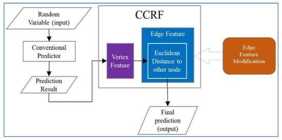
Figure 2.
Work scheme of the distance-to-mean CCRF (DM-CCRF).
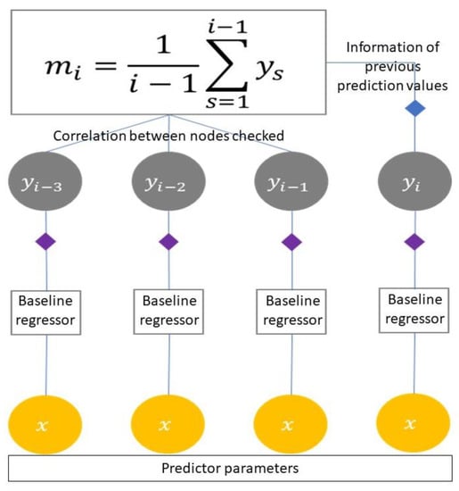
Figure 3.
Structure of the DM-CCRF.
With the formation of a new edge feature function, a DM-CCRF potential function is defined as
In the form of conditional probabilities, DM-CCRF can be written as
Thus, the form of the DM-CCRF formulation can be written as
By substituting Equations (4)–(6) into Equation (10),
In the concept of a matrix, a simplification of Equation (11) can be written as []
where
Matrix contains the contribution variable of the entire DM-CCRF feature function, is the determinant of matrix , and denotes the average predictor variable. Matrix is a diagonal matrix that contains elements
Matrix is a symmetrical matrix where the elements consist of
where is constant. Vector contains elements which are defined as
3.3. Learning and Inference in DM-CCRF
The learning process aims to select the optimum feature variable value, which will maximize the conditional probability value []. In DM-CCRF, the learning process aims to choose the optimum values of variables and such that reaches its maximum value. Given a training data , which is formed from any probability distribution [], is an input vector that corresponds to data , and is a set of predictive values that correspond to the -th data point. The value of the DM-CCRF feature variable can be estimated. A conditional logarithmic likelihood function that corresponds to the DM-CCRF model is defined from observational data, i.e.,
Equation (19) is obtained by substituting Equation (9) into Equation (18):
The learning process for training data in DM-CCRF can be written as
A stochastic gradient ascent is an algorithm that can be used to process thousands of datasets that contain hundreds of features. Therefore, the optimal value of a variable can be determined using a stochastic gradient ascent []. The partial derivatives of the conditional logarithmic function for and can be written as
It is assumed that there is a constraint that can be used to guarantee the partition function so that
where
can be integrated [,].
A constraint in Equation (24) will reach its optimum value by using a partial derivative of dan [], which can be written as
Using Equations (25)–(26), the most recent values of and for each iteration based on the gradient ascent can be calculated by using Equations (27) and (28), respectively.
where , commonly known as the learning rate, is a constant that is used to determine how significant the variables updated in each iteration are. If has an enormous value, then there is a possibility of premature convergence, whereas if has an insignificant value, then the optimization process will take a very long time to reach convergence.
In the inference process, the desired predictive value is determined []. The inference process in DM-CCRF aims to find the predictive value of for each input value X given, such that the conditional probability value reaches the maximum value. The estimated value for each optimal corresponding to the conditional probability value will be the same as the expected . The prediction value in DM-CCRF can be formulated as
4. Results and Discussion
4.1. Experimental Setup
4.1.1. Dataset
The traffic data used in this study were obtained from the Department of Transport, United Kingdom, and were collected using hundreds of sensors for 24 h. The sensors were placed on road segments and operated in a real-time scenario, resulting in an increase in size over time. The utilized data were traffic data from a Highways Agency that provides traffic flow information, average traffic speed, and average trip time for periods of 15 min []. The data were collected from 2009 to 2013. From 270,000,000 observation data points, only 2760 data points were used in the experiment, and these were located at the latitude of . These traffic data had ten attributes: source-latitude, source-longitude, destination-latitude, destination-longitude, time and date, period, vehicle speed, distance, and traffic flow. The traffic data were narrow in the morning, congested at midday, and started to plummet at the end of the day [].
The combination of automatic number plate recognition (ANPR) cameras, an in-vehicle Global Positioning System (GPS), and inductive loops was utilized to calculate the travel time and average speed attributes. Furthermore, the travel time attribute was derived from real vehicle observations and calculated using the adjacent time periods. The date attribute was converted to the number of days in one week: 1 for Monday, 2 for Tuesday, and so on. The time attribute was graded from 1 to 96, representing 00:00–24:00 per time interval. The period attribute was displayed in seconds, the vehicle speed attribute was displayed in km/h, the distance attribute was displayed in km, and the traffic flow was displayed as the number of vehicles. The process aimed to analyze the number of vehicles (traffic flow) predicted.
The cleaning process was conducted by removing the empty attributes or the attributes with values of zero. In addition, if the dataset contained missing values, then data preprocessing through imputation techniques was conducted. After the data cleaning process was complete, the remaining attributes were used as random variables with one target variable value. The target variable in question was the traffic flow prediction variable. Furthermore, the clean dataset was converted into numerical data using values between and . This was done to avoid data outliers or a huge range of data.
4.1.2. Baseline Regressor
A baseline regressor was formed before data processing with the DM-CCRF. The extreme learning machine (ELM), which is a regressor based on neural networks, was chosen as a baseline regressor. The original ELM, which is a machine learning algorithm for single-hidden layer feedforward networks (SFLNs), was proposed by Huang et al. []. Learning parameters in the ELM, namely input weights and biases from a hidden node, can be set randomly without needing to be set first in each iteration process []. As for the output on the ELM, it can be determined analytically by a simple inverse operation. The only parameter that must be defined first in the ELM is the number of hidden nodes. The ELM has a better performance than other SLFN algorithms, especially in terms of the learning process duration. In the ELM, it is assumed that any non-linear fitness function can be used as a hidden layer. Figure 4 is an illustration of the ELM, where the enlarged part shows a hidden neuron in the ELM that can load sub-hidden neurons.
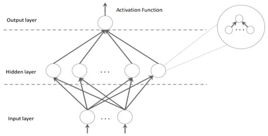
Figure 4.
Illustration of the extreme learning machine (ELM).
Several variations of ELM parameters were used to form various scenarios. These scenarios produced a baseline regressor to provide diverse quality. Furthermore, the behavior of the DM-CCRF during interaction with various baselines was observed. Each scenario was evaluated by the Mean Absolute Percentage Error (MAPE), which was used as a benchmark for the DM-CCRF. MAPE formulations can be written as
In the case of the classical regression model, one way to choose the best model is to analyze the MAPE value, where the best model can minimize the MAPE value.
4.2. Results and Discussion
Given several variations of kernel parameters with the ELM as the baseline regressor, the results of the interaction of DM-CCRF with each parameter were obtained. These are represented by regularization coefficient values. The scenarios were built on the variation of the baseline regressor, which combined the number of kernel parameters and the coefficient of regulation. The scenarios were obtained from fine-tuning ELM results. Table 1 presents the variations of ELM parameters as baseline regressors for DM-CCRF in several scenarios. Fifteen scenarios were investigated, with the smallest number of the kernel being 1 and the largest number being 1,000,000. The interval of the regularization coefficient value ranged from 1 up to 1,000,000.

Table 1.
Variation of the baseline regressor.
The evaluation of the performance of the ELM as a baseline regressor for various scenarios is shown in Figure 5. The peak MAPE value for ELM implementation, 184.76%, was given by the 15th scenario, while the lowest performance was given by the 8th scenario, . In the first scenario, ELM gave a reasonably high MAPE value, which then decreased gradually until the 8th scenario. From the 9th scenario to the 11th scenario, the MAPE value for the ELM rose, although this was not significant. It rose significantly in the 12th scenario and then stabilized with a small increase. Then, the performance of the DM-CCRF was compared with the standard CCRF and the ELM as the baseline regressor.
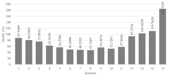
Figure 5.
The evaluation performance of several scenarios with ELM as the baseline regressor.
The same baseline regressor was implemented on the Highways Agency, United Kingdom, dataset [] for both methods. Based on Figure 6, it can be seen that the DM-CCRF and CCRF showed significant performance improvements compared with the performance of the baseline regressor for each scenario. The results provided by the standard CCRF show its ability to suppress errors obtained by the baseline regressor. Almost every scenario showed a decreasing MAPE value for the standard CCRF compared with the ELM as the baseline regressor, except for the fourth and fifth scenarios. However, the DM-CCRF provided better results than the standard CCRF in terms of minimizing MAPE values. Each scenario showed a decreased MAPE value with the DM-CCRF technique compared with the standard CCRF and ELM. These results show the superiority of the DM-CCRF compared with the standard CCRF method and ELM for traffic flow prediction.
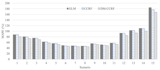
Figure 6.
Performance evaluation comparison between the DM-CCRF, CCRF, and ELM.
In Table 2, a direct comparison between the results of the DM-CCRF, standard CCRF, and the baseline regressor is displayed. For each scenario, DM-CCRF always gave superior results compared with the standard CCRF and baseline regressor. The MAPE values achieved by DM-CCRF were constantly lower than those of the standard CCRF and baseline regressor. These results show the superiority of DM-CCRF in suppressing error values for each scenario of traffic flow prediction. When the standard CCRF simply suppressed errors of compared with the baseline regression, the DM-CCRF was able to suppress errors up to .
Table 2.
Head-to-head comparison between the ELM, CCRF, and DM-CCRF.
The best performance of DM-CCRF was achieved in the 15th scenario, where the DM-CCRF provided a difference in results of compared to the regression baseline. The lowest difference to the baseline regressor, 2.365%, was obtained in the 8th scenario. Compared with the standard CCRF, DM-CCRF had the biggest difference in the 14th scenario, where the difference in error was . The smallest error, 1.299%, was found in the 8th scenario. Hence, it can be concluded that DM-CCRF provided better predictive results for the traffic flow dataset compared with the standard CCRF or ELM baseline regression.
5. Conclusions
A modification to a probability approach, continuous conditional random fields (CCRF), was proposed and implemented in the ELM and then utilized to assess highway traffic data. The modification was conducted to improve the performance of the ELM method. The experimental results showed that the proposed technique was better at suppressing the prediction error of the prediction model compared with the standard CCRF. The comparison between the ELM as the baseline regressor, the standard CCRF, and the modified CCRF was displayed. The performance evaluation of the techniques was conducted by analyzing their Mean Absolute Percentage Error (MAPE) values. The DM-CCRF was able to suppress the prediction model error twice as well as the standard CCRF method. Based on the attributes of the dataset, the DM-CCRF method was better for the prediction of highway traffic than the standard CCRF method and ELM baseline regressor.
6. Future Work
In further research, observations will be made on whether the probability of the emergence of a predictive model will continue to increase even though the belief level is not too significant. Another problem is that even though the DM-CCRF is superior to the standard CCRF, this modified method still provides a fairly large error value.
Author Contributions
Conceptualization, S.C.P. and H.R.S.; Data curation, A.W.; Formal analysis, S.C.P. and H.R.S.; Investigation, S.C.P.; Methodology, S.C.P. and H.R.S.; Resources, A.W. and W.J.; Supervision, H.R.S. and W.J.; Validation, W.J.; Visualization, S.C.P.; Writing—original draft, S.C.P.; Writing—review & editing, N.A. and H.A.W.
Funding
We would like to express our gratitude for the grant received from Universitas Indonesia and Directorate of Higher Education (2015–2017) entitled Intelligent Traffic System for Sustainable Environment, Grant No:0476/UN2.R12/HKP. 05.00/2015 in supporting this research.
Acknowledgments
Authors expressing gratitude to Sa’aadah S. Carita for verifying the mathematical equations used in this research.
Conflicts of Interest
The authors declare no conflict of interest.
References
- Board, T.R. Expanding Metropolitan Highways: Implication for Air Quality and Energy Use—Special Report 245; The National Academic Press: Washington, DC, USA, 1995. [Google Scholar]
- Chen, Y.; Guizani, M.; Zhang, Y.; Wang, L.; Crespi, N.; Lee, G.M.; Wu, T. When traffic flow prediction meets wireless big data analytics. IEEE Netw. 2019, 33, 161–167. [Google Scholar] [CrossRef]
- Lighthill, M.J.; Whitham, G.B. On kinematic waves II: A theory of traffic flow on long crowded roads. Proc. R. Soc. A Math. Phys. Eng. Sci. 1955, 229, 317–345. [Google Scholar]
- Gazis, D.C. Traffic Theory; Kluwer Academic Publishers: Norwell, MA, USA, 2002. [Google Scholar]
- Emami, A.; Sarvi, M.; Bagloee, S.A. Using Kalman filter algorithm for short-term traffic flow prediction in a connected vehicle environment. J. Mod. Transp. 2019, 27, 222–232. [Google Scholar] [CrossRef]
- Salamanis, A.; Margaritis, G.; Kehagias, D.D.; Matzoulas, G.; Tzovaras, D. Identifying patterns under bot normal and abnormal traffic conditions for short-term traffic prediction. Transp. Res. Procedia 2017, 22, 665–674. [Google Scholar] [CrossRef]
- Duan, P.; Mao, G.; Yue, W.; Wang, S. A unified STARIMA based model for short-term traffic flow prediction. In Proceedings of the 21st International Conference on Intelligent Transportation Systems (ITSC), Maui, HI, USA, 4–7 November 2018; IEEE: Piscataway, NJ, USA, 2018. [Google Scholar]
- Wang, C.; Ran, B.; Zhang, J.; Qu, X.; Yang, H. A novel approach to estimate freeway traffic state: Parallel computing and improved Kalman filter. IEEE Intell. Transp. Syst. Mag. 2018, 10, 180–193. [Google Scholar] [CrossRef]
- Wei, C.; Asakura, Y. A Bayesian approach to traffic estimation in stochastic user equilibrium networks. In 20th International Symposium on Transportation and Traffic Theory; Elsevier: Amsterdam, The Netherlands, 2013. [Google Scholar]
- Zhu, Z.; Zhu, S.; Zheng, Z.; Yang, H. A generalized Bayesian traffic model. Transp. Res. Part C 2019, 108, 182–206. [Google Scholar] [CrossRef]
- Marzano, V.; Papola, A.; Simonelli, F.; Papageorgiou, M. A Kalman filter for Quasi-Dynamic o-d flow estimation/updating. IEEE Trans. Intell. Transp. Syst. 2019, 19, 3604–3612. [Google Scholar] [CrossRef]
- Cai, L.; Zhang, Z.; Yang, J.; Yu, Y.; Zhou, T.; Qin, J. A noise-immune Kalman filter for short-term traffic flow forecasting. Phys. A 2019, 536, 122601. [Google Scholar] [CrossRef]
- Duan, P.; Mao, G.; Zhang, C.; Kang, J. A trade-off between accuracy and complexity: Short-term traffic flow prediction with spational-temporal correlations. In Proceedings of the 21th International Conference on Intelligent Transportation Systems (ITSC), Maui, HI, USA, 4–7 November 2018; IEEE: Piscataway, NJ, USA, 2018. [Google Scholar]
- Alghamdi, T.; Elgazzar, K.; Bayoumi, M.; Sharaf, T.; Shah, S. Forecasting traffic congestion using ARIMA modeling. In Proceedings of the 15th International Wireless Communications & Mobile Computing Conference (IWCMC), Tangier, Morocco, 24–28 June 2019; IEEE: Piscataway, NJ, USA, 2019. [Google Scholar]
- Chu, K.C.; Saigal, R.; Saitou, K. Real-time traffic prediction and probing strategy for Lagrangian traffic data. IEEE Trans. Intell. Transp. Syst. 2019, 20, 497–506. [Google Scholar] [CrossRef]
- Tu, Q.; Cheng, L.; Li, D.; Ma, J.; Sun, C. Stochastic transportation network considering ATIS with the information of environmental cost. Sustainability 2018, 10, 3861. [Google Scholar] [CrossRef]
- Zantalis, F.; Koulouras, G.; Karabetsos, S.; Kandris, D. A review of machine learning and IoT in smart transportation. Future Internet 2019, 11, 94. [Google Scholar] [CrossRef]
- Fouladgar, M.; Parchami, M.; Elmasri, R.; Ghaderi, A. Scalable deep traffic flow neural networks for urban traffic congestion prediction. In Proceedings of the International Joint Conference on Neural Network (IJCNN), Anchorage, AK, USA, 14–19 May 2017; pp. 2251–2258. [Google Scholar]
- Chen, Y.; Chen, F.; Ren, Y.; Wu, T.; Yao, Y. DeepTFP: Mobile Time Series Data Analytics Based Traffic Flow Prediction; MobiCom: Ulaanbaatar, Mongolia, 2017; pp. 537–539. [Google Scholar]
- Tian, Y.; Zhang, K.; Li, J.; Lin, X.; Yang, B. LSTM-based traffic flow prediction with missing data. Neurocomputing 2018, 318, 297–305. [Google Scholar] [CrossRef]
- Yang, B.; Sun, S.; Li, J.; Lin, X.; Tian, Y. Traffic flow prediction using LSTM with feature enhancement. Neurocomputing 2019, 332, 320–327. [Google Scholar] [CrossRef]
- Wen, F.; Zhang, G.; Sun, L.; Wang, X.; Xu, X. A hybrid temporal association rules mining method for traffic congestion prediction. Comput. Ind. Eng. 2019, 130, 779–787. [Google Scholar] [CrossRef]
- Lopez-Martin, M.; Carro, B.; Sanchez-Esguevillas, A. Neural network architecture based on gradient boosting for IoT traffic prediction. Future Gener. Comput. Syst. 2019, 100, 656–673. [Google Scholar] [CrossRef]
- Lin, L.; Handley, J.C.; Gu, Y.; Zhu, L.; Wen, X.; Sadek, A.W. Quantifying uncertainty in short-term traffic prediction and its application to optimal staffing plan development. Transp. Res. Part C 2018, 92, 323–348. [Google Scholar] [CrossRef]
- Hou, Q.; Leng, J.; Ma, G.; Liu, W.; Cheng, Y. An adaptive hybrid model for short-term urban traffic flow prediction. Phys. A 2019, 527, 121065. [Google Scholar] [CrossRef]
- Jia, R.; Jiang, P.; Liu, L.; Cui, L.; Shi, Y. Data driven congestion trends prediction of urban transportation. IEEE Int. Things J. 2018, 5, 581–591. [Google Scholar] [CrossRef]
- Li, C.; Anavatti, S.G.; Ray, T. Short-term traffic flow prediction using different techniques. In Proceedings of the IECON 2011-37th Annual Conference of the IEEE Industrial Electronics Society, Melbourne, Australia, 7–10 November 2011. [Google Scholar]
- Chi, Z.; Shi, L. Short-term traffic flow forecasting using ARIMa-SVM algorithm and R. In Proceedings of the 5th International Conference on Information Science and Control Engineering, Zhengzhou, China, 20–22 July 2018; IEEE: Piscataway, NJ, USA, 2018. [Google Scholar]
- Li, K.L.; Zhai, C.J.; Xu, J.M. Short-term traffic flow prediction using a methodology based on ARIMA and RBF-ANN. In Proceedings of the Chinese Automation Congress (CAC), Jinan, China, 20–22 October 2017; IEEE: Piscataway, NJ, USA, 2017. [Google Scholar]
- Koller, D.; Friedman, N. Probabilistic Graphical Models: Principles and Techniques; The MIT Press: Cambridge, MA, USA, 2010; p. 3. [Google Scholar]
- Xing, Y.M.; Ban, X.J.; Liu, R.Y. A short-term traffic flow prediction method based on Kernel Extreme Learning Machine. In Proceedings of the International Conference on Big Data and Smart Computing, Shanghai, China, 15–17 January 2018; IEEE: Piscataway, NJ, USA, 2018. [Google Scholar]
- Zu, W.; Xia, Y. Back propagation bidirectional extreme learning machine for traffic flow time series prediction. Neural Comput. Appl. 2019, 31, 7401–7417. [Google Scholar] [CrossRef]
- Ban, X.; Guo, C.; Li, G. Application of extreme learning machine on large scale traffic congestion prediction. In Proceedings of ELM-2015 Volume 1; Springer: Cham, Switzerland, 2015; pp. 293–305. [Google Scholar]
- Zhang, Q.; Jian, D.; Xu, R.; Dai, W.; Liu, Y. Integrating heterogeneous data sources for traffic flow prediction through extreme learning machine. In Proceedings of the IEEE International Conference on Big Data (BIGDATA), Boston, MA, USA, 11–14 December 2017. [Google Scholar]
- Xing, Y.; Ban, X.; Liu, X.; Shen, Q. Large-scale traffic congestion prediction based on the symmetric extreme learning machine cluster fast learning method. Symmetry 2019, 11, 730. [Google Scholar] [CrossRef]
- Yang, H.F.; Dillon, T.S.; Chang, E.; Chen, Y.P.P. Optimized configuration of exponential smoothing and extreme learning machine for traffic flo9w forecasting. IEEE Trans. Ind. Inform. 2019, 15, 23–34. [Google Scholar] [CrossRef]
- Feng, W.; Chen, H.; Zhang, Z. Short-term traffic flow prediction based on wavelet function and extreme learning machine. In Proceedings of the 7th Data Driven Control and Learning Systems Conference (DDCLS), Enshi, China, 25–27 May 2018; IEEE: Piscataway, NJ, USA, 2018. [Google Scholar]
- Radosavljevic, V.; Vucetic, S.; Obradovic, Z. Continuous conditional random fields for regression in remote sensing. In Proceedings of the European Conference on Artificial Intelligence (ECAI), Lisbon, Portugal, 16–20 August 2010; pp. 809–814. [Google Scholar]
- Baltrusaitis, T.; Banda, N.; Robinson, P. Dimensional affect recognition using continuous conditional random. In Proceedings of the IEEE International Conference on Automatic Face and Gesture Recognition, Shanghai, China, 22–26 April 2013. [Google Scholar]
- Baltrusaitis, T. Automatic Facial Expression Analysis; University of Cambridge: Cambridge, UK, 2014. [Google Scholar]
- Baltrusaitis, T.; Robinson, P.; Morency, L. Continuous conditional neural fields for structured regressions. In Proceedings of the European Conference on Computer Vision, Zurich, Switzerland, 5–12 September 2014; pp. 1–16. [Google Scholar]
- Fu, K.; Gu, I.Y.H.; Yang, J. Saliency detection by fully learning a continuous conditional random filed. IEEE Trans. Multimed. 2017, 19, 1531–1544. [Google Scholar] [CrossRef]
- Xu, D.; Ricci, E.; Ouyang, W.; Wang, X.; Sebe, N. Multi-scale continuous CRFs as sequential deep networks for monocular depth estimation. In Proceedings of the IEEE Conference on Computer Vision and Pattern Recognition, Honolulu, HI, USA, 21–26 July 2017. [Google Scholar]
- Banda, N.; He, L.; Engelbrecht, A. Bio-acoustic emotion recognition using continuous conditional recurrent fields. In Proceedings of the IEEE Symposium Series on Computational Intelligence (SSCI), Honolulu, HI, USA, 27 November–1 December 2017. [Google Scholar]
- Zhou, H.; Ouyang, W.; Cheng, J.; Wang, X.; Li, H. Deep continuous conditional random fields with asymmetric inter-object constraints for online multi-object tracking. IEEE Trans. Circuits Syst. Video Technol. 2018, 29, 1011–1022. [Google Scholar] [CrossRef]
- Imbrasaite, V.; Baltrusaitis, T.; Robinson, P. CCNF for continuous emotion tracking in music: Comparison with CCRF and relative feature representation. In Proceedings of the IEEE International Conference on Multimedia and Expo Workshops (ICMEW), Chengdu, China, 14–18 July 2014; pp. 1–6. [Google Scholar]
- Qin, T.; Liu, T.; Zhang, X.; Wang, D.; Li, H. Global ranking using continuous conditional random fields. In Advances in Neural Information Processing Systems; Neural Information Processing Systems (NIPS): Vancouver, BC, Canada, 2009; pp. 1281–1288. [Google Scholar]
- Gewali, U.B.; Monteiro, S.T. A tutorial on modeling and inference in undirected graphical models for hyperspectral image analysis. Int. J. Remote Sens. 2018, 39, 1–40. [Google Scholar] [CrossRef]
- Ristovski, K.; Radosavljevic, V.; Vucetic, S.; Obradovic, Z. Continuous conditional random fields for efficient regression in large fully connected graphs. In Proceedings of the Twenty-Seventh AAAI Conference on Artificial Intelligence, Washington, DC, USA, 14–18 July 2013. [Google Scholar]
- UK Highways Agency. Highways Agency Network Journey Time and Traffic Flow Data. Retrieved June 12, 2014, from Data.go.uk. Available online: https://data.gov.uk/dataset/dc18f7d5-2669-490f-b2b5-77f27ec133ad/highways-agency-network-journey-time-and-traffic-flow-data (accessed on 2 December 2019).
- Wibisono, A.; Jatmiko, W.; Wisesa, H.A.; Hardjono, B.; Mursanto, P. Traffic big data prediction and visualization using Fast Incremental Model Trees-Drift Detection (FIMT-DD). Knowl. Based Syst. 2016, 93, 33–46. [Google Scholar] [CrossRef]
- Huang, G.B.; Zhu, Q.Y.; Siew, C.K. Extreme learning machine: A new learning scheme of feedforward neural networks. In Proceedings of the 2004 International Joint Conference on Neural Networks, Budapest, Hungary, 25–29 July 2004; Volume 2, pp. 985–990. [Google Scholar]
- Ding, S.; Xu, X.; Nie, R. Extreme learning machine and its applications. Neural Comput. Appl. 2013, 25, 549–556. [Google Scholar] [CrossRef]
© 2019 by the authors. Licensee MDPI, Basel, Switzerland. This article is an open access article distributed under the terms and conditions of the Creative Commons Attribution (CC BY) license (http://creativecommons.org/licenses/by/4.0/).