Hybrid Optimization Algorithm for Bayesian Network Structure Learning


Software School, Yunnan University, Kunming 650091, China
*
Authors to whom correspondence should be addressed.
Information 2019, 10(10), 294; https://doi.org/10.3390/info10100294
Submission received: 17 August 2019
/
Revised: 17 September 2019
/
Accepted: 21 September 2019
/
Published: 24 September 2019
Abstract
:Since the beginning of the 21st century, research on artificial intelligence has made great progress. Bayesian networks have gradually become one of the hotspots and important achievements in artificial intelligence research. Establishing an effective Bayesian network structure is the foundation and core of the learning and application of Bayesian networks. In Bayesian network structure learning, the traditional method of utilizing expert knowledge to construct the network structure is gradually replaced by the data learning structure method. However, as a result of the large amount of possible network structures, the search space is too large. The method of Bayesian network learning through training data usually has the problems of low precision or high complexity, which make the structure of learning differ greatly from that of reality, which has a great influence on the reasoning and practical application of Bayesian networks. In order to solve this problem, a hybrid optimization artificial bee colony algorithm is discretized and applied to structure learning. A hybrid optimization technique for the Bayesian network structure learning method is proposed. Experimental simulation results show that the proposed hybrid optimization structure learning algorithm has better structure and better convergence.
1. Introduction
The birth of the first computer in 1946 marked the creation of a real tool with which humans were able to simulate human thinking. In 1956, artificial intelligence was officially proposed, and since then, it has made great progress. In the 1970s and 1980s, the “expert system” became the focus of research in the field of artificial intelligence. By collecting the experience and knowledge of experts in various fields, summing these up as operating rules, and then inputting the obtained rules to a computer, computers are able to solve problems encountered in the field. However, this rule-based expert system does not have the ability to learn. When a rule changes, such as the need to replace an old rule with a new rule, the expert system does not automatically adjust. In 1988, the Turing Award winner Jedea Pearl first proposed the Bayesian network [1]. Compared with the expert system based on empirical knowledge, the Bayesian network solves the uncertainty problem, especially when solving complex problems, making it more effective and intuitive. Today, the data shows an explosive growth trend. The traditional method of analyzing knowledge and inducting experience to make decisions cannot meet the needs of social development. The great advantages of Bayesian networks in solving uncertainty problems have made them central to the study of intelligence, data mining, and machine learning, as well as to many fields involving decision-making, diagnosis, and evaluation [2].
Bayesian network structure learning includes structure learning and parametric learning [3]. Structure learning is the premise and basis of parametric learning, and it is also the core of Bayesian network learning research. For high-dimensional data sets, which are currently exploding in various fields, there are thousands of nodes involved, making the corresponding Bayesian network structure very complicated. Learning the Bayesian network structure from the data becomes a non-deterministic polynomial (NP)-hard [4] question. Therefore, one of the main challenges of Bayesian network research is to find an effective structure learning method to learn an optimal structure from complex and high-dimensional data sets in a reasonable time frame.
2. Bayesian Network Structure Learning Overview
2.1. Bayesian Network and Structure Model
A Bayesian network (BN) is a graph model [5] that describes the correlation between random variables in a probabilistic way. In the graph model, nodes represent variables, directed edges represent “causal relationships” between variables, parent nodes represent “causes”, child nodes represent “results”, and child nodes store their conditional probabilities distributed relative to the parent node. The Bayesian network can be expressed as (G, Θ), and the Bayesian network structure G = (V, E) is a directed acyclic graph (DAG) [6,7] that represents the relationships of the nodes, where V = {V1, V2, ..., Vn} is a collection of nodes in a Bayesian network, and E represents a collection of directed edges joined by nodes. Θ is a Bayesian network parameter that represents the conditional probability table for all nodes under their parent node conditions. Figure 1a shows the complete Bayesian network constructed using the Asia data set [8]. The probability parameters of each node and the correlation between nodes can be seen in the figure. If smoking points to lung cancer, it means that smoking causes the occurrence of lung cancer. The smoking node is the parent node and the lung cancer node is the child node.
Bayesian network structure learning is shown in Figure 1b. The 1 and 0 in the table indicate the possible states of the node, with 1 indicating true and 0 false. A network structure is constructed by using the structure learning algorithm to analyze the sample data in the table and find the dependencies between nodes. The purpose of structure learning is to find an optimal Bayesian network structure (which is most consistent with the sample set) by learning the prediction data set. According to whether there is missing training data, structure learning is also divided into complete data structure learning and missing data structure learning. In this paper, we mainly studied the Bayesian network structure learning problem under the complete training set.
2.2. Main Structure Learning Method
For the training data set D composed of a set of random variables V = {V1, V2, ..., Vn}, the structure learning is to find the corresponding DAG graph structure. At this time, the number of nodes is n, f(n) is the number of directed acyclic graphs composed of n nodes; Robinson [9] proves that there is the following relationship between the number of DAG f(n) and the number of nodes n:
It can be seen from Equation (1) that as the number of nodes increases, the number of DAG increases exponentially. Obviously, for this NP-hard problem, it is unrealistic to manually construct a Bayesian network structure. To this end, the researchers propose a number of different structure learning algorithms. The research methods of these algorithms are broadly divided into constraint-based [10] structure learning methods and score-and-search-based methods [11]. The score-and-search-based method selects a scoring function to evaluate the similarity between the BN structure and the actual structure, and performs multiple iterative searches through the search algorithm to find the structure with the highest score. This structure learning method regards the network structure learning problem as an optimization problem, and the scoring function corresponds to the fitness function in the optimization problem. This paper adopted this structure learning method.
The structure learning mathematical model based on the search score is shown in Equation (2):
where f (G, D) represents the network structure scoring function of data set D, G’ represents all possible structure spaces, and C represents constraints (i.e., the searched structure graph satisfies being termed acyclic).
In Equation (3), since the data set is given, f(D) is a fixed value, the objective of structure learning is to find an optimal network structure G*, expressed as
In structure learning based on search score, in order to find the optimal network structure G*, it is necessary to calculate the score f(G, D) according to the given training data D and its possible structure G; the scoring function is needed at this time. Some commonly used scoring functions are the Bayesian Dirichlet equivalence (BDeu) score [12], Log-Likelihood (LL) score [13], Akaike’s information criterion (AIC) score [13], Bayesian information criterion (BIC) score [14], and so on. The BIC score fully considers the complexity of the structural parameters, and also considers the storage bytes of the training samples, making it more suitable for the training data of smaller samples such as the experiments herein. Therefore, we use the BIC score as a standard function to measure the Bayesian network structure in this chapter. The BIC score can usually be expressed as
The input parameters are the structure matrix G and the data matrix D. n is the number of nodes, ri is the number of nodes in the Vi state (the number of possible values), and qi is the number of parent nodes of node Vi. m is the number of samples, and mijk is the number of samples in which the node Vi takes the value k and the parent node takes the value j.
As mentioned above, the problem of learning the network from the data is generally considered to be an NP-hard optimization problem, so it is necessary to find an efficient search algorithm; to this end, the heuristic algorithm has high search efficiency and is often used to find the best network structure in structure learning. This type of search method mainly includes the K2 algorithm [15], the simulated annealing algorithm [15], the hill climbing algorithm [16], and evolutionary algorithm methods. The evolutionary algorithm is simple to implement, and the global search ability is stronger. Compared with other traditional search methods, the global information can be more comprehensively utilized, and the dependence on the optimization function is small. Therefore, the network structure learned by the structure learning method based on the evolutionary algorithm has a smaller difference with the real structure, and can converge to a better structure more quickly, the convergence itself is also better [17,18,19,20].
3. Hybrid Optimization Artificial Bee Colony Algorithm for Bayesian Network Structure Learning
The structure learning method based on the artificial bee colony algorithm (ABC) [21] treats the process of learning Bayesian network structure from a data set as the process of a bee colony searching for a food source. The directed acyclic graph is transformed into matrix form, and then the finding of the optimal network structure is transformed into the finding of an optimal matrix, the computer can thereafter perform matrix operations. Each possible Bayesian network structure is regarded as a food source for calculation, the correspondence between them is shown in Table 1.
In structure learning based on search scoring, the structure map is usually represented by a matrix of 0 or 1, and the solution search space is discrete. Although the artificial bee colony algorithm can solve the optimization problem of continuous function well, it fails when it encounters the discrete domain problem. Therefore, on the basis of a multi-group artificial bee colony algorithm based on cuckoo algorithm (CMABC) and knowledge of Bayesian networks, this paper proposed a Bayesian network structure learning method based on discrete CMABC algorithm (CMABC-BNL).
3.1. Problem Abstraction
In order to transform the directed acyclic graph DAG in a Bayesian network into a computer-understandable representation, we used the same matrix coding form as in Reference [22]. Assuming that the number of nodes in the BN network is n, the DAG graph composed of the n nodes can be represented as an n × n matrix A according to the relationship between the nodes, and the elements aij in A are defined as follows:
Figure 2 shows the process of converting a DAG diagram into an adjacent matrix.
In CMABC-BNL, the structure diagram is uniquely determined in the form of a matrix, as shown in Figure 2; the DAG diagram is converted to A1, and this matrix consists of n2 elements. Since every possible structure is seen as a food source, the structure diagram can be used to obtain an n2-dimensional food source through the following transformation process:
3.2. Algorithm Description
3.2.1. Initialization Phase
The BN structure is a discrete space composed of 0 or 1. We generate SN food sources with an initial value of 0 or 1 through the Bernoulli Process [23]; the initial process of each food source Xij is shown in Equation (8):
where Xij = (Xi1, Xi2, ..., XiD) represents the i-th food source, i = 1, 2, ..., SN, j = 1, 2, ..., D, D = n2 is the dimension in the solution space, rand is a random number between [0,1].
3.2.2. Fitness Function
In CMABC-BNL, Equation (5) is chosen as a standard function to measure the structure of the Bayesian network. The value obtained by using the BIC score evaluation structure is usually negative, and if the BIC value is larger, the difference between the network structure and the real structure is smaller. In the artificial bee colony algorithm, the fitness value indicates the quality of the food source, usually expressed by a positive value: if the fitness value is larger, the quality of the food source is better. Therefore, this paper redefines the fitness function as
3.2.3. Employed Foragers
In the swarm intelligence optimization algorithm, in order to find the global optimal solution, more resources (groups) should be allocated to searching and developing the food-rich areas. In general, the probability of finding a better solution near some better solutions is bigger. Therefore, this paper aims to divide the population into elite subgroups, ordinary subgroups, and vulnerable subgroups by the richness of food sources (fitness values) without loss of population diversity. Since the search space for structure learning problems is discrete, the search equations for continuous problems cannot satisfy the solution’s needs. We combined the idea of cross-variation in the differential evolution algorithm [24,25] to adjust the search ability of the three subgroups with different mutations and crossover operators.
(1) Variation Behavior
Different mutation operators were used to control the variation behavior of different populations. The variation of the three subgroups is as follows:
vulnerable subgroups:
ordinary subgroups:
elite subgroups:
where rand is a random number between [0,1], p ≠ i, Xp(t) is a food source randomly selected from all populations, and Xgb(t) is the current optimal food source. M(·) is a Bswap mutation [26] operation as shown in Algorithm 1. Taking the elite subgroup as an example, when rand is greater than 0.4, the individual will choose Xgb, j(t) to mutate, obtain, and use the information of the current optimal food source, and find a better food source more quickly. The optimization process tends to cause the algorithm to fall into a local optimum. Conversely, selecting Xp(t) to mutate and selecting random individuals to increase the randomness of the search process can enhance the ability of the algorithm to jump out of the local optimum. We used the same design idea in the CMABC algorithm to design different mutation modes for the three subgroups to balance the global search and local search ability of each subgroup, and enhance the optimization performance of the algorithm while maintaining biodiversity.
| Algorithm 1. Bswap Mutation |
| Input: food source Xi |
| Output: food source after mutation operation M(Xi) |
| 1 Select two random values in [1, D], u, v; |
| 2 If Xiu(t) = Xiv(t), then Xiu(t) = (Xiu(t) + 1) mod 2; |
| Otherwise, Xiu(t) = (Xiu(t) + 1) mod 2, Xiv(t) = (Xiv(t) + 1) mod 2 |
(2) Crossover Behavior
After the food source Xi(t) is mutated to Vi(t), Xi(t) and Vi(t) are cross-interleaved by a crossover operation to produce a new food source Xi’(t). The crossover operation is as shown in Equation (13):
where j = 1, 2, ..., D. rj is a random number of each dimension j between [0,1].
(3) Choice Behavior
We used the same greedy selection strategy as the ABC algorithm to select new and old food sources and leave the food source with a high fitness value.
3.2.4. Followers
In CMABC-BNL, the Follower will calculate the follow-up probability according to the fitness of the food source, then they will select the employed foragers to follow and search in the neighborhood according to the probability. We used the same roulette selection probability formula as in Equation (4) to calculate the probability pi(t) of the follower. If pi(t) > rand [0,1], the follower will select the food source and search and update using Equation (11) and Equation (13).
3.2.5. Scouter
If the quality (fitness value) of the food source does not increase after a limited iterative search, the corresponding employed foragers will be discarded as scouters and the food source will be updated. We use Equation (11) to update the food source and change the value of the step size scaling factor α to α = O(L/10) to make the food source update more efficient. Since the position of the food source is composed of discrete points 0 or 1, we need to round up the newly generated food source position with the following formula:
3.2.6. Structure Correction
The Bayesian network is a directed acyclic graph model. The existence condition of this model is that there is no “closed loop” in the structure. However, in CMABC-BNL, the structure changes according to the progress of the search process. Multiple 0,1 transformations of nodes lead to edge changes (deletion, joining, or inversion), and a “ring” may occur there in the structure. At this time, the structure searched cannot be used as the optimal Bayesian network structure regardless of the score. For example, in Figure 3, matrix A1 corresponds to food source Xi. When a new food source Vi is searched, a51 in the corresponding matrix A2 changes from 0 to 1, and the corresponding structure forms a directed edge from V to D which makes the BN structure corresponding to the new food source produce a ring “V, S, B”.
In order to avoid the occurrence of illegal structures to invalidate the algorithm, we need to check whether the structure has a ring, and “break” the ring structure once a new structure (new food source) appears. In this paper, inspired by the nodes in the depth-first search (DFS) which are color-coded, the color being used to judge the state of the node, a marked depth-first search (marked DFS, MDFS) strategy is proposed to search the structure of the ring and also fix this belt loop structure. The specific structure correction steps are as follows:
Step 1: Convert food source Xi into corresponding matrix Ai.
Step 2: Initialize all nodes to grey, i = 1.
Step 3: Select node ai as the initial node, use depth-first search for its descendant nodes, and mark the descendant nodes as white.
Step 4: When node ai completes the DFS search, it is judged whether a1 will be white. If it is white, it means that there is a ring structure, and the edges that make up the ring are marked as black.
Step 5: If there is a black ring, randomly delete one of the black edges and update the matrix Ai. i = i + 1.
Step 6: Determine if i is less than n, and if so, execute Step 3, otherwise, execute Step 7.
Step 7: Convert Ai to food source Xi.
3.3. Algorithm Flow
In order to better explain the process of the algorithm, we introduced algorithm 2 to make a description.
| Algorithm 2. CMABC-BNL |
| Input: Training data D Output: Optimal food source (structure)
|
3.4. Algorithm Complexity Analysis
As shown in Algorithm 2, the number of employed foragers and followers is SN, the number of nodes in the structure diagram is n, the dimension of the food source is D = n × n, the number of samples is m, and the number of iterations is M.
In the structure correction process, for a structure with n nodes, it is generally necessary to traverse all the elements in the structure diagram once, so the time complexity of the structure correction is O(n2); the process of converting the structure diagram into a food source is linear. Therefore, the time complexity is O(n2).
In one iteration, the population division, the employed foragers, the followers, and the scouter are serial. The time complexity of population partitioning is O(SN); for employed foragers, this paper divided the employed foragers into three subgroups, and the mutating and crossover behavior of a single employed foragers to produce new food sources is linear, so the complexity is O(n2). The search process of each type of subgroup is independent, and the complexity of calculating the food source fitness value is O (M × n2), so the time complexity of the SN employment bee search process is O(SN × m × n2); followers select the food source for searching. In the worst case, all followers are selected for neighborhood search, so the time complexity of SN followers is O (SN × m × n2). When a food source is not updated after a limit iteration, the employed foragers becomes a scouter. At this time, the time complexity of the scouter to update the food source is O(n2), so in the worst case, the SN employed foragers are converted into the scouter, the time complexity is O (SN × n2).
In summary, the time complexity of CMABC-BNL is O (SN × m × n2+SN × m × n2+SN × n2) = O (SN × m × n2).
3.5. Simulation Experiment and Result Analysis
In this paper, three classical Bayesian network data sets, ASIA, ALARM and INSURANCE [27], were selected, as shown in Table 2. Among them, ASIA is used for medical diagnosis of tuberculosis and cancer models, ALARM is used to monitor patients’ alarm systems, and INSURANCE is used for automotive industry insurance risk assessment. We performed a data set design comparison experiment for three Bayesian randomly selected different sample numbers.
In order to test the effectiveness and performance of CMABC-BNL, 20 independent experiments were used as the experimental sample to count objective function values (fitness values), Hamming distance (SHD), and average execution time (Ext). SHD is the operand needed to convert from the current structure to the correct structure, which is used to measure the difference between the learned structure and the real structure. Ext represents the time required to learn the final structure, reflecting the convergence of the algorithm. Table 3 shows the results of averaging experimental data after CMABC-BNL was run 10 times independently under each data set.
Table 3 compares the data of CMABC-BNL under different data sets. Figure 4 and Figure 5 show the ASIA network obtained under the standard ASIA network and 500 sample sets, respectively. As can be seen from the chart, for the ASIA data set, in the worst case, the structure learned by CMABC-BNL had only one reverse side compared with the real structure. Figure 6 and Figure 7 show the ALARM network obtained under the standard ALARM network and the 5000 data sets, respectively. As can be seen from the figure, for the ALARM data set, in the best case, the structure obtained by learning had only two missing sides and one reverse side compared with the real structure. As for INSURANCE, it can be seen that its data was very similar to ALARM. At the same time, the effect of learning the number of samples of 5000 was obviously better than that of the sample with 500 samples, and the convergence speed was also faster. This also indicated that a large sample training set could be used to improve the performance of the algorithm.
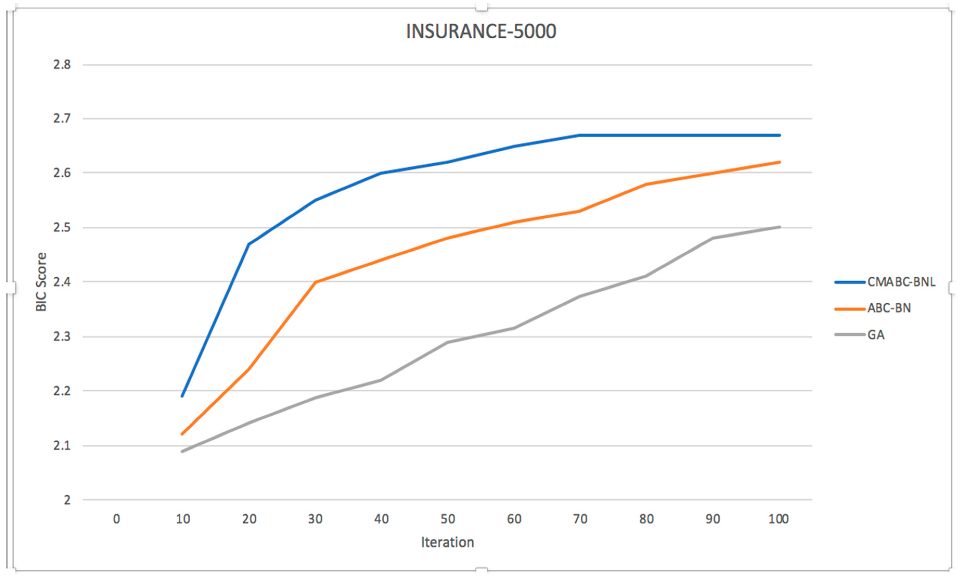
To better illustrate the performance advantages of CMABC-BNL, the algorithm was compared with genetic algorithms (GA) [22], Bayesian network structure learning based on artificial bee colony algorithm (ABC-BN) [28], Bayesian network construction algorithm using PSO (BNC-PSO) [29] and GES [30] under 1000 data sets and 5000 data sets. The population of each algorithm was set to 50, and the maximum number of iterations was set to 100. At the same time, we also introduced the F1 value as the criterion. The F1 value is the harmonic mean between the recall rate and the accuracy rate. The larger the F1 value, the better the classification performance.
It can be seen from Table 4 and Figure 8, Figure 9 and Figure 10 that CMABC-BNL was significantly better than the other two algorithms. In the ASIA network, ABC-BN and BNC-PSO ran at a lower speed, and GA reached a local optimum with fewer iterations. In ALARM and INSURANCE, the convergence of ABC-BN was better than that of CMABC, which indicated that for the more complex Bayesian network structure, the convergence accuracy of ALARM was significantly improved when there was no significant difference in convergence speed between ALARM and ABC-BN. For a simpler structure, it took less time to learn, and although some execution efficiency was sacrificed, the convergence accuracy could be significantly improved within an acceptable range. GES used the equilibrium class as the state of greedy search, which also made it require fewer execution iterations. However, the structure learned was generally larger than the actual one. In order to show the results more clearly, two relatively interfering algorithms GES and BNC-PSO were removed in the following line chart. This showed the superiority of the CMABC-BNL algorithm more clearly. In addition, it could be seen from the F1 value that in the ASIA network, the value of CMABC-BNL was only slightly lower than that of BNC-PSO. In ALARM and INSURANCE, the F1 value of CMABC-BNL showed better performance. In summary, CMABC-BNL had better performance advantages and practicability than the other two algorithms.
4. Conclusions
This paper proposed a Bayesian network structure learning algorithm based on the discrete CMABC algorithm. Firstly, the process of finding the optimal network structure was regarded as the process of finding the optimal food source, and the Bayesian network structure learning problem was abstracted into the discrete domain problem. Then, by combining the crossover and mutation operators in the differential evolution algorithm, preserving the idea of multiple groups in CMABC, designing a multi-group search strategy, and “rounding up” the food source update strategy based on Levy flight in the CMABC algorithm, it could be applied to discrete problems. In addition, regarding illegal structures in the structure learning problem, a marked depth-first search strategy was proposed to modify the structure of the ring. Finally, we carried out a complexity analysis of CMABC, comparing it with GA and ABC-BN on two data sets with different sample numbers and a large difference in node number. The experimental results showed that CMABC-BNL had certain performance advantages and application value, and there was also space for CMABC-BNL to learn from other similar algorithms.
Author Contributions
Conceptualization, X.S.; funding acquisition, Y.S.; project administration, Q.C.; software, H.K.; writing—original draft, C.C.; writing—review and editing, L.W.
Funding
This research was funded by the National Natural Science Foundation of China (No.61663046 and No. 61876166), and the Open Foundation of Key Laboratory of Software Engineering of Yunnan Province (No. 2015SE204).
Conflicts of Interest
The authors declare no conflict of interest.
References
- Friedman, N.; Dan, G.; Goldszmidt, M. Bayesian Network Classifiers. Mach. Learn. 1997, 29, 131–163. [Google Scholar] [CrossRef] [Green Version]
- Taheri, S.; Mammadov, M. Structure Learning of Bayesian Networks using Global Optimization with Applications in Data Classification. Optim. Lett. 2015, 9, 931–948. [Google Scholar] [CrossRef]
- Pearl, J. Probabilistic reasoning in intelligent systems: Networks of plausible inference. J. Philos. 1988, 88, 434–437. [Google Scholar]
- Chickering, D.M.; Dan, G.; Heckerman, D. Learning Bayesian Networks is NP-Hard. Networks 1994, 112, 121–130. [Google Scholar]
- Pinto, P.C.; Runkler, T.A. Using a local discovery ant algorithm for Bayesian network structure learning. IEEE Trans. Evol. Comput. 2009, 13, 767–779. [Google Scholar] [CrossRef]
- Balasubramanian, A.; Levine, B.; Venkataramani, A. DTN routing as a resource allocation problem. ACM Sigcomm Comput. Commun. Rev. 2007, 37, 373–384. [Google Scholar] [CrossRef] [Green Version]
- Geng, H.J.; Shi, X.G.; Wang, Z.L.; Yin, X.; Yin, S.P. Energy-efficient Intra-domain Routing Algorithm Based on Directed Acyclic Graph. Comput. Sci. 2018, 45, 112–116. [Google Scholar]
- Lauritzen, S.L.; Spiegelhalter, D.J. Local Computations with Probabilities on Graphical Structures and their Application to Expert Systems. J. R. Stat. Soc. 1988, 50, 157–224. [Google Scholar] [CrossRef]
- Robinson, R.W. Counting unlabeled acyclic digraphs. In Proceedings of the Fifth Australian Conference on Combinatorial Mathematics V, Melbourne, Australia, 24–26 August 1976; Springer: Berlin/Heidelberg, Germany, 1977; pp. 28–43. [Google Scholar]
- Schellenberger, J.; Que, R.; Fleming, R.M.; Thiele, I.; Orth, J.D.; Feist, A.M.; Zielinski, D.C.; Bordbar, A.; Lewis, N.E.; Rahmanian, S. Quantitative prediction of cellular metabolism with constraint-based models: The COBRA Toolbox v2.0. Nat. Protoc. 2011, 6, 1290–1307. [Google Scholar] [CrossRef] [PubMed]
- Lee, C.; van Beek, P. Metaheuristics for Score-and-Search Bayesian Network Structure Learning. In Proceedings of the 30th Canadian Conference on Artificial Intelligence, Canadian AI 2017, Edmonton, AB, Canada, 16–19 May 2017. [Google Scholar]
- Campos, L.M.D. A Scoring Function for Learning Bayesian Networks based on Mutual Information and Conditional Independence Tests. J. Mach. Learn. Res. 2006, 7, 2149–2187. [Google Scholar]
- Akaike, H. A New Look at the Statistical Model Identification. Autom. Control. IEEE Trans. 1974, 19, 716–723. [Google Scholar] [CrossRef]
- Anděl, J.; Perez, M.G.; Negrao, A.I. Estimating the dimension of a linear model. Ann. Stat. 1981, 17, 514–525. [Google Scholar]
- Kirkpatrick, S. Optimization by simulated annealing: Quantitative studies. J. Stat. Phys. 1984, 34, 975–986. [Google Scholar] [CrossRef]
- Heckerman, D.; Dan, G.; Chickering, D.M. Learning Bayesian Networks: The Combination of Knowledge and Statistical Data. Mach. Learn. 1995, 20, 197–243. [Google Scholar] [CrossRef]
- An, N.; Teng, Y.; Zhu, M.M. Bayesian network structure learning method based on causal effect. J. Comput. Appl. 2018, 35, 95–99. [Google Scholar]
- Cao, J. Bayesian Network Structure Learning and Application Research. Available online: http://cdmd.cnki.com.cn/Article/CDMD-10358-1017065349.htm (accessed on 22 September 2019). (In Chinese).
- Gao, X.G.; Ye, S.M.; Di, R.H.; Kou, Z.C. Bayesian network structure learning based on fusion prior method. Syst. Eng. Electron. 2018, 40, 790–796. [Google Scholar]
- Yu, Y.Q.; Chen, X.X.; Yin, J. Structure Learning Method of Bayesian Network with Hybrid Particle Swarm Optimization Algorithm. Small Microcomput. Syst. 2018, 39, 2060–2066. [Google Scholar]
- Du, Z.F.; Liu, G.Z.; Zhao, X.H. Ensemble learning artificial bee colony algorithm. J. Xidian Univ. (Natural Science Edition) 2019, 46, 124–131. (In Chinese) [Google Scholar]
- Larranaga, P.; Poza, M.; Yurramendi, Y.; Murga, R.H.; Kuijpers, C.M.H. Structure learning of Bayesian networks by genetic algorithms: A performance analysis of control parameters. IEEE Trans. Pattern Anal. Mach. Intell. 1996, 18, 912–926. [Google Scholar] [CrossRef]
- Bernoulli Process. Available online: https://link.springer.com/referenceworkentry/10.1007%2F978-1-4020-6754-9_1682 (accessed on 22 September 2019).
- Shen, X.; Zou, D.X.; Zhang, X. Stochastic adaptive differential evolution algorithm. Electron. Technol. 2018, 2, 51–55. [Google Scholar]
- Storn, R.; Price, K. Differential Evolution—A Simple and Efficient Heuristic for global Optimization over Continuous Spaces. J. Glob. Optim. 1997, 11, 341–359. [Google Scholar] [CrossRef]
- Tasgetiren, M.F.; Pan, Q.K.; Suganthan, P.N.; Liang, Y.C.; Chua, T.J. Metaheuristics for Common due Date Total Earliness and Tardiness Single Machine Scheduling Problem; Springer: Berlin/Heidelberg, Germany, 2009. [Google Scholar]
- Beinlich, I.A.; Suermondt, H.J.; Chavez, R.M.; Cooper, G.F. The ALARM Monitoring System: A Case Study with Two Probabilistic Inference Techniques for Belief Networks; Springer: Berlin/Heidelberg, Germany, 1989. [Google Scholar]
- Zhang, P.; Liu, S.Y.; Zhu, M.M. Bayesian Network Structure Learning Based on Artificial Bee Colony Algorithm. J. Intell. Syst. 2014, 9, 325–329. [Google Scholar]
- Gheisari, S.; Meybodi, M.R. BNC-PSO: Structure learning of Bayesian networks by Particle Swarm Optimization. Inf. Sci. 2016, 348, 272–289. [Google Scholar] [CrossRef]
- Chickering, D.M. Learning equivalence classes of Bayesian network structures. In Proceedings of the Twelfth International Conference on Uncertainty in Artificial Intelligence, UAI’96, Portland, OR, USA, 1–4 August 1996; pp. 150–157. [Google Scholar]
Figure 1.
Asia network and Bayesian network structure learning.
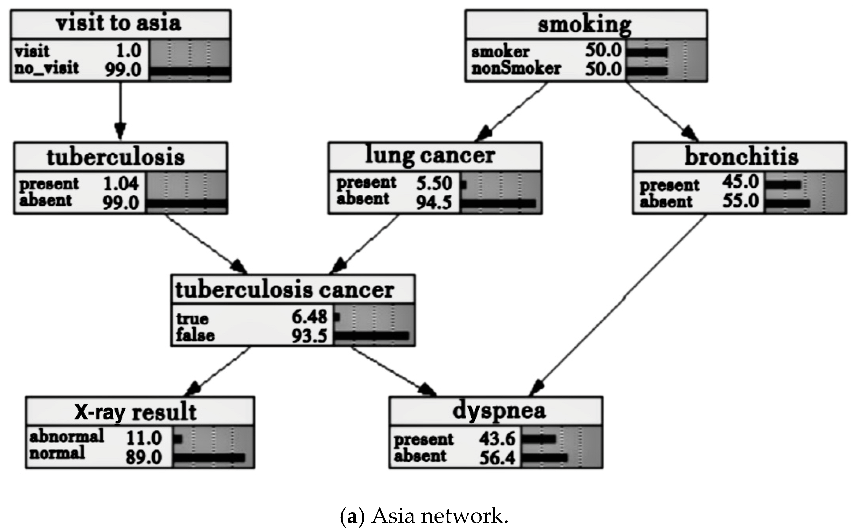
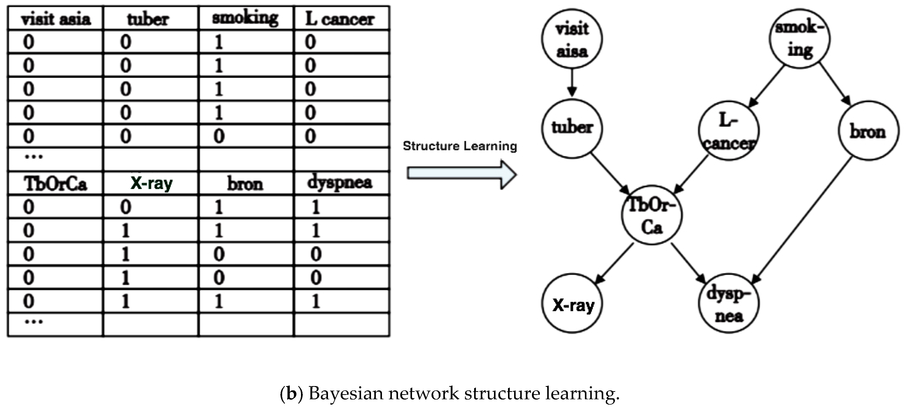
Figure 2.
Directed acyclic graph (DAG) diagram is transformed into adjacent matrix.
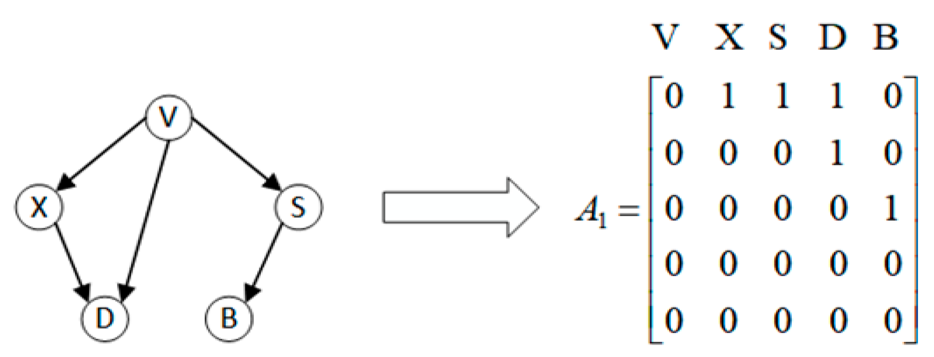
Figure 3.
Ring structure diagram.
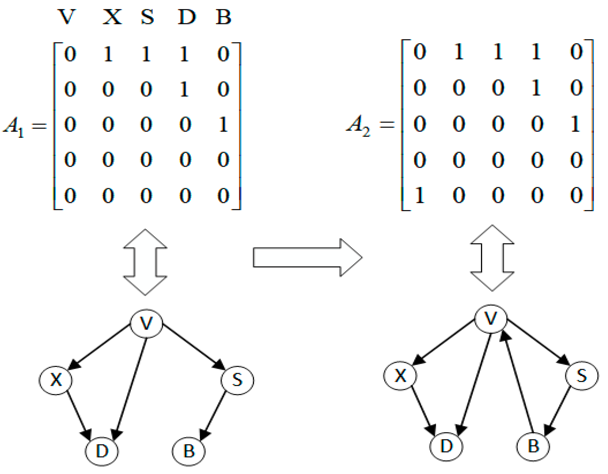
Figure 4.
Standard ASIA.
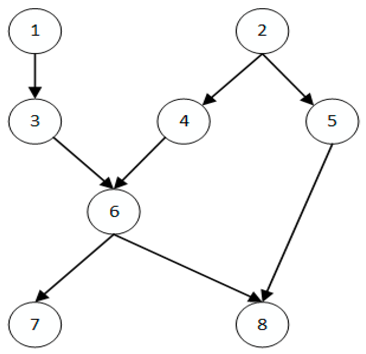
Figure 5.
ASIA after learning.
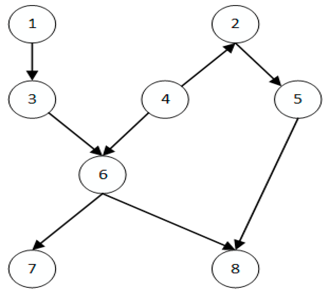
Figure 6.
Standard ALARM.
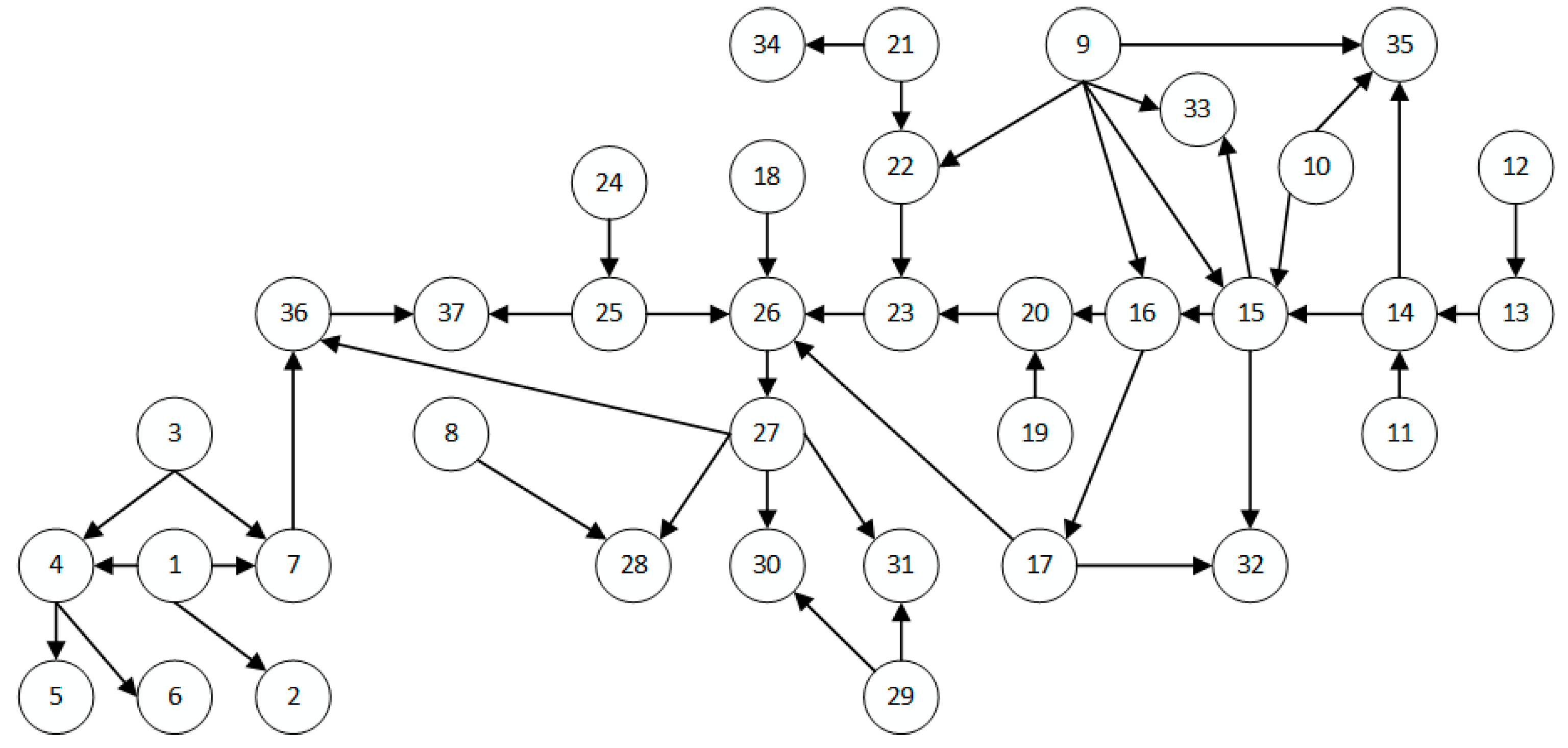
Figure 7.
ALARM after learning.
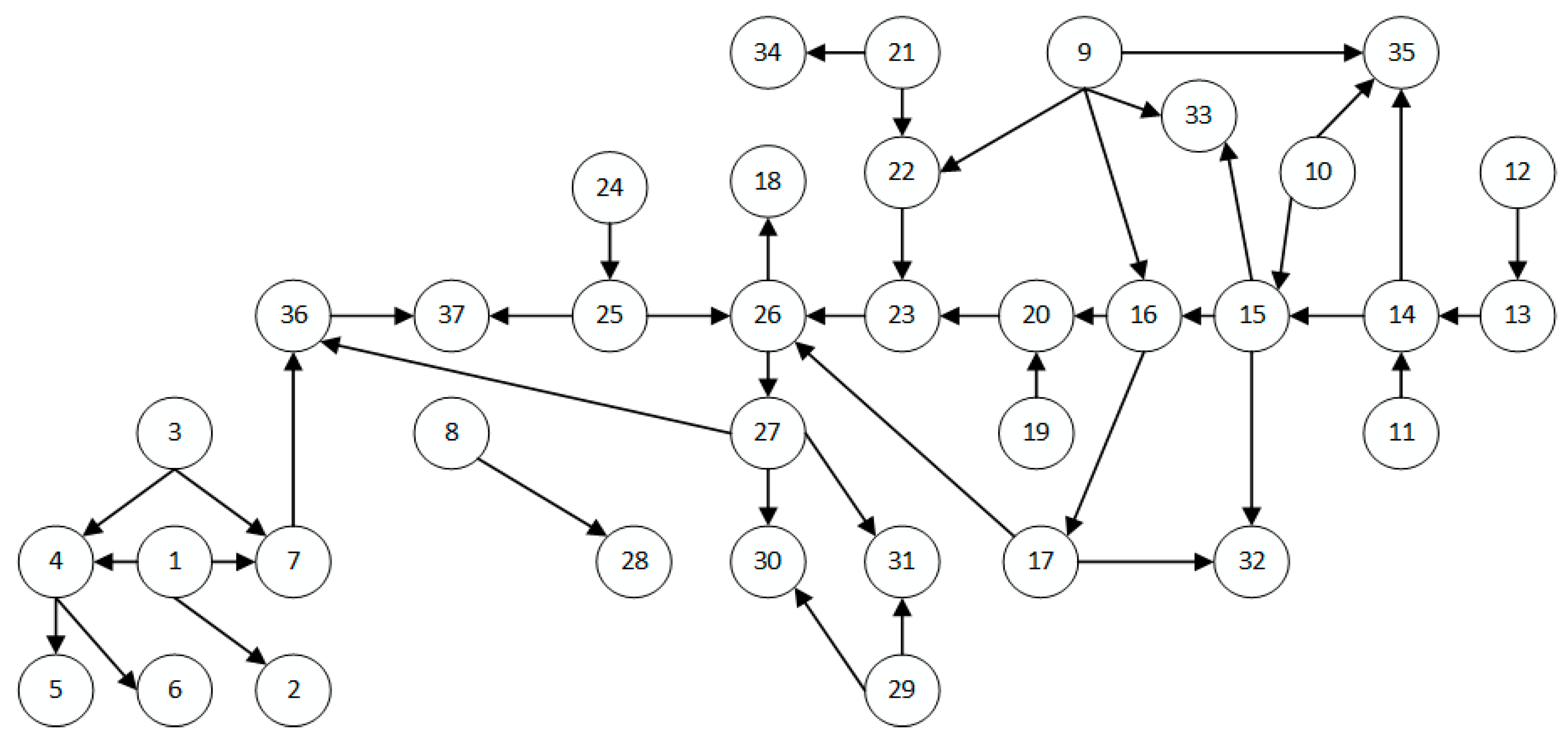
Figure 8.
ASIA experiment results under 1000 data sets.
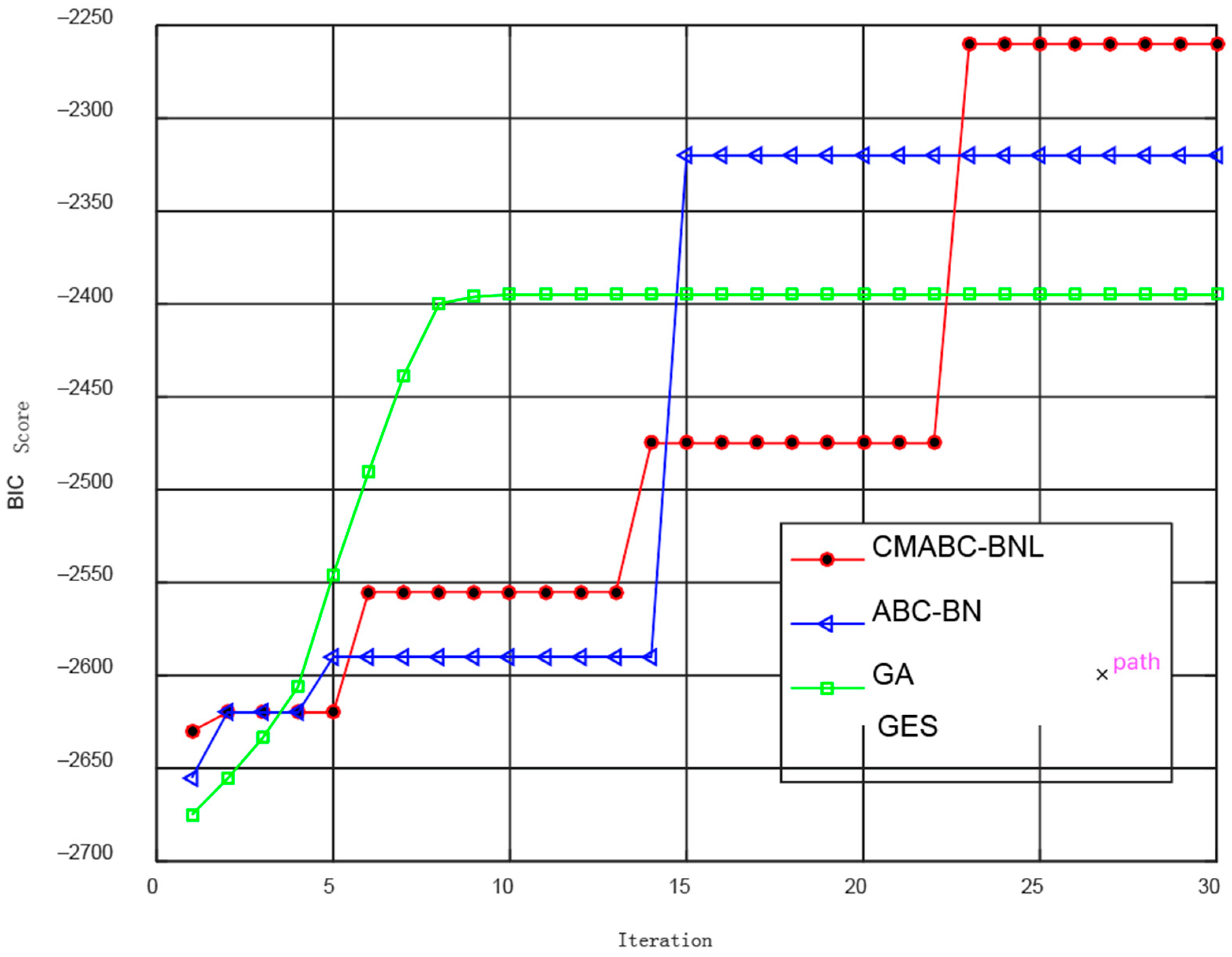
Figure 9.
ALARM experiment results under 5000 data sets.
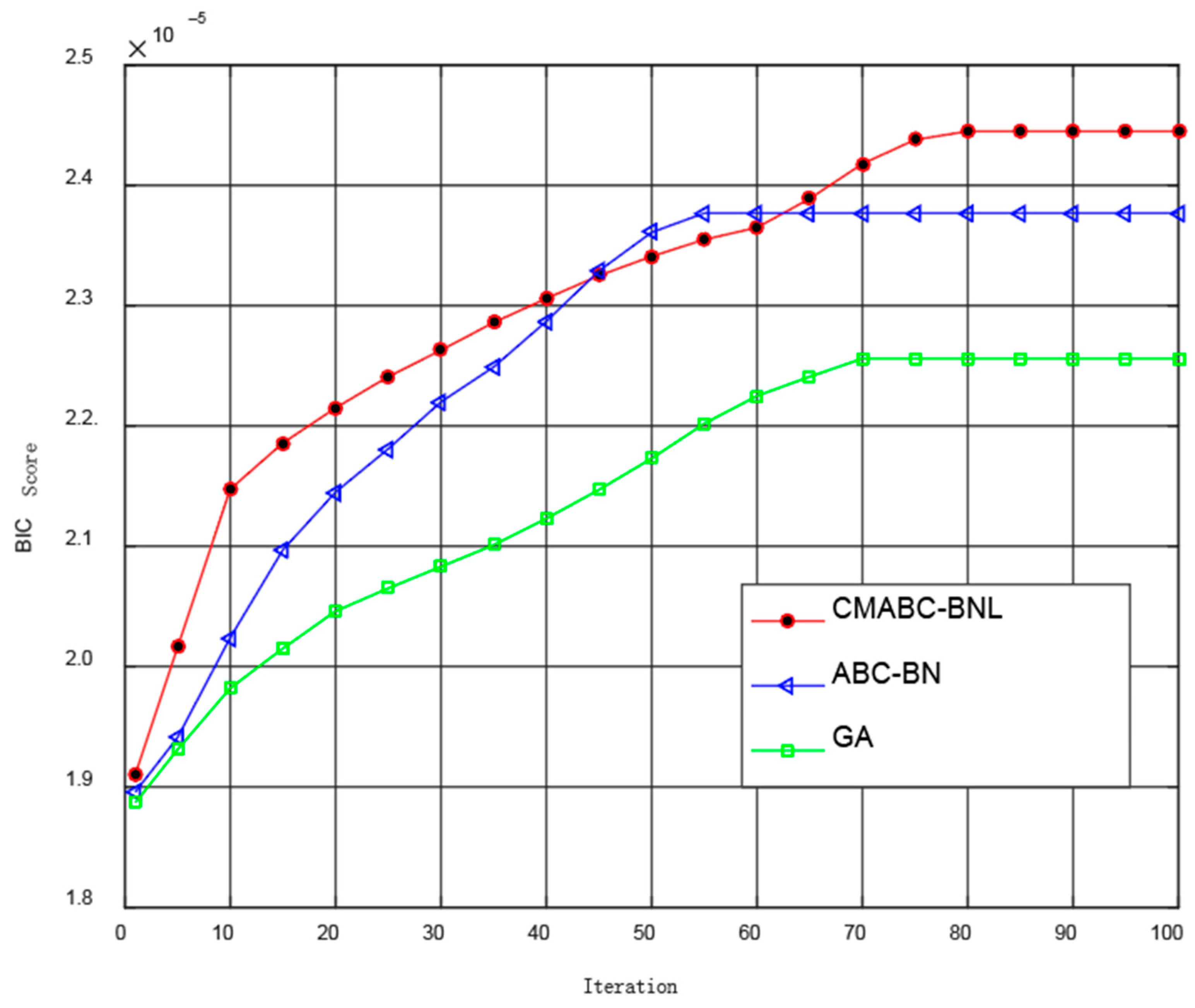
Figure 10.
INSURANCE experiment results under 5000 data sets.

Table 1.
Artificial bee colony optimization and structure learning.
| Bee Colony Searching for Food Source | Bayesian Network Structure Learning |
|---|---|
| Food source | Bayesian network structure |
| Food source quality | Bayesian network structure score |
| Optimal food source | Optimal Bayesian network structure |
Table 2.
Three Bayesian networks.
| Bayesian Network | Nodes | Directed Edges |
|---|---|---|
| ASIA | 8 | 8 |
| ALARM | 37 | 46 |
| INSURANCE | 27 | 52 |
Table 3.
Bayesian network structure learning method based on discrete multi-group artificial bee colony algorithm based on cuckoo algorithm (CMABC-BNL) experimental results.
Table 3.
Bayesian network structure learning method based on discrete multi-group artificial bee colony algorithm based on cuckoo algorithm (CMABC-BNL) experimental results.
| Bayesian Network | Samples | Objective Function Value | Hamming Distance (SHD) | Average Execution Time (Ext) (s) |
|---|---|---|---|---|
| ASIA | 500 | 8.36 × 10⁻⁴ | 0.9 | 2.96 |
| 1000 | 4.42 × 10⁻⁴ | 0.4 | 4.05 | |
| 2000 | 2.18 × 10⁻⁴ | 0.1 | 4.75 | |
| 5000 | 9.01 × 10⁻⁵ | 0 | 6.03 | |
| ALARM | 500 | 1.44 × 10⁻⁴ | 13.8 | 2.54 × 10² |
| 1000 | 8.07 × 10⁻⁵ | 7.5 | 3.85 × 10² | |
| 2000 | 4.27 × 10⁻⁵ | 5.6 | 4.61 × 10² | |
| 5000 | 1.75 × 10⁻⁵ | 3.4 | 7.12 × 10² | |
| INSURANCE | 500 | 1.55 × 10⁻⁴ | 13.2 | 76.7 |
| 1000 | 9.08 × 10⁻⁵ | 10.3 | 1.52 × 10² | |
| 2000 | 6.35 × 10⁻⁵ | 8.4 | 2.43 × 10² | |
| 5000 | 2.17 × 10⁻⁵ | 4.4 | 3.81 × 10² |
Table 4.
Experimental results.
| Training Data | Algorithm | Value | SHD | Ext(s) | F1 Value |
|---|---|---|---|---|---|
| ASIA-1000 | CMABC-BNL | 4.24 × 10⁻⁴ | 0.4 | 5.05 | 0.635 |
| ABC-BN | 4.34 × 10⁻⁴ | 1.5 | 4.27 | 0.616 | |
| GA | 4.17 × 10⁻⁴ | 2.4 | 6.58 | 0.624 | |
| GES | 4.35 × 10⁻⁴ | 2.6 | 0.9 | 0.627 | |
| BNC-PSO | 4.26 × 10⁻⁴ | 1.1 | 3.6 | 0.638 | |
| ASIA-5000 | CMABC-BNL | 9.01 × 10⁻⁵ | 0 | 6.03 | 0.687 |
| ABC-BN | 9.01 × 10⁻⁵ | 0 | 4.34 | 0.646 | |
| GA | 9.01 × 10⁻⁵ | 0 | 8.9 | 0.655 | |
| GES | 9.01 × 10⁻⁵ | 0 | 1.3 | 0.663 | |
| BNC-PSO | 9.01 × 10⁻⁵ | 0 | 4.8 | 0.692 | |
| ALARM-1000 | CMABC-BNL | 8.07 × 10⁻⁵ | 7.5 | 3.85 × 10² | 0.645 |
| ABC-BN | 7.83 × 10⁻⁵ | 8.7 | 3.13 × 10² | 0.621 | |
| GA | 7.45 × 10⁻⁵ | 11.6 | 5.41 × 10² | 0.627 | |
| GES | 8.22 × 10⁻⁵ | 12.3 | 1.47 × 10² | 0.635 | |
| BNC-PSO | 8.14 × 10⁻⁵ | 7.9 | 4.06 × 10² | 0.640 | |
| ALARM-5000 | CMABC-BNL | 1.71 × 10⁻⁵ | 3.4 | 7.12 × 10² | 0.696 |
| ABC-BN | 1.69 × 10⁻⁵ | 4.8 | 6.04 × 10² | 0.658 | |
| GA | 1.63 × 10⁻⁵ | 6.1 | 1.20 × 10³ | 0.669 | |
| GES | 1.83 × 10⁻⁵ | 6.9 | 2.24 × 10² | 0.675 | |
| BNC-PSO | 1.79 × 10⁻⁵ | 4 | 6.92 × 10² | 0.690 | |
| INSURANCE-1000 | CMABC-BNL | 8.73 × 10⁻⁵ | 8.1 | 2.08 × 10² | 0.633 |
| ABC-BN | 8.56 × 10⁻⁵ | 9.2 | 1.97 × 10² | 0.614 | |
| GA | 8.33 × 10⁻⁵ | 10.7 | 3.40 × 10² | 0.618 | |
| GES | 8.54 × 10⁻⁵ | 12.2 | 1.02 × 10² | 0.625 | |
| BNC-PSO | 8.62 × 10⁻⁵ | 8.6 | 1.67 × 10² | 0.632 | |
| INSURANCE-5000 | CMABC-BNL | 2.67 × 10⁻⁵ | 4.3 | 3.80 × 10² | 0.689 |
| ABC-BN | 2.62 × 10⁻⁵ | 5.7 | 3.77 × 10² | 0.647 | |
| GA | 2.50 × 10⁻⁵ | 7.2 | 6.48 × 10² | 0.654 | |
| GES | 2.47 × 10⁻⁵ | 8.9 | 1.31 × 10² | 0.675 | |
| BNC-PSO | 2.35 × 10⁻⁵ | 5 | 3.54 × 10² | 0.683 |
© 2019 by the authors. Licensee MDPI, Basel, Switzerland. This article is an open access article distributed under the terms and conditions of the Creative Commons Attribution (CC BY) license (http://creativecommons.org/licenses/by/4.0/).
Share and Cite
MDPI and ACS Style
Sun, X.; Chen, C.; Wang, L.; Kang, H.; Shen, Y.; Chen, Q. Hybrid Optimization Algorithm for Bayesian Network Structure Learning. Information 2019, 10, 294. https://doi.org/10.3390/info10100294
AMA Style
Sun X, Chen C, Wang L, Kang H, Shen Y, Chen Q. Hybrid Optimization Algorithm for Bayesian Network Structure Learning. Information. 2019; 10(10):294. https://doi.org/10.3390/info10100294
Chicago/Turabian StyleSun, Xingping, Chang Chen, Lu Wang, Hongwei Kang, Yong Shen, and Qingyi Chen. 2019. "Hybrid Optimization Algorithm for Bayesian Network Structure Learning" Information 10, no. 10: 294. https://doi.org/10.3390/info10100294
Note that from the first issue of 2016, this journal uses article numbers instead of page numbers. See further details here.