Article

Quantum-Behaved Particle Swarm Optimization with Weighted Mean Personal Best Position and Adaptive Local Attractor

School of Mathematics and Finance, Chuzhou University, Chuzhou 239000, China
Information 2019, 10(1), 22; https://doi.org/10.3390/info10010022
Submission received: 26 October 2018 / Revised: 19 December 2018 / Accepted: 4 January 2019 / Published: 10 January 2019

Abstract

:
Motivated by concepts in quantum mechanics and particle swarm optimization (PSO), quantum-behaved particle swarm optimization (QPSO) was proposed as a variant of PSO with better global search ability. In this paper, a QPSO with weighted mean personal best position and adaptive local attractor (ALA-QPSO) is proposed to simultaneously enhance the search performance of QPSO and acquire good global optimal ability. In ALA-QPSO, the weighted mean personal best position is obtained by distinguishing the difference of the effect of the particles with different fitness, and the adaptive local attractor is calculated using the sum of squares of deviations of the particles’ fitness values as the coefficient of the linear combination of the particle best known position and the entire swarm’s best known position. The proposed ALA-QPSO algorithm is tested on twelve benchmark functions, and compared with the basic Artificial Bee Colony and the other four QPSO variants. Experimental results show that ALA-QPSO performs better than those compared method in all of the benchmark functions in terms of better global search capability and faster convergence rate.

1. Introduction

Particle swarm optimization (PSO) is a stochastic population-based algorithm proposed by Kennedy and Eberhart [1], which is motivated by the intelligent collective behavior of some animals such as flocks of birds or schools of fish. In PSO, each particle is regarded as a potential solution. All particles have fitness values and velocities, and they fly in a multidimensional search space by learning from the historical information, which contains their memories of the personal best positions and knowledge of the global best position in the groups during the search process. PSO can be easily implemented and is computationally inexpensive, and has few parameters to adjust. For its superiority, PSO has rapidly developed with applications in solving real-world optimization problems in recent years [2,3]. However, PSO is easily trapped into the local optima, and premature convergence appears when it is applied to complex multimodal problems [4]. Many attempts have been made to improve the performance of the PSO [5]. Inspired by quantum mechanics and trajectory analysis of PSO [6], Sun et al. [7,8] proposed a variant of PSO, which is named quantum-behaved PSO (QPSO). Unlike PSO, QPSO needs no velocity vectors for particles, and also has fewer parameters to adjust, making it easier to implement. Since QPSO was proposed, it has attracted much attention and different variants of QPSO have been proposed to enhance the performance from different aspects and successfully applied to solve a wide range of continuous optimization problems [9,10,11,12,13,14]. In general, most current QPSO variants can be classified into three categories [15]: the improvement based on operators from other evolutionary algorithms, hybrid search methods, and cooperative methods. Though those strategies have improved the performance of QPSO in terms of convergence speed and global optimality, it is rather difficult to improve the global search capability and accelerate the rate of convergence simultaneously. In classic QPSO, both the mean personal best position and the local attractor have a great influence on the performance of the algorithm. On one hand, the former is simply the average on the personal best position of all particles, which ignores the difference of the effect of the particles with different fitness on guiding particles to search global optimal solutions. Thus, it is not conducive to improve the global search ability of QPSO. On the other hand, the local attractor for a particle can be obtained as the weighted sum of its personal and global best positions. It has been found that there are few improvements concentrating on the local attractors in QPSO. A novel quantum-behaved particle swarm optimization with Gaussian distributed local attractor point (GAQPSO) is proposed by Sun et al. [16]. In GAQPSO, the local attractor is subject to Gaussian distribution whose mean value is the original local attractor that is defined in classic QPSO. An enhanced QPSO based on a novel computing way of local attractor (EQPSO) is introduced by Jia et al. [17]. In EQPSO, the local attractor is the weighted sum of particle personal and global best positions, using the function designed by the current and total numbers of iterations as the weight. This calculation method cannot monitor the population diversity in real time. Therefore it is not conducive to improve the global search ability of QPSO either. In general, diversity [18] is an important aspect of population-based optimization methods since it influences their performance, and diversity is closely linked to the tradeoff of exploration–exploitation. High diversity facilitates exploration, which is usually required during the initial iterations of the optimization algorithm. Low diversity is indicative of exploitation of a small area of the search space, desired during the latter part of the optimization process. Monitoring the diversity of QPSO populations to construct local attractors to guide particles optimization, thereby improving the algorithm’s ability to search global optimum and accelerating the algorithm’s convergence rate, this practice is rarely reported. In this paper, in order to balance the global and local searching abilities, we propose a set of weighted coefficients that can distinguish the fitness of particles to calculate the mean personal best position, and a novel way of computing the local attractor, furthermore, a new kind of quantum-behaved particle swarm optimization with weighted mean personal best position and adaptive local attractor is designed for numerical optimization. Experimental results show that our proposed method is effective.
The remainder of the paper is structured as follows. A brief introduction of PSO, two versions of QPSO and population diversity of PSO are presented in Section 2. The proposed QPSO with weighted mean personal best position and adaptive local attractor (ALA-QPSO) is given in Section 3. Section 4 provides the experimental results on benchmark functions. Some concluding remarks are given in Section 5.

2. Background

2.1. Paritcle Swarm Optimization

Particle swarm optimization (PSO) is a stochastic population-based algorithm proposed by Kennedy and Eberhart [1], which is motivated by intelligent collective behavior of some animals such as flocks of birds or schools of fish. The candidate solutions for PSO are called particles. The movements of the particles are guided by their own best known position called p b e s t and the entire swarm’s best known position called g b e s t . The position and velocity of the i - th particle is updated according to (1) and (2).
V i t + 1 = ω V i t + c 1 r 1 ( p b e s t i X i t ) + c 2 r 2 ( g b e s t X i t )
X i t + 1 = X i t + V i t + 1
In (1) and (2), X i t = ( x i 1 t , , x i d t , , x i D t ) and V i t = ( v i 1 t , , v i d t , , v i D t ) are the position and velocity vector of D-dimensional space for particle i at iteration t , respectively. c 1 and c 2 are positive constants which control the influence of p b e s t i and g b e s t in the search process, respectively. r 1 and r 2 are random values between 0 and 1. Inertia weight, ω , which was proposed by Shi and Eberhart [19], plays a significant role in balancing the algorithm’s global and local search ability. The fitness value of each particle’s position is determined by a fitness function. PSO is usually executed by repeatedly computing (1) and (2) until a specified number of iterations have reached or the velocity updates are close to zero during the iterations. The pseudo code for the PSO algorithm can be referred to the description proposed by Tian et al. [4].

2.2. Quantum-Behaved Particle Swarm Optimization

Trajectory analysis by Clerc and Kennedy [6] demonstrated that convergence of PSO may be achieved if each particle converges to its local attractor, L A i t = ( l a i 1 t , , l a i d t , , l a i D t ) , defined as follows,
l a i d t = c 1 r 1 p b e s t i d t + c 2 r 2 g b e s t d t c 1 r 1 + c 2 r 2
or
l a i d t = φ p b e s t i d t + ( 1 φ ) g b e s t d t   ,   φ ~ U ( 0 , 1 )
for 1 d D , where t is the iteration number, φ is a random number uniformly distributed on (0, 1), that is φ ~ U ( 0 , 1 ) , p b e s t i represents the best historical position found by particle i , and g b e s t is the current global best position found by the swarm.
Inspired by quantum mechanics and the trajectory analysis of PSO, two versions of quantum-behaved PSO (QPSO), called QPSO with delta potential well model (QDPSO) [7] and a revised QPSO (RQPSO) [8], were proposed one after another by Sun et al. in 2004.
In QDPSO, the position of particle i at iteration t is updated according to (5) by employing the Monte Carlo method.
x i d t + 1 = { l a i d t + α | l a i d t x i d t | ln ( 1 / u )   , if   r a n d 0.5 l a i d t α | l a i d t x i d t | ln ( 1 / u )   , o t h e r w i s e
wherein, both u and r a n d are random numbers uniformly distributed on (0, 1) and α is a positive real number, named the contraction–expansion coefficient, which can be set as α = 0.5 + 0.5 ( T t ) / T to balance the global and local searching ability of QDPSO, wherein parameter t and T are the current and maximum iteration numbers, respectively.
In RQPSO, a global point, denoted as m b e s t = ( m b e s t 1 , , m b e s t d , , m b e s t D ) and called the mean personal best position, is introduced to enhance the global searching ability of QPSO. The global point corresponding to the t - th iteration is computed by Equation (6).
m b e s t t = 1 S ( i = 1 S p b e s t i 1 t , , i = 1 S p b e s t i d t , , i = 1 S p b e s t i D t )   ,   d = 1 , 2 , , D
wherein, parameter t is the current iteration number and S is the number of particles.
The position of particle i at iteration t in RQPSO is updated as shown Equation (7).
x i d t + 1 = { l a i d t + α | m b e s t d t x i d t | ln ( 1 / u )   , if   r a n d 0.5 l a i d t α | m b e s t d t x i d t | ln ( 1 / u )   , o t h e r w i s e
wherein, α and u have the same meaning as the corresponding parameters in (5), and m b e s t d t is the mean personal best position of the population for the d - th dimension at the t - th iteration.

2.3. Population Diversity

The population diversity of PSO is useful for measuring and dynamically adjusting the algorithm’s ability of best path exploration [18]. Lu et al. [20] proposed a method to measure the population diversity using (8).
σ 2 ( t ) = i = 1 S ( f i ( t ) f a v g ( t ) F ) 2 ,   f a v g ( t ) = 1 S i = 1 S f i ( t )
In (8), σ 2 ( t ) is the sum of squares of deviations of the particles’ fitness values, S stands for the swarm size, f i ( t ) is the fitness of the i - th particle at the t - th iteration, f a v g ( t ) is the average fitness of the swarm at the t - th iteration, and F is the normalized calibration factor to confine σ 2 ( t ) . Lu et al. [20] defined F as (9).
F = { max | f i ( t ) f a v g ( t ) | , i f   max | f i ( t ) f a v g ( t ) | > 1 1 , o t h e r w i s e

3. Quantum-Behaved Particle Swarm Optimization with Weighted Mean Personal Best Position and Adaptive Local Attractor (ALA-QPSO)

3.1. Weighted Mean Personal Best Position

In RQPSO, the mean personal best position of the population (mbest) is tracked by particle i during the searching process of the particle. An equal weight coefficient is used to construct the linear combination of each particle best position, which does not distinguish the difference of the effect of the particles with different fitness on guiding particle i to search global optimal solutions. Some useful information hidden in particles’ personal best positions may be lost, which is not conducive to improve the global search ability of QPSO algorithm. For a minimum optimization problem, the elite are the particles which are corresponding to the minimum objective function value. The smaller the objective function value is, the better the particles’ fitness. In societal settings, the elite contribute more towards qualitative improvements. Such an analogy is drawn into the mean personal best position calculation by assigning larger weights to particles having better fitness and smaller weights to comparatively poorer performing particles. In this paper, a weighted mean personal best position, which is calculated by Equations (10) and (11) accordingly to the feedback of fitness values of the particles, can be obtained for guiding particle i to find global optimal solutions for a minimum optimization problem.
r i ( t ) = { 1 S 1 ( 1 f o b j i ( t ) / k = 1 S f o b j k ( t ) ) ,   i f k = 1 S f o b j k ( t ) 0 1 S ,     others
m p b e s t t = i = 1 S r i ( t ) p b e s t i t = ( i = 1 S r i ( t ) p b e s t i 1 t , , i = 1 S r i ( t ) p b e s t i d t , , i = 1 S r i ( t ) p b e s t i D t )
In (10) and (11), t is the current iteration number, f o b j i ( t ) is the objective function value corresponding to the i - th particle at the t - th iteration, S is the number of particles, and r i ( t ) is the coefficient of the best position of the i - th particle at the t - th iteration and is used to construct the weighted mean personal best position.
From (10), it can be deduced that the sum of r i ( t ) is 1 and r i ( t ) is between 0 and 1 at iteration t . When the sum of the objective function value corresponding to all particles is 0, the coefficient r i ( t ) is 1 / S . Otherwise, the smaller f o b j i ( t ) is, the larger r i ( t ) is. That is to say, when constructing a weighted mean personal best position to guide particles for finding optimal solutions for a minimize optimization problem, the larger a particle fitness is, the more important the particle best position is. Thus, the difference of the effect of the particles with different fitness is distinguished.

3.2. Adaptive Local Attractor

Trajectory analysis in [6] show that each particle in the PSO converges to its local attractor. From Equations (3) or (4), the local attractor combines the particle best known position ( p b e s t i ) and the entire swarm’s best known position ( g b e s t ). So, it is very useful to find an efficient way to combine the good information hidden in these two best known positions.
Generally, in population-based optimization methods, during the early stages of the optimization, it is desirable to encourage the individuals to wander through the entire search space, without gathering around local optima. On the other hand, during the latter stages, it is very important to enhance convergence toward the global optima, to find the optimum solution efficiently. Moreover, diversity is an important aspect of population-based optimization methods since it influences their performance, and diversity is closely linked to the exploration–exploitation tradeoff. High diversity facilitates exploration, which is usually required during the initial iterations of the optimization algorithm. A low diversity is indicative of exploitation of a small area of the search space, desired during the latter part of the optimization process. Furthermore, the experience of each particle have more influence on particles when they update their next position at the beginning of iterations, and the experience of other particles has more influence on particles when they update their next position at the later stage of iterations.
Equation (8) shows that σ 2 ( t ) belongs to the interval between 0 and S. When all particles locate in the same position, σ 2 ( t ) is zero. That stands for the swarm aggregation degree at its strongest. Contrarily, σ 2 ( t ) is S on the condition that all absolute differences between the current fitness of all particles and their average fitness equal to one. Thus, the sum of squares of deviations of the particles’ fitness values generally shows a decreasing trend with the number of iterations increasing.
Considering those concerns, in this paper, we propose a novel way of computing the local attractor to achieve the above scheme, and its equation is shown as Equation (12). The objective of this development is to enhance the global search in the early part of the optimization and to encourage the particles to converge toward the global optima at the end of the search. Then, the position of particle i at iteration t is updated as shown (13) in our proposed QPSO with weighted mean personal best position and Adaptive Local Attractor (ALA-QPSO).
A l a i d t = φ σ 2 ( t ) S p b e s t i d t + ( 1 φ ) ( 1 σ 2 ( t ) S ) g b e s t d t   ,   φ U ( 0 , 1 )   ,   d = 1 , 2 , , D
x i d t + 1 = { A l a i d t + α | m p b e s t d t x i d t | ln ( 1 / u )   , if   r a n d 0.5 A l a i d t α | m p b e s t d t x i d t | ln ( 1 / u )   , o t h e r w i s e
In (12), σ 2 ( t ) is the sum of squares of deviations of the particles’ fitness values at iteration t , S is the swarm size, and φ is a random number uniformly distributed on (0, 1). In (13), α and u have the same meaning as the corresponding parameters in (5), m p b e s t d t is the weighted mean personal best position for the d - th dimension at iteration t , and its calculation equation is shown as (11); A l a i d t is the adaptive local attractor of particle i for the d - th dimension at iteration t .

3.3. Quantum-Behaved Particle Swarm Optimization with Adaptive Local Attractor (ALA-QPSO)

Appling the weighted mean personal best position in (11) and the adaptive local attractor in (12) to QPSO, the proposed QPSO with weighted mean personal best position and Adaptive Local Attractor (ALA-QPSO) is described in Algorithm 1 below.
Algorithm 1 ALA-QPSO
  • Initialize the parameters including swarm size S, maximum iteration count T.
  • Initialize particles in the population with random position vectors.
  • Calculate pbest for each particle and gbest for the swarm.
  • Calculate population diversity σ2(t) using (8).
  • Update the weighted mean personal best position mpbestt using (11).
  • Update the adaptive local attractor for each particle using (12).
  • Update the position for each particle using (13).
  • If terminating condition is not meet, go to step 3.

4. Experiments and Discussion

4.1. Benchmark Functions

In this section, twelve classical benchmark functions are listed in Table 1, which are used to verify the performance of the ALA-QPSO algorithm. These benchmark functions are widely adopted in numerical optimization methods [21]. In this paper, the twelve benchmark functions are divided into three groups. The first group includes five unimodal functions ( f 1 ~ f 5 ). The second group includes four complex multimodal functions( f 6 ~ f 9 ), where f 7 owns a large number of local optima so that it is difficult to find the global optimization values, f 8 has many minor local optima, f 9 includes linkage components among variables so it is difficult to reach theoretical optimal values. The third group includes three rotated multimodal functions ( f 10 ~ f 12 ). In Table 1, D denotes the solution space dimension, the global optimal solution ( x * ) and the global optimal value ( f ( x * ) ) of twelve classical benchmark functions are given in column 5 and column 6, respectively.

4.2. Experimental Settings

The benchmark functions defined in the previous subsection are used to test the performance of ALA-QPSO. Five algorithms are used to compare for benchmark functions: Artificial bee colony (ABC) [22], revised QPSO (RQPSO) [8], QPSO with Gaussian distributed attractor (GAQPSO) [16], an enhanced QPSO based on a novel computing way of local attractor (EQPSO) [17], and an improved QPSO with weighted mean best position (WQPSO) [23].
For all compared algorithms, the population size is set to 20 [22,24]. For ABC, the limit number of iterations which a food source cannot be improved (Trial limit) is set to 100 [25]. For all kinds of QPSO, the contraction–expansion coefficient ( α ) decreases linearly from 1.0 to 0.5 during the search process, the local attractors are calculated by Equation (4) except for ALA-QPSO.
Two group experiments are tested. Firstly, setting the convergence criterion as reaching the maximum number of iterations, the mean (Mean) and the standard deviation (SD) of the final fitness value at the end of iteration over multiple runs are compared to test the difference of these compared algorithms solution accuracy and stability. Secondly, setting the convergence criterion as not exceeding the maximum number of iterations and the value of the objective function reaching the allowable precision, the success rate (SR), average convergence iteration number (AIN), and average computational time (Time) over multiple runs are compared for testing the difference of these compared algorithms convergence speed. To obtain an unbiased CPU time comparison, all experiments are conducted using MATLAB R2018a on a personal computer with an Intel Core i7-7500U 2.7 GHz CPU and 16 GB memory.

4.3. Results and Discussions

4.3.1. Comparison of the Solution Accuracy and Stability

In the experiments, the first comparison of tested functions in Table 1 is conducted on 30, 50, and 100 dimensions, and the maximum iteration number ( T ) is set 10,000, 10,000, and 2000, respectively. All compared algorithms terminate calculation when the maximum iteration number is reached. The results are shown in Table 2, Table 3 and Table 4 in terms of the mean and standard deviation of the solutions obtained in the 30 independent runs by each algorithm. Note that the mean of solutions indicates the solution quality of the algorithms, and the standard deviation represents the stability of the algorithms.
Table 2 shows the results on 30 dimension problems. According to the results, ALA-QPSO can find better average objective function values than those of other algorithms on f 6 and f 8 , both ALA-QPSO and EQPSO can find the global optimum on the remaining functions. On the other hand, the standard deviations of the ALA-QPSO algorithm are smaller than those of ABC, GAQPSO, RQPSO, and WQPSO algorithms on all tested functions. Although the standard deviation of ALA-QPSO is larger than that of EQPSO on f 6 and f 8 , the ALA-QPSO algorithm provides smaller average objective function values than those of EQPSO on these two functions.
Table 3 shows that the results on 50 dimension problems. From Table 3, it can be got that both ALA-QPSO and EQPSO can find the global optimum on f 1 ~ f 3 , f 5 , f 7 and f 9 ~ f 12 , and can find equal average objective function value on f 8 . ALA-QPSO obtains better average objective function values than other algorithms on the remaining functions. The standard deviation of ALA-QPSO is less than or equal to that of EQPSO on all the test functions. ALA-QPSO and EQPSO achieve higher accuracy and stronger stability than other algorithms on all test functions.
Table 4 shows that the results on 100 dimension problems. From Table 4, one can see that both
ALA-QPSO and EQPSO provide a solution to the true optimum values for six out of the twelve benchmark functions ( f 5 , f 7 and f 9 ~ f 12 ). ALA-QPSO can find better average objective function values than those of other algorithms on f 1 ~ f 4 and f 6 . Overall, the standard deviation of ALA-QPSO and EQPSO is smaller than that of other algorithms.
To present the total comparison on performance between ALA-QPSO and other algorithms, Table 5 shows the detailed results from the non-parametric Friedman test [26,27]. The last column in this table denotes the corresponding measured p-values, which suggest the significant differences between the compared algorithms at the 0.05 significance level. From Table 5, it can be obtained that there is a significant difference of accuracy and stability among the compared algorithms. Since the Friedman test assigns the lowest rank to the best performing algorithm, the conclusion can be obtained that the ALA-QPSO algorithm has the highest precision and the strongest stability among the compared algorithms.
Moreover, Figure 1 and Figure 2 present the converging curves for the twelve selected functions. Note that the logarithmic of the mean of the best object value according to the t - th iteration, which is denoted log ( y ( t ) ) , is as y -coordinate and the iteration number is as x -coordinate. Since the logarithmic function is a negative infinity (not shown in the figures) when the obtained best object value is zero, some curves stop after a certain number of function evaluations. From Figure 1 and Figure 2, it can be obtained that both ALA-QPSO and EQPSO can find the global optimum of f 1 ~ f 5 , f 7 and f 9 ~ f 12 for 30 dimension problems, also, ALA-QPSO requires fewer iterations than EQPSO; ALA-QPSO can find smaller average objective function values than those of other algorithms on f 6 and f 8 for 30 dimension problems. The convergence curves of ALA-QPSO for all the functions sharply dropped off at a certain point during the early stage of optimization.

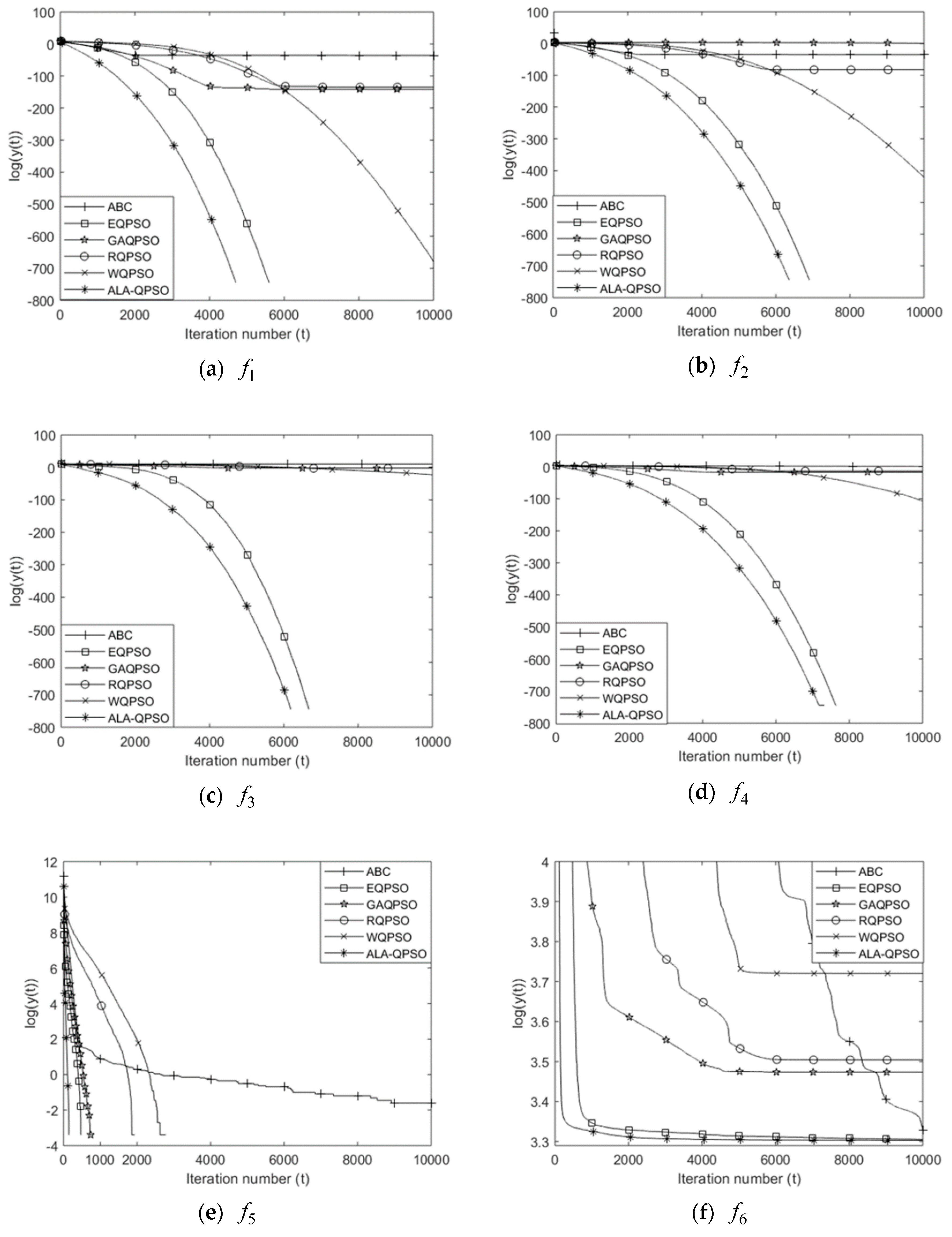
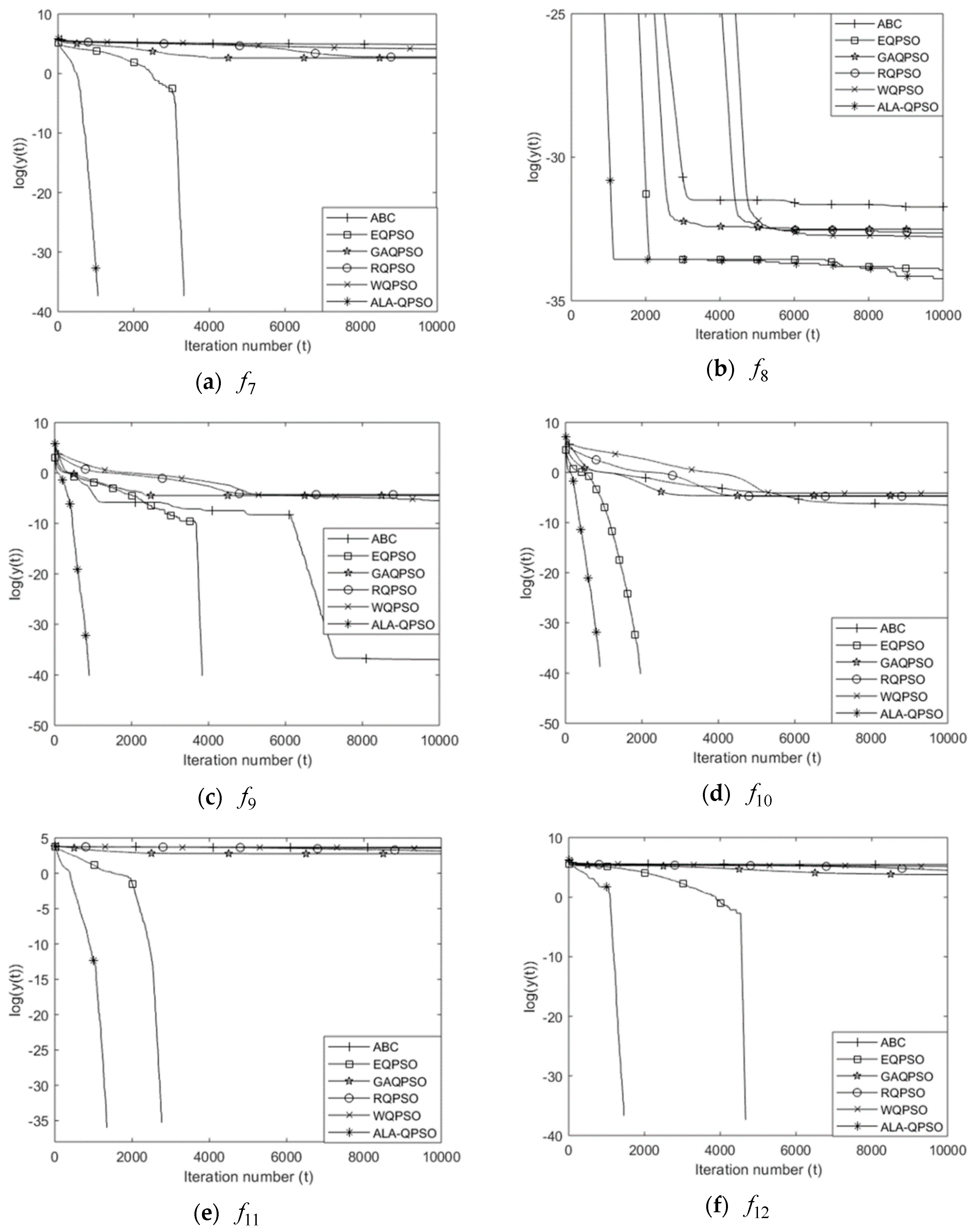
4.3.2. Comparison of the Convergence Speed and Reliability

Each algorithm stops when the maximum number of iterations is arrived at or the value of the objective function is less than or equal to its target accuracy threshold. Wherein, the accuracy threshold for f 6 and f 8 is set as 2.8 × 101 and 5.0 × 10⁻¹⁵, respectively, and for the others is set as 1.0 × 10−50, the maximum iteration number is set as 10,000. Each algorithm was executed 30 times. Three comparing indexes are calculated for the twelve functions with 30 dimensions and are reported in Table 6, Table 7 and Table 8, including the success rate (SR), which is the percentage of the running number of experiments with the final population best solution meeting the accuracy threshold; the average convergence iteration number (AIN), which is the average number of iterations when the algorithm reaches the termination condition over multiple runs; and the average computational time (Time), which is the average of the running time that the algorithm meets the termination condition established for this comparison over multiple runs. Note that some of the compared algorithms may converge to the threshold for the tested functions, while the other may not. The minimum number of iterations required for the objective function meeting an accuracy threshold is used to calculate the AIN, while not meeting; the maximum number of iterations is used for the calculation.
Table 6 presents the success rate of the six compared algorithms on the tested functions with 30-Dimension. Both ALA-QPSO and EQPSO can obtain 100% success rate on all tested functions. The success rate of the two algorithms is higher than those of other algorithms for ten out of the twelve benchmark functions. The results indicate that ALA-QPSO and EQPSO show the best reliability among all the compared algorithms.
Table 7 presents the average convergence iteration numbers of all the compared algorithms on the tested functions with 30-Dimension. The average convergence iteration number of ALA-QPSO is the minimum among those of six compared algorithms for all tested functions. The results show that ALA-QPSO needs the minimum number of convergence iteration to reach the accuracy threshold and that the optimize speed of ALA-QPSO is faster than those of other compared algorithms for all the tested functions.
Table 8 presents the computational time of the six compared algorithms. It can be observed that the computational time of ALA-QPSO is the minimum among those compared algorithms. Since both ALA-QPSO and EQPSO can converge to the threshold for all tested functions, the computational time demonstrates the superiority of the proposed algorithm to some extent.
To present the total comparison on convergence speed and reliability between ALA-QPSO and other algorithms, Table 9 shows the detailed results from the Friedman test. From Table 9, it can be obtained that there is a significant difference of convergence speed and reliability among those compared algorithms. Since the Friedman test assigns the lowest rank to the best performing algorithm, the conclusion can be obtained that the ALA-QPSO algorithm has the fastest convergence speed and the best reliability among all compared algorithms.

5. Conclusions

In this paper, a variant of QPSO, namely ALA-QPSO, is proposed to simultaneously enhance the search performance of QPSO and acquire good global optimal ability. Firstly, a weight parameter is introduced to distinguish the difference of the effect of the particles with different fitness, and is used to obtain the weighted mean personal best position of the population. Secondly, a linear combination of the particle best known position and the entire swarm’s best known position is designed to form the adaptive local attractor by using the sum of squares of deviations of the particles’ fitness values as the linear combination coefficient. The objective of this development is to enhance the global search in the early part of the optimization and to encourage the particles to converge toward the global optima at the end of the search. Finally, the proposed ALA-QPSO algorithm was tested on twelve benchmark functions, and compared with the basic Artificial Bee Colony and the other four QPSO variants. Experimental results show that ALA-QPSO performs better than the compared methods in all of the benchmark functions in terms of better global search capability and faster convergence rate. We conclude that distinguishing the fitness of particles to calculate the weighted mean personal best position and monitoring the diversity of QPSO population to construct adaptive local attractor to guide particles optimization, is feasible. Although the proposed ALA-QPSO exhibited superior performance in the experimental results reported in the previous subsections, it is applicable only to the unconstrained problems in continuous search space. More modifications need to be done to further extend the applicability of the proposed ALA-QPSO to a more general class of optimization problems, including discrete, multi-objective, constrained, as well as dynamic optimization problems. Our further work will focus on using some other strategies to construct more effective local attractor for the QPSO algorithm and applying ALA-QPSO to the real-world optimization problems.

Funding

This research and the APC were funded by the Natural Science Research of the Education Department of Anhui Province, China (Grant no. KJ2016A522).

Acknowledgments

The authors would like to thank the editor and reviewers for their helpful suggestions and valuable comments on a previous version of the present paper.

Conflicts of Interest

The author declares no conflict of interest.

References

  1. Kennedy, J.; Eberhart, R. Particle swarm optimization. In Proceedings of the 1995 IEEE International Conference on Neural Networks, Nagoya, Japan, 4–6 October 1995; pp. 1942–1948. [Google Scholar] [CrossRef]
  2. Zhang, Y.D.; Wang, S.H.; Ji, G.L. A comprehensive survey on particle swarm optimization algorithm and its applications. Math. Probl. Eng. 2015, 2015, 38. [Google Scholar] [CrossRef]
  3. Zhang, Y.D.; Wang, S.H.; Sui, Y.X.; Yang, M.; Liu, B.; Cheng, H.; Sun, J.D.; Jia, W.J.; Phillips, P.; Gorriz, J. Multivariate approach for Alzheimer’s disease detection using stationary wavelet entropy and predator-prey particle swarm optimization. J. Alzheimers Dis. 2018, 65, 855–869. [Google Scholar] [CrossRef] [PubMed]
  4. Tian, D.P.; Shi, Z.Z. MPSO: Modified particle swarm optimization and its applications. Swarm Evol. Comput. 2018, 41, 49–68. [Google Scholar] [CrossRef]
  5. Nickabadi, A.; Ebadzadeh, M.M.; Safabakhsh, R. A novel particle swarm optimization algorithm with adaptive inertia weight. Appl. Soft Comput. 2011, 11, 3658–3670. [Google Scholar] [CrossRef]
  6. Clerc, M.; Kennedy, J. The particle swarm-explosion, stability, and convergence in a multidimensional complex space. IEEE Trans. Evolut. Comput. 2002, 6, 58–73. [Google Scholar] [CrossRef]
  7. Sun, J.; Xu, W.B.; Feng, B. A global search strategy of quantum-behaved particle swarm optimization. In Proceedings of the 2004 IEEE Conference on Cybernetics and Intelligent Systems, Singapore, 1–3 December 2004; pp. 111–116. [Google Scholar]
  8. Sun, J.; Feng, B.; Xu, W.B. Particle swam optimization with particles having quantum behavior. In Proceedings of the 2004 IEEE Congress on Evolutionary Computation, Portland, OR, USA, 19–23 June 2004; pp. 326–331. [Google Scholar]
  9. Zhang, Y.D.; Ji, G.L.; Yang, J.Q.; Wang, S.H.; Dong, Z.C. Preliminary research on abnormal brain detection by wavelet-energy and quantum-behaved PSO. Biomed. Eng. 2016, 61, 431–441. [Google Scholar] [CrossRef]
  10. Li, L.L.; Jiao, L.C.; Zhao, J.Q.; Shang, R.H.; Gong, M.G. Quantum-behaved discrete multi-objective particle swarm optimization for complex network clustering. Pattern Recogn. 2017, 63, 1–14. [Google Scholar] [CrossRef]
  11. Feng, Z.K.; Niu, W.J.; Cheng, C.T. Multi-objective quantum-behaved particle swarm optimization for economic environmental hydrothermal energy system scheduling. Energy 2017, 131, 165–178. [Google Scholar] [CrossRef]
  12. Fang, W.; Sun, J.; Wu, X.; Palade, V. Adaptive web QoS controller based on online system identification using quantum-behaved particle swarm optimization. Soft Comput. 2015, 19, 1715–1725. [Google Scholar] [CrossRef]
  13. Sing, M.R.; Mahapatra, S.S. A quantum behaved particle swarm optimization for flexible job shop scheduling. Comput. Ind. Eng. 2016, 93, 36–44. [Google Scholar] [CrossRef]
  14. Tang, D.; Cai, Y.; Xue, Y. A quantum-behaved particle swarm optimization with memetic algorithm and memory for continuous non-linear large scale problems. Inf. Sci. 2014, 289, 162–189. [Google Scholar] [CrossRef]
  15. Yang, Z.L.; Wu, A.; Min, H.Q. An improved quantum-behaved particle swarm optimization algorithm with elitist breeding for unconstrained optimization. Comput. Intell. Neurosci. 2015, 2015, 12. [Google Scholar] [CrossRef] [PubMed]
  16. Sun, J.; Fang, W.; Palade, V.; Wu, X.J.; Xu, W.B. Quantum-behaved particle swarm optimization with Gaussian distributed local attractor point. Appl. Math. Comput. 2011, 218, 3763–3775. [Google Scholar] [CrossRef]
  17. Jia, P.; Duan, S.; Yan, J. An enhanced quantum-behaved particle swarm optimization based on a novel computing way of local attractor. Information 2015, 6, 633–649. [Google Scholar] [CrossRef]
  18. Han, F.; Liu, Q. A diversity-guided hybrid particle swarm optimization algorithm based on gradient search. Neurocomputing 2014, 137, 234–240. [Google Scholar] [CrossRef]
  19. Shi, Y.; Eberhart, R. A modified particle swarm optimizer. In Proceedings of the 1998 IEEE Congress on Computational Intelligence, Anchorage, AK, USA, 4–9 May 1998; pp. 69–73. [Google Scholar]
  20. Lu, Z.S.; Hou, Z.R.; Du, J. Particle swarm optimization with adaptive mutation. Front. Electr. Electron. Eng. China 2006, 1, 99–104. [Google Scholar] [CrossRef]
  21. Chen, K.; Zhou, F.Y.; Liu, A.L. Chaotic dynamic weight particle swarm optimization for numerical function optimization. Knowl-Based Syst. 2018, 139, 23–40. [Google Scholar] [CrossRef]
  22. Karaboga, D.; Akay, B. A modified Artificial Bee Colony algorithm for real-parameter optimization. Inf. Sci. 2012, 192, 120–142. [Google Scholar]
  23. Xi, M.L.; Sun, J.; Xu, W.B. An improved quantum-behaved particle swarm optimization algorithm with weighted mean best position. Appl. Math. Comput. 2008, 205, 751–759. [Google Scholar] [CrossRef]
  24. Zhang, L.P.; Yu, H.J.; Hu, S.X. Optimal choice of parameters for particle swarm optimization. J. Zhejiang Univ. Sci. 2005, 6, 528–534. [Google Scholar]
  25. Ye, W.X.; Feng, W.Y.; Fan, S.H. A novel multi-swarm particle swarm optimization with dynamic learning strategy. Appl. Soft Comput. 2017, 61, 832–843. [Google Scholar] [CrossRef]
  26. Derrac, J.; García, S.; Molina, D.; Herrera, F. A practical tutorial on the use of nonparametric statistical tests as a methodology for comparing evolutionary and swarm intelligence algorithms. Swarm Evol. Comput. 2011, 1, 3–18. [Google Scholar] [CrossRef]
  27. Friedman, M. The use of ranks to avoid the assumption of normality implicit in the analysis of variance. J. Am. Stat. Assoc. 1937, 32, 675–701. [Google Scholar] [CrossRef]
Figure 1. Convergence graphs of six algorithms on 30-D benchmark functions. f 1 ~ f 6 : y ( t ) represents the mean of the best object value according to the t - th .
Information 10 00022 g001
Figure 2. Convergence graphs of six algorithms on 30-D benchmark functions. f 7 ~ f 12 : y ( t ) represents the mean of the best object value according to the t - th .
Information 10 00022 g002
Table 1. High dimensional classical benchmark functions.
GroupNameTest Function 1Search Space Global opt. x * f ( x * )
UnimodalSphere f 1 ( x ) = i = 1 D x i 2 [ 100 , 100 ] D [ 0 ] D 0
Schwefel’s 2.22 f 2 ( x ) = i = 1 D | x i | + i = 1 D | x i | [ 10 , 10 ] D [ 0 ] D 0
Schwefel’s 1.2 f 3 ( x ) = i = 1 D ( j = 1 i x j ) 2 [ 100 , 100 ] D [ 0 ] D 0
Schwefel’s 2.21 f 4 ( x ) = max i { | x i | , 1 i n } [ 100 , 100 ] D [ 0 ] D 0
Step f 5 ( x ) = i = 1 D ( x i + 0.5 ) 2 [ 100 , 100 ] D [ - 0.5 ] D 0
MultimodalRosenbrock f 6 ( x ) = i = 1 D 1 [ 100 ( x i 2 x i + 1 ) 2 + ( x i 1 ) 2 ] [ 30 , 30 ] D [ 1 ] D 0
Rastrigin f 7 ( x ) = i = 1 D ( x i 2 10 cos ( 2 π x i ) + 10 ) [ 5.12 , 5.12 ] D [ 0 ] D 0
Ackley f 8 ( x ) = 20 exp ( 0.2 1 D i = 1 D x i 2 ) exp ( 1 D i = 1 D cos 2 π x i ) + 20 + e [ 32 , 32 ] D [ 0 ] D 0
Griewank f 9 ( x ) = 1 4000 i = 1 D x i 2 i = 1 D cos ( x i i ) + 1 [ 600 , 600 ] D [ 0 ] D 0
RotatedRotated Griewank f 10 ( x ) = 1 4000 i = 1 D y i 2 i = 1 D cos ( y i i ) + 1 , y = M x , M is an orthogonal matrix. [ 600 , 600 ] D [ 0 ] D 0
Rotated Weierstrass f 11 ( x ) = i = 1 D k = 0 20 [ 1 2 k cos ( 3 k ( 2 π y i + π ) ) ] D k = 0 20 [ 1 2 k cos ( 3 k π ) ]   ,   y = M x , M is an orthogonal matrix. [ 0.5 , 0.5 ] D [ 0 ] D 0
Rotated Rastrigin f 12 ( x ) = i = 1 D ( y i 2 10 cos ( 2 π y i ) + 10 ) ,   y = M x , M is an orthogonal matrix. [ 5.12 , 5.12 ] D [ 0 ] D 0
1 The orthogonal rotation matrix M is generated by the Salomon’s method and used to calculate f 10 ~ f 12 .
Table 2. Mean and standard deviations of the function values ( S = 20; D = 30; T = 10,000).
f CriteriaABCEQPSOGAQPSORQPSOWQPSOALA-QPSO
f 1 Mean3.2115 × 10−1604.3697 × 10−623.0586 × 10−591.0489 × 10−2950
SD6.4479 × 10−1702.3700 × 10−619.3210 × 10−5900
f 2 Mean6.5535 × 10−1602.62951.8088 × 10−361.9995 × 10−1830
SD7.4422 × 10−1709.6839 × 10−19.8507 × 10−3600
f 3 Mean2.5595 × 10409.4301 × 10−26.8640 × 10−25.8909 × 10−110
SD3.4939 × 10308.8509 × 10−27.5320 × 10−21.5317 × 10−100
f 4 Mean3.183104.8093 × 10−81.3798 × 10−66.8607 × 10−470
SD2.142106.9539 × 10−82.0440 × 10−63.0515 × 10−460
f 5 Mean2.0000 × 10−100000
SD4.0684 × 10−100000
f 6 Mean2.7875 × 1012.7256 × 1013.2247 × 1013.3247 × 1014.1283 × 1012.7188 × 101
SD2.4684 × 1013.4765 × 10−22.1339 × 1012.2535 × 1013.0141 × 1012.0527 × 10−1
f 7 Mean1.3148 × 10201.3565 × 1011.5995 × 1016.2577 × 1010
SD3.9721 × 10103.72724.16572.8038 × 1010
f 8 Mean1.6520 × 10−141.8356 × 10−157.6383 × 10−156.6909 × 10−155.8620 × 10−151.3619 × 10⁻¹⁵
SD3.2788 × 10−151.5283 × 10−152.8908 × 10−151.8027 × 10−151.0840 × 10−151.7413 × 10⁻¹⁵
f 9 Mean8.5117 × 10−1701.1383 × 10−21.3693 × 10−24.1262 × 10−30
SD8.5915 × 10−1701.6879 × 10−21.4073 × 10−27.9803 × 10−30
f 10 Mean1.4624 × 10−309.8340 × 10−38.7590 × 10−31.6271 × 10⁻²⁰
SD4.1486 × 10−301.5979 × 10−21.5123 × 10−22.3173 × 10⁻²⁰
f 11 Mean3.9661 × 10101.5813 × 1012.2942 × 1013.4979 × 1010
SD1.037703.38347.35314.76940
f 12 Mean2.3683 × 10204.3726 × 1019.0690 × 1011.7675 × 1020
SD1.2881 × 10102.3307 × 1015.9659 × 1011.6948 × 1010
Mean: mean of objective values. SD: standard deviation.
Table 3. Mean and standard deviations of the function values (S = 20; D = 50; T = 10,000).
f CriteriaABCEQPSOGAQPSORQPSOWQPSOALA-QPSO
f 1 Mean3.6199 × 10−406.7392 × 10−296.0020 × 10−231.1225 × 10−1870
SD1.3183 × 10−301.5822 × 10−281.6548 × 10−2200
f 2 Mean2.0161 × 10−1503.2628 × 1011.8119 × 10−151.8498 × 10−1220
SD3.4824 × 10−1603.92166.1161 × 10−154.8665 × 10−1220
f 3 Mean9.4472 × 10402.1336 × 1026.1731 × 1021.0466 × 1020
SD8.6811 × 10306.1093 × 1013.2722 × 1022.0518 × 1020
f 4 Mean6.0318 × 1014.9407 × 10−3242.1843 × 10−22.4619 × 10−12.7663 × 10−190
SD9.139109.5378 × 10−39.7297 × 10−29.2674 × 10−190
f 5 Mean2.2833 × 101003.3333 × 10−200
SD4.5945001.8257 × 10−100
f 6 Mean6.2760 × 1064.7372 × 1015.3485 × 1015.8728 × 1018.3258 × 1014.7255 × 101
SD2.7022 × 1062.5471 × 10−12.1756 × 1012.7264 × 1014.4773 × 1012.1455 × 10−1
f 7 Mean3.9881 × 10203.0224 × 1013.9652 × 1011.9921 × 1020
SD3.3527 × 10109.78231.1177 × 1015.6608 × 1010
f 8 Mean1.6808 × 10−62.6645 × 10−159.9654 × 10−146.0201 × 10−137.1646 × 10−152.6645 × 10⁻¹⁵
SD3.3123 × 10−601.2662 × 10−137.5045 × 10−132.4567 × 10−150
f 9 Mean4.1901 × 10−402.3000 × 10−34.6762 × 10−31.5135 × 10⁻³⁰
SD2.2474 × 10−304.4326 × 10−39.5542 × 10−33.4264 × 10⁻³⁰
f 10 Mean1.399501.9316 × 10−22.1549 × 10−21.4702 × 10−10
SD8.3632 × 10−109.5536 × 10−31.2197 × 10−21.0084 × 10⁻¹⁰
f 11 Mean7.4129 × 10103.4137 × 1015.9507 × 1016.9111 × 1010
SD1.220806.43571.1104 × 1015.83220
f 12 Mean5.3144 × 10201.3132 × 1022.5030 × 1023.7453 × 1020
SD1.9377 × 10105.3289 × 1019.9465 × 1013.1666 × 1010
Mean: mean of objective values. SD: standard deviation.
Table 4. Mean and standard deviations of the function values (S = 20; D = 100; T = 2000).
f CriteriaABCEQPSOGAQPSORQPSOWQPSOALA-QPSO
f 1 Mean5.6282 × 1048.9938 × 10−2701.2873 × 1017.8668 × 1016.8659 × 10−164.9774 × 10−283
SD9.1711 × 10309.30894.2189 × 1011.0448 × 10−150
f 2 Mean2.4596 × 10161.6177 × 10−1503.6510 × 1031.95785.3771 × 10−134.0840 × 10−155
SD8.1969 × 10168.7797 × 10−1501.7832 × 1045.7540 × 10−14.7000 × 10−137.1024 × 10−155
f 3 Mean4.4087 × 1051.6281 × 10−1712.5833 × 1043.9155 × 1047.3538 × 1048.8599 × 10−172
SD4.5889 × 10404.1772 × 1036.8323 × 1031.4797 × 1040
f 4 Mean9.1993 × 1013.6553 × 10−1082.0536 × 1012.9877 × 1011.7931 × 1011.9923 × 10−108
SD1.24798.9262 × 10−1082.59613.44359.79993.7736 × 10−108
f 5 Mean5.2736 × 10407.1800 × 1011.7167 × 10200
SD1.2741 × 10407.1461 × 1011.0108 × 10200
f 6 Mean2.0590 × 1089.8213 × 1012.0340 × 1032.2630 × 1049.7107 × 1019.8063 × 101
SD6.1190 × 1072.4313 × 10−11.0493 × 1032.1261 × 1044.4917 × 10−13.7079 × 10⁻¹
f 7 Mean1.1560 × 10301.5749 × 1022.4022 × 1026.7970 × 1020
SD6.9418 × 10102.8214 × 1014.8421 × 1011.2108 × 1020
f 8 Mean1.7282 × 1012.6645 × 10−151.49152.73222.8350 × 10−92.6645 × 10⁻¹⁵
SD7.5513 × 10−105.3252 × 10−15.0710 × 10−11.8879 × 10−90
f 9 Mean4.6645 × 10201.06901.69274.9550 × 10−30
SD9.1110 × 10101.3023 × 10−13.6188 × 10−11.2937 × 10−20
f 10 Mean2.1488 × 10307.00631.3661 × 1015.0429 × 10−20
SD3.8195 × 10202.68426.15571.3579 × 10−10
f 11 Mean1.6597 × 10206.9628 × 1018.3404 × 1011.2400 × 1020
SD1.882907.58496.33362.7652 × 1010
f 12 Mean1.8132 × 10305.7674 × 1028.8909 × 1029.7741 × 1020
SD6.7997 × 10101.2077 × 1021.5362 × 1025.4787 × 1010
Mean: mean of objective values. SD: standard deviation.
Table 5. Average ranking of algorithms for test functions, as obtained by the Friedman test.
D TCriteriaABCEQPSOGAQPSORQPSOWQPSOALA-QPSOp-Value
3010,000Mean5.171.714.174.334.081.547.02 × 10−8
SD4.831.714.424.503.671.881.18 × 10−6
5010,000Mean5.671.633.714.583.881.543.16 × 10−9
SD5.001.673.965.003.791.583.85 × 10−8
1002000Mean6.001.833.754.583.421.427.45 × 10−10
SD5.251.584.174.673.831.501.70 × 10−8
Table 6. The success rate of six algorithms (S = 20; D = 30; T = 10,000).
SR (%)ABCEQPSOGAQPSORQPSOWQPSOALA-QPSO
f 1 0.0 100.0 100.0 100.0 100.0 100.0
f 2 0.0 100.0 0.0 0.0 100.0 100.0
f 3 0.0 100.0 0.0 0.0 0.0 100.0
f 4 0.0 100.0 0.0 0.0 13.3 100.0
f 5 90.0 100.0 100.0 100.0 100.0 100.0
f 6 83.3 100.0 83.3 83.3 90.0 100.0
f 7 0.0 100.0 0.0 0.0 0.0 100.0
f 8 0.0 100.0 0.0 0.0 10.0 100.0
f 9 26.7 100.0 50.0 46.7 66.7 100.0
f 10 0.0 100.0 0.0 0.0 3.3 100.0
f 11 0.0 100.0 0.0 0.0 0.0 100.0
f 12 0.0 100.0 0.0 0.0 0.0 100.0
Table 7. The average convergence iteration number of six algorithms (S = 20; D = 30; T = 10,000).
AINABCEQPSOGAQPSORQPSOWQPSOALA-QPSO
f 1 1.0000 × 1042.6734 × 1033.5675 × 1035.4186 × 1035.6027 × 1031.6216 × 103
f 2 1.0000 × 1043.3180 × 1031.0000 × 1041.0000 × 1046.4183 × 1032.4406 × 103
f 3 1.0000 × 1043.9438 × 1031.0000 × 1041.0000 × 1041.0000 × 1042.7628 × 103
f 4 1.0000 × 1044.0493 × 1031.0000 × 1041.0000 × 1049.9972 × 1033.0298 × 103
f 5 4.7939 × 1034.0820 × 1025.6233 × 1021.7512 × 1032.3136 × 1031.1700 × 102
f 6 3.9238 × 1031.7044 × 1032.5791 × 1033.7521 × 1034.1808 × 1038.8953 × 102
f 7 1.0000 × 1042.5510 × 1031.0000 × 1041.0000 × 1041.0000 × 1048.5687 × 102
f 8 1.0000 × 1042.0492 × 1031.0000 × 1041.0000 × 1049.9056 × 1031.0859 × 103
f 9 8.7063 × 1032.3023 × 1036.0576 × 1037.3058 × 1037.5273 × 1038.3030 × 102
f 10 1.0000 × 1041.8583 × 1031.0000 × 1041.0000 × 1049.9930 × 1038.4923 × 102
f 11 1.0000 × 1042.3043 × 1031.0000 × 1041.0000 × 1041.0000 × 1041.1307 × 103
f 12 1.0000 × 1043.7039 × 1031.0000 × 1041.0000 × 1041.0000 × 1048.9340 × 102
Table 8. The computational time of six algorithms (S = 20; D = 30; T = 10,000).
Time (S)ABCEQPSOGAQPSORQPSOWQPSOALA-QPSO
f 1 5.3178 1.4530 2.1226 2.6127 4.3395 0.8115
f 2 5.0471 2.7620 8.4172 5.1515 4.0062 1.2683
f 3 7.3963 4.3318 6.1789 6.2239 6.0860 1.8055
f 4 6.3163 3.4015 4.8744 5.0325 4.8261 1.4174
f 5 3.1655 0.3873 0.2949 0.7712 1.0777 0.0748
f 6 2.7310 1.6312 1.3465 1.7113 2.1007 0.4562
f 7 5.2583 2.1870 4.9350 4.5979 4.5153 0.4413
f 8 5.0777 2.0003 4.3977 4.5203 4.8249 0.5535
f 9 3.5959 2.2915 2.7715 3.4466 3.6319 0.4417
f 10 6.1578 2.7307 7.6677 7.0954 7.8027 0.6347
f 11 24.0117 8.4135 23.0703 18.4729 23.8336 2.4332
f 12 7.7361 2.5692 6.4690 6.6778 6.9953 0.6512
Table 9. Average ranking of competitor algorithms for the twelve benchmark functions, as obtained by the Friedman test (S = 20; D = 30; T = 10,000).
CriteriaABCEQPSOGAQPSORQPSOWQPSOALA-QPSOp-Value
Time5.502.173.674.174.501.007.94 × 10−9
AIN5.082.004.174.504.251.006.88 × 10−10
SR5.081.794.424.503.421.793.90 × 10−9

