A. Country Groups
Country groups are identified by the countries with the largest population in the group as of 2010. The following eight groups are chosen to have roughly balanced total energy production and consumption in each group, and to be of comparable long-term limit population. Exceptions are that the limit population of the USA group is noticeably smaller than average, and the limit population of the India group is noticeably larger than average. These eight groups are (1) China: People’s Republic of China, Democratic People’s Republic of Korea, and Mongolia; (2) India: Afghanistan, Bhutan, India, Iran, Maldives, Nepal, Pakistan, and Sri Lanka; (3) Nigeria: Africa south of the Sahel countries that are included with Ethiopia below; (4) Brazil: Western Hemisphere except USA and Canada; (5) Ethiopia-Egypt: Arabian Peninsula, Chad, Djibouti, Egypt, Eritrea, Mali, Mauritania, Niger, Somalia, South Sudan, Sudan, North Africa, Iraq, Israel and the Occupied Territories, Jordan, Lebanon, Syria, Turkey, and Western Sahara; (6) Indonesia: All countries not in other groups, including Pacific islands and the countries in the Association of Southeast Asian Nations; (7) EU: Europe including French overseas island Departments, and the former Soviet Union; and (8) USA: Canada, Guam, Puerto Rico, and U.S. Virgin Islands. In addition, Japan is treated alone as a separate “group” because the 2011 tsunami greatly perturbed its energy mix.
B. Population and GDP
The parameters discussed in this paragraph are in convenient dimensionless units. The relationship between these parameters and their dimensional counterparts is described below. The utility of per capita consumption
C for each country group is taken to be
, with population approximated as proportional to labor,
L, and with
θ a universal constant. Population is approximated as a logistic function of time, calibrated against historical data. Total discounted total future welfare starting at a time
t is proportional to
with social discount rate
ρ a universal constant. Consumption is
. Here the depreciation rate
r is a universal constant,
K is capital stock, and
is the time rate of change of capital stock. GDP is
Y/
α with
where the rate of energy use is
. Overall economic productivity is a logistic function
, with constants
ν and
t1 calibrated against time-series data for each country group.
βk and
βℓ are respectively the fractions of total capital and labor in the energy sector. Welfare is maximized with sustainability as a terminal boundary condition when
K,
k, and
ℓ solve a set of coupled Euler-Lagrange differential equations with regularity as
t → ∞,
i.e., as
z = 1 −
a → 0. The universal constant
ω = 1 −
α is the fraction of GDP paid to labor. Carbon intensity
p is the carbon/energy use ratio divided by that for coal. The universal constant 1/(1 +
h) is the ratio of the energy produced with a given productivity and amounts of capital and labor using carbon-free sources to that using high-carbon sources.
In the above equations, time is universally expressed in units of the “capitalization time”
, where
is the depreciation rate per year and
is the social discount rate per year. For each country group, monetary units
K are expressed in units of that group’s long-term equilibrium limit value of capital stock. All dimensional monetary units are in purchasing power parity (PPP). The energy use rate
w is expressed in units of its long-term limit value for each group. The values of the universal parameters used here are taken from Singer
et al. [
14]. Except for
h = 1.5, these values were calibrated against empirical data. These values are
α = 0.325,
θ = 1.345,
= 0.107/year, and
= 0.218/year, resulting in a “capitalization time”
= 7.76 years. Using the approximation discussed below, the results shown in this paper are independent of the value of the parameter
β. The value used for
h is chosen here as an example roughly compatible with a ratio of
h + 1 = 2.5 in the cost of electricity from non-fossil energy sources and from inexpensive fossil fuels.
The results shown in this paper rely on expansion of the solution of the welfare maximization problem in three parameters. Expanding only to lowest order in the energy fraction of capital, β, allows the evolution of total capital and GDP to be calibrated against time-series data for GDP independently of data on energy and carbon use. The parameter β is a measure of the portion of capital and labor used for procuring energy consumed. That energy can either be produced domestically, imported, or a combination both. Generally that portion is only a few percent, so β is a good expansion parameter.
Expansion is through first order in the capitalization lag parameter δ = νθ/ω. This parameter is a measure of the maximum value of the difference between capital stock and what it would relax to if productivity and labor were frozen, divided by the total capital stock. For some cases, particularly China, we have δ ≈ 1, and the results thus provide only a semi-empirical formula for the period of historical time-series data used to calibrate the a priori uncertain parameters in the model for that group. The term “semi-empirical” here is meant to imply that the capitalization lag phenomenon is accounted for, but not in a manner exactly consistent with the similar but more accurate solutions that we have obtained in exploratory work on the China and USA groups using exact numerical solutions with adjustable parameters calibrated against the same data. That numerical integration requires a shooting method starting from a triple power series expansion in z around the regular singular point z = 0. The nonlinear differential equations to be solved have a movable singular point at larger values of z, i.e., earlier times, and great care in choosing the one adjustable boundary condition parameter has to be exercised to get a solution that does not diverge and best matches the historical GDP time-series data. Here we thus use an approach that is much more readily calculated and similar to the exact solution for country groups even where δ is not small. The resulting formulas share with the exact solutions the property that there is a rapid initial rate of growth of GDP after a perturbation (such as economic reform or war) that initially leaves the economy substantially under-capitalized.
Because of the existence of the movable singularity just described, direct integral maximization approaches using other available software such as the General Algebraic Modeling System (GAMS) can have the property of not converging as the number of computational nodes used is increased [
15]. Care should thus be exercised when interpreting results in the literature where similar integral maximization problems are solved by approximating the integral at widely spaced time points, unless it has been demonstrated that the solution convergences as the number of time points used is increased.
The formula for per capita GDP in k$1990PPP/year, , results from the expansion procedure just described. Population in each region is fit to logistic functions of the form . We implicitly divide each region’s economy into “preindustrial,” “industrial,” and “post-industrial” components. The preindustrial component always includes the same annual GDP and the population as in the year 1820. The energy database includes coal, oil, natural gas, fuel ethanol, biodiesel, and grid-connected electrical energy. The preindustrial component always includes the same annual coal use as in 1820, and all other energy sources not included in the database. The industrial component includes that part of other GDP that requires some minimum amount of energy use per unit GDP.
Since energy use cannot grow arbitrarily large, neither can the industrial component of GDP. The post-industrial component of GDP contains components such as production of the part of yet-undiscovered intellectual property that requires no additional energy use, which in principle could grow arbitrarily large. This potentially important “post-industrial” part of GDP is assumed to be a negligible part of the GDP in the database. The approach used here is conceptually consistent with the commonly used finite rate for growth of total GDP as a terminal boundary condition, but it allows us to impose a zero rate of growth of the industrial portion of GDP in the long-term limit as a boundary condition. Thus, the formulas given above and below are fit to data on the increments of population, GDP, and energy use, over the year 1820 level; and sustainability in the infinite time limit is used as a terminal boundary condition. The year 1820 approximately marks the beginning of a rapid growth phase of the industrial revolution, before which population and GDP can be adequately approximated for our purposes as constant. Since the initial population and GDP productivity growth in our logistic formulas is exponential, setting aside the 1820 values allows for a better fit to such formulas. Since available data is sparse on wood and other energy sources not in our database, our approach also allows global coverage without the need to make computational use of very incomplete data on other comparatively minor energy sources assumed to continue to be used for sustenance by populations equal to 1820 levels. The 1820 energy use levels subtracted from later years’ data for the India, EU, and USA groups are respectively 0.017, 0.827, and 0.009 EJ. Because data on early coal use are incomplete, 1820 base level energy use rates are zero for the other groups. (The small 1820 global carbon burning of 0.021 Gtonne is assumed to reflected in the global temperature equilibrium and is thus not included in calculation of perturbation of that equilibrium by subsequent increases in carbon emissions.) Some of the parameters used are listed in
Table 1,
Table 2 and
Table 3. In particular, the 1,820 populations
A0 and GDP levels
B0 that are subtracted from subsequent years’ data are listed in the
Table 3.
The population estimates used for least squares calibration of logistic function fits for population start in 1950, with the exception of the China group. Because the “Great Leap” in China dented its population by about thirty million, the fit for the China group’s population data starts instead in 1962. Because long-term UN population estimates for China and Japan do not increase monotonically, the time-series data used to calibrate logistic fits to their populations terminate earlier, in 2030 and 2010 respectively. Since what is of principal interest here is labor supply and its corresponding economic production and energy use, what this in effect assumes is that the labor supply evolves monotonically even if the overall population eventually declines slightly. Population estimates are from Maddison [
16] through 2009, and thereafter from UN estimates [
17] rescaled to match Maddison’s for 2009. Per capita GDP formulas are similarly calibrated, using time series data as described in
Appendix G. For the Nigeria group, data on per capita GDP is not adequate to extrapolate an inflection time in the present millenium, so the inflection time for the GDP fit is set equal to the inflection time for the population fit. The fitting parameters for per capita GDP and the other parameters are listed in
Table 1,
Table 2 and
Table 3. (The long-term limit per capita GDP figures listed as
B3 in
Table 3 are in US$1990, and must be multiplied by 1.73 to convert to US$2012 if the U.S. consumer price index is used for this conversion.) Throughout
Appendix B,
Appendix C,
Appendix D and
Appendix E, functional fits are by least squares except where round numbers as listed in the tables included here are used to account for events with a priori known or assumed timing. The relevant numbers in
Table 1 and
Table 2 for logistic function inflection are defined by times in dimensional units of years. Because the time-shifted unit logistic function of time
ty appears frequently here, we adopt for it the shorthand notation
Here the subscript X is replaced by A for population, B for GDP, etc. With this notation
ty and
X1 are in Julian years and
X2 is in Julian calendar years, approximated as 365.25 days per year over the range of years of primary interest. In this notation we have the logistic function
where the values of
and
are listed respectively in
Table 1 and
Table 2. For cases for which logistic function parameters not listed in
Table 1 and
Table 2, the notation
is used.
Table 1.
Inflection dates for logistic functions.
Table 1.
Inflection dates for logistic functions.
| China | India | Nigeria | Brazil | Ethiopia-Egypt | Indonesia | EU | USA | Japan |
|---|
| A1 | 1965.8 | 1999.0 | 2060.7 | 1986.0 | 2021.9 | 1986.7 | 1936.0 | 1993.2 | 1940.7 |
| B1 | 2016.6 | 1999.7 | 2060.7 | 2083.0 | 1971.6 | 2041.4 | 1964.3 | 1971.4 | 1965.5 |
| G1 | 1981.5 | 1996.1 | 1984.2 | 1994.7 | 2018 | 1984.5 | 1984.9 | 1981.9 | 1981.8 |
| H1 | 2014.3 | 2011.5 | 2015 | 2008.0 | 2018 | 1998 | 2009.8 | 2012.6 | 2015.1 |
| L1 | 2006 | 1990 | 2000 | 2004 | 2002 | 1988 | 1990 | 1960 | 1984 |
Table 2.
Timescales (in Years) for logistic functions.
Table 2.
Timescales (in Years) for logistic functions.
| China | India | Nigeria | Brazil | Ethiopia-Egypt | Indonesia | EU | USA | Japan |
|---|
| A2 | 19.14 | 28.97 | 33.94 | 25.30 | 30.01 | 27.51 | 19.00 | 48.62 | 22.93 |
| B2 | 13.25 | 11.28 | 110.09 | 83.01 | 29.04 | 36.64 | 26.70 | 29.91 | 11.22 |
| G2 | 2.09 | 27.49 | 4.66 | 7.53 | 0.50 | 1.19 | 4.79 | 5.28 | 3.71 |
| H2 | 0.41 | 0.89 | 3 | 2.10 | 3 | 0.01 | 2.45 | 0.22 | 0.67 |
| L2 | 2 | 2 | 1 | 3 | 3 | 5 | 5 | 5 | 5 |
For earlier data, from 1950 to the years
ty1 noted above for calibration of later evolution of per capita GDP, simple empirical functions of the form
were used. The functional form chosen allows for an early phase of growth that is logistic if
C1 > 0, approximately exponential if
C1 ≈ 0, or “super-exponential” (heading towards but never reaching explosive growth) if
C1 < 0. The values of
C2 and
C3 are listed in
Table 3. The values for the Brazil group of
C24 = 1.40 × 10
9 and
C34 = −5.39 × 10
−8 are indicative of a phase of growth that is nearly exactly exponential from 1950 to 1961.
Table 3.
Additional region-dependent constants.
Table 3.
Additional region-dependent constants.
| China | India | Nigeria | Brazil | Ethiopia-Egypt | Indonesia | EU | USA | Japan |
|---|
| A0 | 0.39 | 0.22 | 0.05 | 0.02 | 0.04 | 0.05 | 0.23 | 0.01 | 0.03 |
| A3 | 1.53 | 2.80 | 3.63 | 0.82 | 1.42 | 0.97 | 0.83 | 0.59 | 0.14 |
| B0 | 0.23 | 0.14 | 0.02 | 0.01 | 0.02 | 0.03 | 0.23 | 0.01 | 0.02 |
| B3 | 46.11 | 5.76 | 6.75 | 46.11 | 6.52 | 46.11 | 18.98 | 46.11 | 23.26 |
| C1 | 2022.1 | 2036.1 | 1964.3 | 1985.1 | 1945.4 | 1953.9 | 1962.0 | 1940.4 | 1969.3 |
| C2 | 30.44 | 184.06 | 1.71 | C24 | 4.57 | 21.44 | 16.15 | −99.45 | 11.22 |
| C3 | −3.99 | −0.30 | 1.02 | C34 | 1.57 | 2.44 | 11.20 | 11.34 | 0.36 |
| C4 | −1 | −1 | 1.02 | 1 | −1 | 1 | 1 | 1 | 1 |
| D3 | 0.74 | 0.73 | 0.75 | 0.49 | 0.62 | 0.61 | 0.43 | 0.63 | 0.60 |
| E3 | 0.10 | 0.02 | 0.003 | 0.79 | 0.003 | 0.09 | 1.13 | 1.86 | 0.01 |
| F3 | 23.96 | 13.21 | 14.11 | 9.63 | 2.15 | 3.01 | 8.04 | 6.95 | 0.89 |
| G3 | 0.85% | 0.89% | 1.02% | 1.23% | 0.47% | 2.59% | 9.04% | 7.74% | 1.23% |
| H3 | 0.54% | 0.54% | −0.05% | −0.40% | 0.0004% | 0.94% | −1.31% | −2.06% | 5.61% |
C. Energy Consumption
Expansion is taken only to lowest order in the shadow effect of future reduction in carbon intensity
ϵ, where
ϵ is the initial value of (1/
p)/(
dp/
dt) and
p is the carbon/energy use rate ratio divided by that for coal. (The symbol
p is used here as a reminder that 1/(1 + hp) reflects the amount of capital and labor needed for a given rate of energy consumption and is thus related to the price of energy.) With this approximation, we obtain the algebraic result
k =
ℓ = 1 where
k and
ℓ are respectively proportional to the fraction of total capital and labor in the energy sector. Otherwise still
k =
ℓ, but it is necessary also to solve a set of second order differential equations for
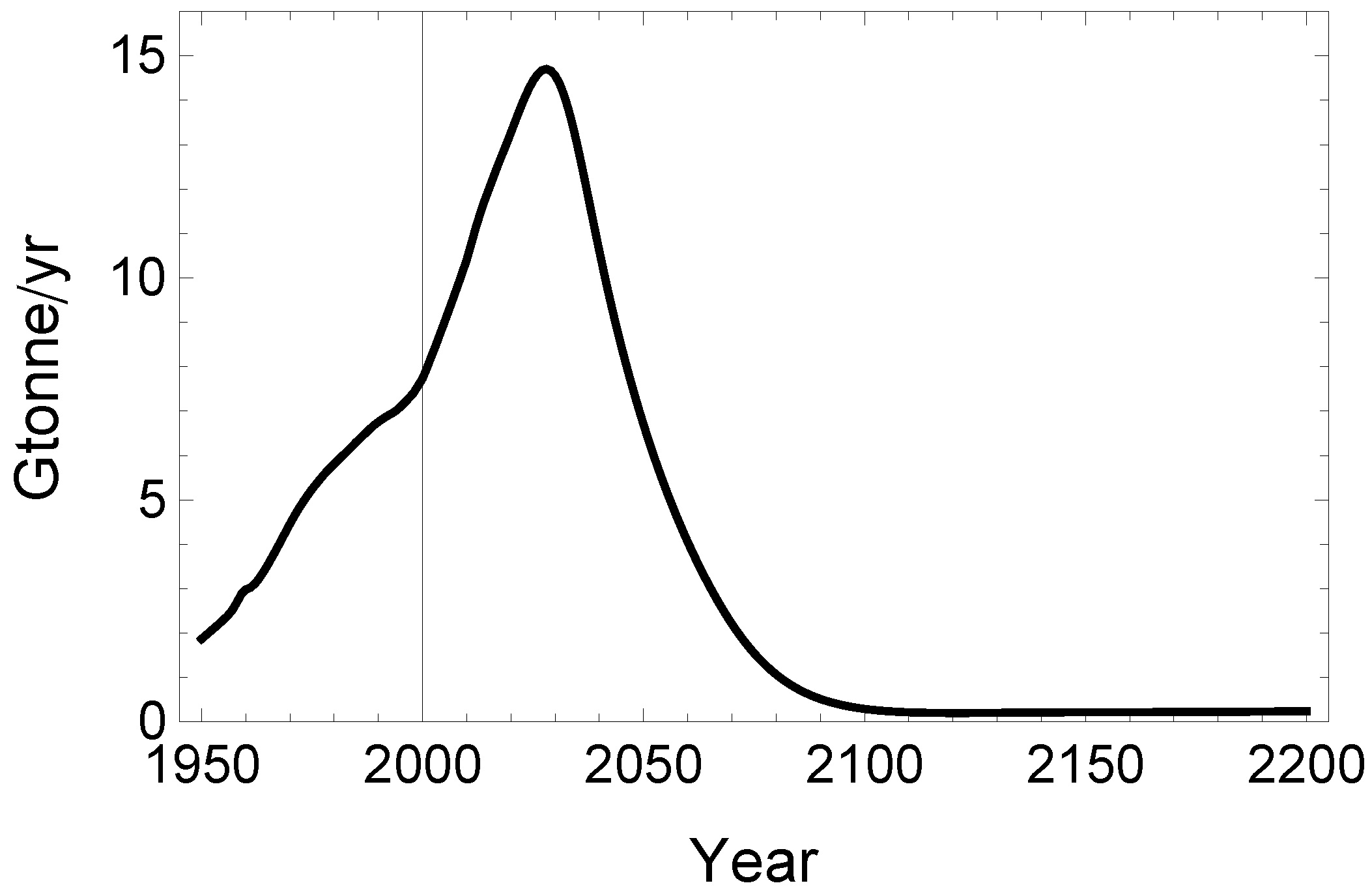
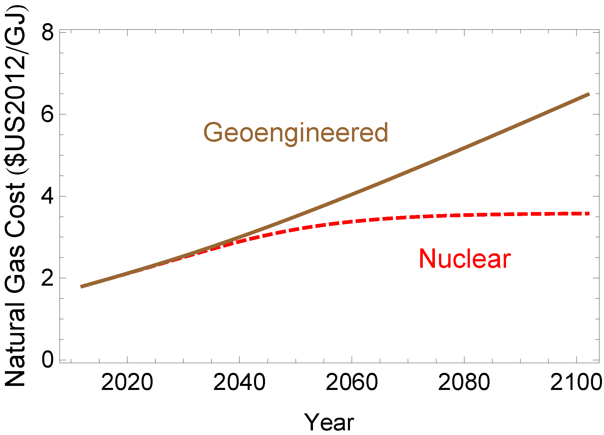
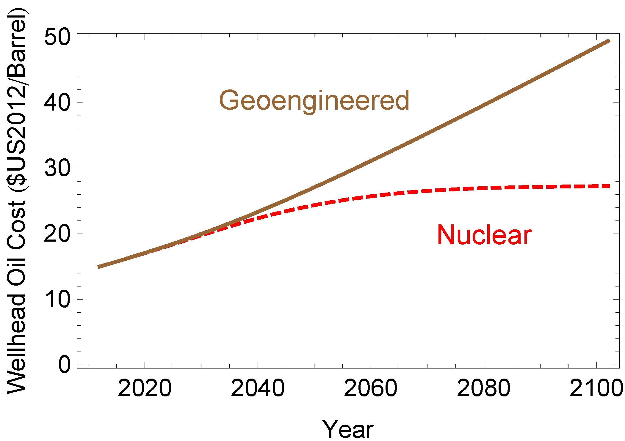
k. The shadow effect is a measure of how expectation of future difficulties with using fossil carbon affect current prices. The results shown in
Figure 4 and
Figure 5 suggest that the time scales for depletion of fossil fuels to escalate prices is long compared to the capitalization time
≈ 7.8 years. It would be interesting to compare the results shown in this paper to data-calibrated integrations from terminal sustainable boundary conditions of the fourth order set of equations obtained without expansion in either
δ or
ϵ, but this demanding exercise is beyond the scope of the present paper. With the approximation used here, the ratio of annual energy use rate to GDP is simply proportional to 1 +
hp.
The solution to the above welfare maximization problem depends on how carbon intensity
p evolves with time. As a first approximation, we use historical time-series data to extrapolate
p as starting at 1 and declining exponentially towards a lower limiting value. That is, the starting points for the iteration are of the form
. Once the resulting total energy use rates are broken down into a different set of constituent sources for each country group, as described below, a new estimate for
p is obtained. The evolution of energy use rates is then re-computed. For the results shown here, a single iteration of this type is used. Normalized to that for coal, the carbon intensity of oil taken to be 0.75 and that for natural gas is taken to be 0.54. Non-fossil electrical energy sources are approximated as having zero carbon intensity. (This approximation is initially sufficient for our purposes, and becomes more accurate as non-fossil energy sources are increasingly used for the industrial inputs to construction of non-fossil electrical energy facilities.) For biofuels we count as energy sources only the net solar energy content of the fuels. This is taken to be 0.6 times the biodiesel combustion energy. For fuel ethanol the net solar energy content is taken to be 0.23 times the combustion energy in temperate regions and 0.875 times the combustion energy in other regions. This is based on an observation that trade between regions producing fuel ethanol primarily from edible food products and from sugar cane tends to be a small fraction of total fuel ethanol use in each country group, and the production of ethanol from sugar cane requires a lower non-solar energy input. Based on historical trends only, each country group has been headed towards a limit carbon/energy ratio, normalized to that for coal, of the values for
D3 listed in
Table 3.
Table 4 and
Table 5 list starting years
Y1 and timescales
Y2 for functions of the form
, including the values of
D1 and
D2.
Table 4.
Starting dates for exponential functions.
Table 4.
Starting dates for exponential functions.
| China | India | Nigeria | Brazil | Ethiopia-Egypt | Indonesia | EU | USA | Japan |
|---|
| D1 | 1935.4 | 1935.9 | 1937.8 | 1912.3 | 1927.6 | 1923.4 | 1945.4 | 1929.6 | 1919.9 |
| E1 | 2002.3 | 2009.5 | 2005.7 | 2003.7 | 2007.0 | 2006.6 | 2003.6 | 2003.7 | 2008 |
| F1 | 2014.8 | 2049.8 | 2067.9 | 1996.3 | 2018.0 | 2009.5 | 1967.8 | 1967.3 | 1952.8 |
Table 5.
Timescales (in Years) for exponential functions.
Table 5.
Timescales (in Years) for exponential functions.
| China | India | Nigeria | Brazil | Ethiopia-Egypt | Indonesia | EU | USA | Japan |
|---|
| D2 | 117.15 | 24.35 | 31.17 | 44.27 | 24.37 | 52.52 | 53.96 | 22.96 | 40.01 |
| E2 | 6.37 | 1.47 | 6.05 | 4.23 | 0.02 | 1.91 | 8.97 | 6.27 | 4 |
| F2 | 5.51 | 21.43 | 21.64 | 11.86 | 17.08 | 17.50 | 11.34 | 13.08 | 10.82 |
Once an iterated estimate for the evolution of carbon intensity
p of energy production is obtained, first approximations to the increases in energy use rates over 1820 levels are
. Here
RE is a different constant for each country group as listed in
Table 6,
are the population increments over 1820 levels, and
B denotes the per capita GDP functions described above. The smooth evolution of energy use rates that these functions describe has been interupted by various events such as China’s “Great Leap," major economic reform, the partition of the Soviet Union, major recessions in the United States, and the 2011 tsunami in Japan. To account for such events, the formula
is multiplied by a different function
ffix for each country group to account for some anomalies that interrupt the overall evolutionary trends. For the China group, the fit to the ratio of annual energy use (in EJ) to GDP (in T$US1990PPP) is multiplied by
where
,
, and
. The factor
f11 accounts changes after the launch of economic reform. The other two factors account for the “Great Leap" period’s energy use inefficiency.
For the India group, . For the Nigeria, Brazil and Indonesia groups, ffix = 1. For the EU group, the presumably unique events associated with the partition of the Soviet Union give for ffix. For the USA group, accounts for the impact of two major recessions. For Japan there is a transient energy use rate above the background trend preceding the 1973 oil price increase and a presumably transient decrease associated with recent economic upsets including the 2011 tsunami. To account for this events, the formula for ffix for Japan is set to where , , and . The long-term limits for the functions ffix are equal to 1 except for 0.743 for the China group, 0.837 for the EU group, and 0.630 for the USA group. These numbers give some idea of the minimum uncertainty in the long-term extrapolations, since different results differing by the magnitudes for which some of the long-term ffix differ from 1 would be expect to result from using different functional forms ffix (e.g., allowing for the possibility of future major recessions in the USA group).
D. Energy Sources
The division of total energy use rates into different energy sources starts with conventional biofuels. The sum of annual conventional (biodiesel and non-cellulosic ethanol) biofuels consumption in each region is approximated as nil until a time
E1 and of the form
thereafter. The same type of formula,
, is used for water-driven electrical energy, with the long-term limit from estimates of hydropower potential capacity [
18] times the ratio of U.S. actual hydropower to potential capacity. (Tidal and geothermal electric energy capacities are assumed to be so small in comparison to uncertainties in hydroelectric capacity that they do not need to be accounted for separately when prescribing the long-term limit rates of consumption of water-driven electricity.) These contributions to energy use are assumed to be limited by suitable cropland and watershed availability and thus are not proportional to total energy use.
The fraction of total thermal equivalent energy from nuclear reactors in each region is approximated as evolving as . Except for India and Japan, fon = 1. For India, , and for Japan . Except for Japan, foff = 1. For Japan, . For the India group, including the factor fon helps fit the nearly linear build up of nuclear energy use from 1990 to 2010. For Japan, the parameters in fon and foff are chosen to model the expected effects of the year 2011 tsunami.
The fraction of total thermal equivalent energy consumption rate from new renewables (wind- and solar-electric energy) is approximated for each region as nil for
ty <
I1, and as
for
ty >
I1. Here
Etotal is cumulative energy use in EJ each region after year
I1. The values of the constants in this formula are given in
Table 6, with the units of the value for
I5 being EJ. This formula results from assuming that the fraction of the total energy market in each region that is acquired by new renewables is proportional to an exponentially saturating function
of cumulative production
W from new renewables (which are so far mostly wind energy). Due to the limited experience of the Nigeria group with new renewable electrical energy sources, the fraction of total energy from those sources is set to its year 2012 value of 0.000137 instead of using the formula corresponding to the parameters in
Table 6. This limitation for the Nigeria group is a reflection of limited infrastructure for managing grid-connected wind and solar electric energy production. This is in a context where the substitution of wind and solar energy sources for wood and other energy sources not included in our database is assumed to be part of the “preindustrial” part of the economy that is not analyzed here because such substitutions are approximated as not materially affecting global fossil carbon burning.
The total cumulative fossil energy use
Efossil is calculated for each region as total thermal equivalent energy use less the thermal equivalent of the non-fossil energy sources estimated as described in the preceeding three paragraphs. The cumulative use
Eff of fluid fossil fuels solves the equation
, subject to the boundary condition that
Eff is equal to the cumulative use
J3 of fluid fossil fuels through 2012 as estimated from the database. The values of
J1,
J2 and
J3 are listed in listed in
Table 6, with
J2 and
J3 in EJ. It is convenient to integrate this equation numerically. The same applies to the natural gas fraction of fluid fossil fuels, discussed in the next paragraph.
As a first approximation, the cumulative consumption
Egas of natural gas solves the equation
, subject to the boundary condition that
Egas is equal to the cumulative use
K3 of fluid fossil fuels through 2012 as estimated from the database. The results of this calculation for
Egas/
dt are multiplied for each region by an empirical correction factor of the form
. The values of the constants in these formulas are listed in
Table 6. To account for the presumably partly temporary shut down of Japanese nuclear reactors following the 2011 tsunami, for Japan an additional multiplicative factor of
was included. Here 0.487 is an estimate of the fraction of Japan’s nuclear capacity that will come back on line if all of its pressurized water reactors and advanced boiling water reactors restart, but the remaining reactors do not (based on reported reactor capacities [
19]). For 2010 through 2012, the Nigeria group’s natural gas consumption was much lower than in the eleven preceding years. This was because exports of liquefied natural gas continued despite the shut down of a large Nigerian natural gas production facility [
20]. Unlike the expected extensive shutdown of about half of Japan’s nuclear reactor fleet, the disruption of natural gas consumption in Nigeria is assumed here to be temporary and thus not accounted for with another special multiplicative factor. Disruption of Libyan natural gas consumption in 2011 and 2012 and reductions in Iranian natural gas consumption from 2010–2012 were also assumed to be temporary and thus not accounted for with a special multiplicative factor.
Table 6.
Region-dependent constants for experiential learning.
Table 6.
Region-dependent constants for experiential learning.
| China | India | Nigeria | Brazil | Ethiopia-Egypt | Indonesia | EU | USA | Japan |
|---|
| I1 | 1990 | 1986 | 2002 | 1990 | 1986 | 1990 | 1978 | 1999 | 1995 |
| I2 | 0.064 | 0.070 | 0.030 | 0.067 | 0.057 | 0.056 | 0.061 | 0.068 | 0.055 |
| I3 | 2.651 | 1.498 | 0.026 | 0.234 | 0.231 | 0.517 | 11.793 | 5.947 | 0.518 |
| I4 | 26.73 | 8.18 | 3.90 | 7.53 | 8.32 | 9.94 | 37.27 | 26.18 | 6.63 |
| I5 | 10.59 | 5.98 | 149.08 | 32.64 | 36.54 | 19.72 | 3.68 | 4.92 | 13.31 |
| J1 | 0.211 | 0.582 | 0.504 | 0.939 | 0.936 | 0.736 | 0.706 | 0.782 | 0.785 |
| J2 | 5.90 | 9.53 | 4.62 | 5.71 | 1.90 | 10.29 | 312.90 | 200.83 | 13.26 |
| J3 | 503.7 | 517.5 | 190.9 | 930.8 | 936.8 | 689.8 | 3944.0 | 4185.6 | 559.6 |
| K1 | 0.201 | 0.464 | 0.331 | 0.338 | 0.504 | 0.329 | 0.531 | 0.428 | 0.362 |
| K2 | 28.1 | 33.3 | 17.0 | 35.6 | 8.8 | 31.3 | 330.6 | 0.3 | 49.7 |
| K3 | 62.1 | 214.7 | 45.8 | 306.5 | 444.9 | 185.5 | 1552.8 | 1734.5 | 91.7 |
| L3 | 0.55 | 0.35 | 1.2 | 0 | 0.15 | 0.66 | 0.42 | 0.11 | 0.6 |
| L4 | 0.43 | 0.60 | 0.2 | 1.03 | 0.98 | 0.38 | 0.60 | 0.89 | 0.01 |
| RE | 6.64 | 4.51 | 6.85 | 5.18 | 8.66 | 4.62 | 7.48 | 7.16 | 4.18 |
For the case where future nuclear energy use is dramatically increased rather than relying on stratospheric sulfur injection later supplemented with extensive carbon sequestration, the nuclear energy use fraction described above is multiplied by a factor
. Here
flate = 1, except that
flate is set equal to
and
respectively for the slowly developing Nigeria and Brazil groups. The other constants used in this formula are given in
Table 7.
Table 7.
High nuclear case multiplier constants.
Table 7.
High nuclear case multiplier constants.
| China | India | Nigeria | Brazil | Ethiopia-Egypt | Indonesia | EU | USA | Japan |
|---|
| M1 | 2035.5 | 2052 | 2067 | 2067 | 2052 | 2062 | 2050 | 2042 | 2052 |
| M2 | 5 | 10 | 10 | 10 | 10 | 10 | 6 | 6 | 10 |
| M3 | 57.5 | 58.7 | 99.0 | 77.0 | 165.0 | 27.1 | 10.75 | 11.7 | 12.7 |
E. Global Heat and Carbon Balances
Milligan [
21] describes an adaptation of a global heat balance model due to Fraedrich [
22] to solve for a temperature anomaly
τ =
T −
T0, where
T0 = 286.48°K and
T is global average temperature in °K:
Here
ts is time in seconds from the beginning of Julian year 1000,
I0 = 1, 366 W/m
2 is the time-averaged solar irradiance, and
σ = 5.6704 × 10
−8 W/(m
2 °K
4) is the Stefan-Boltzman constant. The temperature dependence of the albedo is determined by
a2 = 1.160 and
b2 = 1.045 × 10
−5/(°K)
2, which give an albedo of 0.30 when
T =
T0. The temperature-dependent part of the effective emissivity,
, is determined by the value of
κ = 3 × 10
−6/(°K)
2. The effective emissivity is also influenced by the atmospheric CO
2 concentration through the relationship
. Here [CO
2]
0 = 280 ppmv and [CO
2] is the atmospheric CO
2 concentration in ppmv. The constant
e1 = 0.00688 determines CO
2 forcing of global average temperature in the context of this model and was adjusted to give a equilibrium carbon forcing increment in
τ of 3.0°K for a doubling of atmospheric CO
2 concentration from 280 ppmv to 560 ppmv [
23]. The ocean mixed layer thermal inertia constant is
cheat =
foceanρseaCpdmixed, where
focean = 3.6/5.1 is the fraction of the earth’s surface area covered by ocean, the seawater density is
ρsea = 1, 027 kg/m
3, and
Cp = 3. 985 J/(kg °K) is the heat capacity of sea water. An ocean mixed layer depth of 335 m was chosen to fit global average temperature data from 1850–2013. This was done by choosing the integer value in meters for
dmixed that minimized variance between the computed and observed results, while also adjusting a constant offset between data and computation to minimize variance.
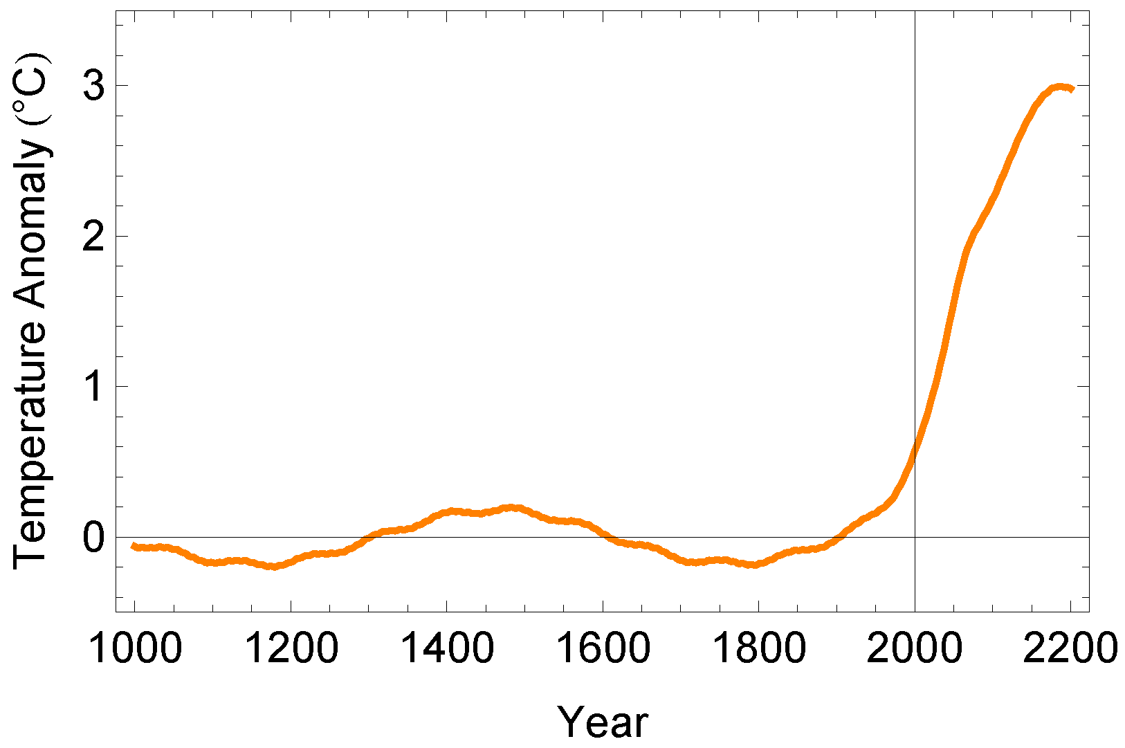
Oscillations in solar irradiance are given by
, where
ty is time in Julian years. These oscillations are all in phase at maximum when
uy = 1, 994.3 Julian years. The four periods are 2
π/
ωj = {11, 22, 88, 600} years, and the respective amplitudes
ρj are {0.25, 0.05, 0.2, 0.4}/1, 000. These amplitudes determine the size of the preindustrial variations in
τ shown in
Figure 2. These amplitudes are smaller than early estimates by Lean
et al. [
24] used by Milligan [
21], and more in line with more recent estimates by Steinhilber
et al. [
25].
The annual rate of change of the sum
ca +
cw +
cv +
cs of carbon respectively in the atmosphere, surface ocean water, vegetation, and soil is set equal to the difference
Rf −
Rm between the global fossil carbon emission rate,
Rf, and the rate
Rm of removal of carbon from the surface mixed ocean layer to the deep ocean due to the difference between
cw and its preindustrial average value
cw0. That rate is
Rm = (
cw −
cw0)/
tm with
tm = 173 years [
23]. Equilibration between the atmosphere and surface ocean layer is assumed to occur rapidly enough to be approximated algebraically as in equilibrium [
26]. Two of the remaining three differential equations are
dcs/
dty =
Rℓ −
Rs for soil and
dcv/
dty =
Rp −
Rv −
Rℓ for vegetation. Defined below are the rates
Rℓ,
Rs,
Rp and
Rv of carbon transfer respectively from litter fall, soil respiration, photosynthesis, and respiration by vegetation. (We have not attempted to model the effect of land use changes on carbon in vegetation, as this difficult to extrapolate.) The relationship between the molar concentration
cw/
vm in the surface ocean mixing layer and the volume fraction
ca/
va in the atmosphere depends on the ratio
z1 of the bicarbonate dissociation constant
k1 to the hydrogen ion activity
aH as
Here vm is 4.348 times the surface ocean mixing layer depth in meters, and va = 2, 130 ppmv per Ttonne of elemental carbon.
The temperature dependence of the solubility constant, bicarbonate dissociation constant, and carbonate dissociation constant,
, are respectively
where
Tc is the temperature on the Celsius scale. The salinity is approximated as
Sppt = 35. Accounting for borate buffering from a total molar boron concentration of
Bm = 0.004106 and dissociation constant
with
, the ratio
z1 satisfies the cubic equation
.
Since derivatives of
z1 with respect to
Tc need to be chain-rule coupled to time derivatives of
Tc, it is convenient to pick out the physically appropriate root of the cubic equation for
z1. This root is given by
z1 =
sz +
tz −
a2/3 where
and
with
,
, and
. The expressions for the coefficients in the cubic equation are
where
Acb = 0.00223.
With the above algebraic relations in hand for the dependence
of the ocean mixed layer carbon content on atmospheric carbon content and temperature, one can write the rate of change of the sum of atmospheric and mixed ocean layer content as
plus
where
. With the above equations
for soil and
for vegetation, we can then include
The fractional carbon respiration rate
, and fractional vegetation carbon respiration rate
increase respective by factors of
and
for a 5 °C of temperature increase photosynthesis are respectively, and they have carbon turnover timescales respectively of 30 and 11 years. The litter fall carbon rate is simply
. The rate of carbon uptake into vegetation depends both on temperature and atmospheric carbon content. Inclusion of the constant
in the following expression for
Rp is a consequence of not accounting for any change in the areal extent of vegetation cover.
The coupled global carbon and heat balance equations are integrated forward from Julian year 1000, with starting conditions −0.062429 °C for τ, for 1.5 Ttonne for ca, 0.55 Ttonne for cv, and 0.55 Ttonne for cs.
G. Databases
The data for GDP for the years 1820–2008 are from Maddison [
16]. GDP estimates are in purchasing power parity in year 1990 U.S. dollars. For later years, International Monetary Fund [
27] estimates and projections through 2018 were multiplied by a constant for each country to make those estimates consistent with the last year available in Maddison’s database. For groups of countries where Maddison gave only aggregate estimates of population and GDP, these were disaggregated in proportion to UN estimates for each country. Since the present paper re-aggregates countries into larger groups, the method of disaggregation of Maddison’s estimates has negligible effect on the results presented here. Allowing for a period of relaxation for areas involved in World War II, GDP data used started in 1961. Exceptions to the 1961 date are 2001 for the China group and 2003 for the India group, since the effects of earlier economic reforms showed up as a pronounced change in the rate of growth of per capita GDP in those years. For the Indonesia group the start year for GDP data use was 1967, before which per capita GDP growth rates were anomalously low.
The year 1820 value for population and GDP for each country group is subtracted from the data. The result for population is used to calibrate three parameters in a logistic fit. These are the initial exponentiation growth time, the time to half maximum, and the long-term limit value. The fit is accomplished by minimizing the variance of the difference between the logarithm of the data and the logarithm of the fitting function. The same procedure was used to fit data on the ratio of the GDP increment over 1820 values to the population increment over 1820 values.
The database for energy use rates has annual estimates from 1820–2012 for eleven parameters for each UN reporting unit (mostly but not all sovereign countries), except that Sudan and South Sudan are included together. These data are combined into the seven different energy types as described above. (For current countries previously part of larger reporting units, the earlier data is divided in proportion to split at the time of division, but for the results in the present paper all of these cases are re-aggregated into larger country groups.) Country-specific data from 1950–2010 are from the United Nations Energy Database [
28]. For years after 2010, U.S. Energy Information Agency estimates [
29] were used where they were available and British Petroleum estimates [
30] where used where not, both scaled with a multiplicative factor to match the year 2010 UN estimates. For countries missing from the British Petroleum database, their portions of the BP regional sums not accounted for by individual countries in those sums were allocated in proportion to the most recent data available from other sources. Cumulative energy consumption rates from before 1950 were summed annual estimates based on Mitchell’s
Historical Energy Statistics [
31], the UK statistical summaries of the mineral industry [
32] and British [
33] and U.S. [
34] trade tables for exports of coal and oil by destination. The cumulative energy consumption rates before 1950 and the annual energy use rates from 1950–2012 for the above-mentioned seven energy types and the nine country groups are included in a table of supplementary material accompanying this paper.


