Article

Low-Cost Non-Contact Forest Inventory: A Case Study of Kieni Forest in Kenya

1
Department of Electrical and Electronic Engineering, Dedan Kimathi University of Technology, Dedan Kimathi, Nyeri P.O. Box 10143, Kenya
2
Centre for Data Science and Artificial Intelligence (DSAIL), Dedan Kimathi University of Technology, Dedan Kimathi, Nyeri P.O. Box 10143, Kenya
3
NVIDIA Corporation, 2701 San Tomas Expressway, Santa Clara, CA 95050, USA
*
Author to whom correspondence should be addressed.
Challenges 2024, 15(1), 16; https://doi.org/10.3390/challe15010016
Submission received: 11 August 2023 / Revised: 5 March 2024 / Accepted: 6 March 2024 / Published: 18 March 2024

Abstract

:
Forests are a vital source of food, fuel, and medicine and play a crucial role in climate change mitigation. Strategic and policy decisions on forest management and conservation require accurate and up-to-date information on available forest resources. Forest inventory data such as tree parameters, heights, and crown diameters must be collected and analysed to monitor forests effectively. Traditional manual techniques are slow and labour-intensive, requiring additional personnel, while existing non-contact methods are costly, computationally intensive, or less accurate. Kenya plans to increase its forest cover to 30% by 2032 and establish a national forest monitoring system. Building capacity in forest monitoring through innovative field data collection technologies is encouraged to match the pace of increase in forest cover. This study explored the applicability of low-cost, non-contact tree inventory based on stereoscopic photogrammetry in a recently reforested stand in Kieni Forest, Kenya. A custom-built stereo camera was used to capture images of 251 trees in the study area from which the tree heights and crown diameters were successfully extracted quickly and with high accuracy. The results imply that stereoscopic photogrammetry is an accurate and reliable method that can support the national forest monitoring system and REDD+ implementation.

1. Introduction

Forests contribute positively to people’s daily lives worldwide by being a source of food, medicines, and fuel. They also protect the world’s watersheds, maintain soil structure, and function as carbon stores [1]. Since forests are the dominant plant biomass source, 50% of which comprises carbon, they play a critical role in the carbon cycle [2]. Forests are also important for aesthetic, educational, spiritual, and recreational reasons [3]. Establishing and monitoring forests also significantly contributes to the United Nations (UN) Sustainable Development Goal (SDG) 13 on climate action.
Forest monitoring and conservation are needed to help sustain these benefits [3]. Forest monitoring involves measuring and recording tree-level biophysical parameters and stand-level attributes in a forest inventory. Forest inventories are the primary information sources used in forest management and for forestry policy formulation [4,5,6,7,8]. Total tree height (TH) and diameter at breast height (DBH) are the two most common tree attributes in forest inventories [9]. From these two, other attributes such as above-ground biomass (AGB), timber volume, and basal area can be derived [6,9,10,11]. Crown diameter (CD) and crop height are usually of interest in precision agriculture [12]. Comprehensive forest monitoring requires a combination of remote sensing techniques, such as the use of satellite imagery as well as field data collection at the plot level. Remote sensing is useful for forest monitoring at scale, e.g., forest cover estimation. At the same time, field data collection gives more granular data, such as trunk diameters, tree heights, and basal area, from which biomass and carbon stocks are calculated. Satellite imagery has been used to estimate forest biomass as forests are critical to efforts to reduce carbon emissions [13,14]. Unfortunately, satellite data often result in unreliable forest biomass estimates and can overestimate above-ground biomass by up to an order of magnitude [15].
Remote sensing is widely applied in forest monitoring in many countries globally [16,17]. For example, the Global Forest Watch maintains a near-real-time online system on global forest cover, with its data sourced mainly through remote sensing approaches [18]. Despite the widespread adoption of remote sensing in forest monitoring, certain geographical regions are lagging in its uptake, particularly developing nations [1,3,6,7,17]. To address this, experts suggest leveraging emerging technologies, noting that countries with robust monitoring systems, such as Norway, Finland, and Sweden, have usually been early adopters of new forest inventory technology [17,19]. The calibration of empirical remote sensing models with plot-level ground truth measurements is essential, further underscoring the need for improved speed and efficiency in these measurements [17,20]. Since the remote sensing approach lacks the granularity found in national forest inventory data, efforts to bridge this gap are crucial for comprehensive and accurate forest monitoring.
National forest inventories (NFIs) provide high-quality data on national forest resources with a high degree of accuracy and detail. Therefore, many countries regard them as the best sources of information about their forest sectors [5]. Norway, Sweden, and Finland lead the way with the oldest and most robust NFIs, and they have maintained robust forest monitoring systems [5,7,17]. One widely adopted practice in forest inventory is the use of sample plots for collecting plot-level attributes [11,17,21,22]. Plot-level measurements collected from sample plots lend themselves to application in statistical estimators used in NFIs and in calibrating empirical and machine learning prediction models used in remote sensing tools [17]. This helps improve the accuracy of remote sensing approaches, which, although very suitable in situations where scale is a primary consideration [3,17,20], are known to fall short in measuring under-canopy attributes [16,17,20]. As such, field surveys will continue to be a necessary component of forest inventory surveys for the foreseeable future [20]. Accurate forest inventory data are required to compute accurate biomass and carbon stock data.
A thorough knowledge of carbon stock information is critical in initiating and sustaining plans for climate change mitigation, such as under the REDD+ framework and in laying strategies for bioenergy production [23,24,25]. This information is usually missing or grossly inaccurate in many developing countries owing to the unavailability of reliable forest inventory data [3,7]. Some studies that have been conducted in Kenya to estimate the above-ground biomass (AGB) stocks are not up to date, and the result is that detailed, complete, and rigorous assessments of AGB stocks are not easy to find [25,26]. These studies also show disconcerting planetary health challenges, such as a decline in forest cover and biodiversity loss across various regions [27,28,29,30,31,32], mainly due to increasing population pressure and demand for agricultural land that has led to deforestation [29,30,33,34]. The decreasing forest cover has decimated the amount of AGB and carbon stocks in the country [25,26,35]. Therefore, finding the best strategies for enhancing forest conservation and monitoring is imperative.
One of the strategies for enhancing conservation is the involvement of forest-adjacent communities in decision making and planning. This has been shown to increase the sense of ownership over forest resources, thereby fostering a stronger commitment to conservation [36,37,38,39]. The forest management approach significantly shapes the availability, access, and utilisation of forest products and the extent of community engagement in conservation efforts [36]. Notably, the involvement of community forest associations in conservation contributes to a heightened perception of the importance of forest ecosystems [36,39]. Moreover, communities allowed to access and utilise forest products demonstrate increased participation in conservation initiatives [36,37]. The continued co-management of forest resources shared between the government and community organisations is a highly recommended sustainable management strategy [36,40,41]. Another sustainable practice is revegetation using native species instead of exotic ones due to its effectiveness in preventing soil degradation and hydrological changes, thus presenting a synergistic approach to forest technology [42].
Several studies on land cover changes in various parts of Kenya have observed an initial increase in forest cover from 1995 to 2001 due to government policy. However, after 2001, there was a steady decline in forest cover. To achieve and maintain the required 10% forest cover as per constitutional and UN requirements, researchers recommend adequate and consistent afforestation and reforestation efforts [30,31,32,33,34,37,39]. Acting upon these recommendations, Kenya’s parliament passed the Forest Conservation and Management Act in 2016, and the result has been an increase in forest cover [25,30,31,37,43]. The country’s national strategy includes enhancing forest resource assessment through a comprehensive national forest inventory, an endeavour which requires capacity building for remote sensing surveys and field data collection [21,30,31,39,40,43,44]. The responsibility for realising this lies with the Kenya Forest Service, Kenya Forestry Research Institute, and universities [43]. Given Kenya’s ambitious objective of increasing its forest cover to 30% by 2032, the need to closely monitor and assess the growth of these young stands has never been more apparent. This study describes a forest inventory exercise carried out in Kenya using a low-cost, non-contact approach.
Forest inventories often involve complex variables that require significant effort, expertise, and subjective estimates from field staff [10]. Researchers have explored non-contact methods that utilise digital image and point cloud processing to overcome these challenges. Prominent techniques include structure from motion (SfM), laser scanning, and simultaneous localisation and mapping (SLAM). However, these methods are typically slow, expensive, and computationally intensive [45]. Ideal measurement techniques should be fast, accurate, practical, and cost-effective. SfM reconstructs 3D scenes from a series of images using multiple-view geometry principles [9,46,47,48,49,50]. Nevertheless, its measurement accuracy decreases with distance [12,46,47,48,51]. Laser scanning with LIDAR cameras is a popular remote sensing tool in forestry due to its high precision [52] and has been applied in some forest inventory studies [52,53,54,55,56,57,58,59,60]. Although laser scanning is widely used in forest inventory studies, the expensive cost of LiDAR cameras hinders broader adoption [50,57,58,59,60,61]. Although less commonly applied in tree inventory, SLAM has been used in some studies [62,63].
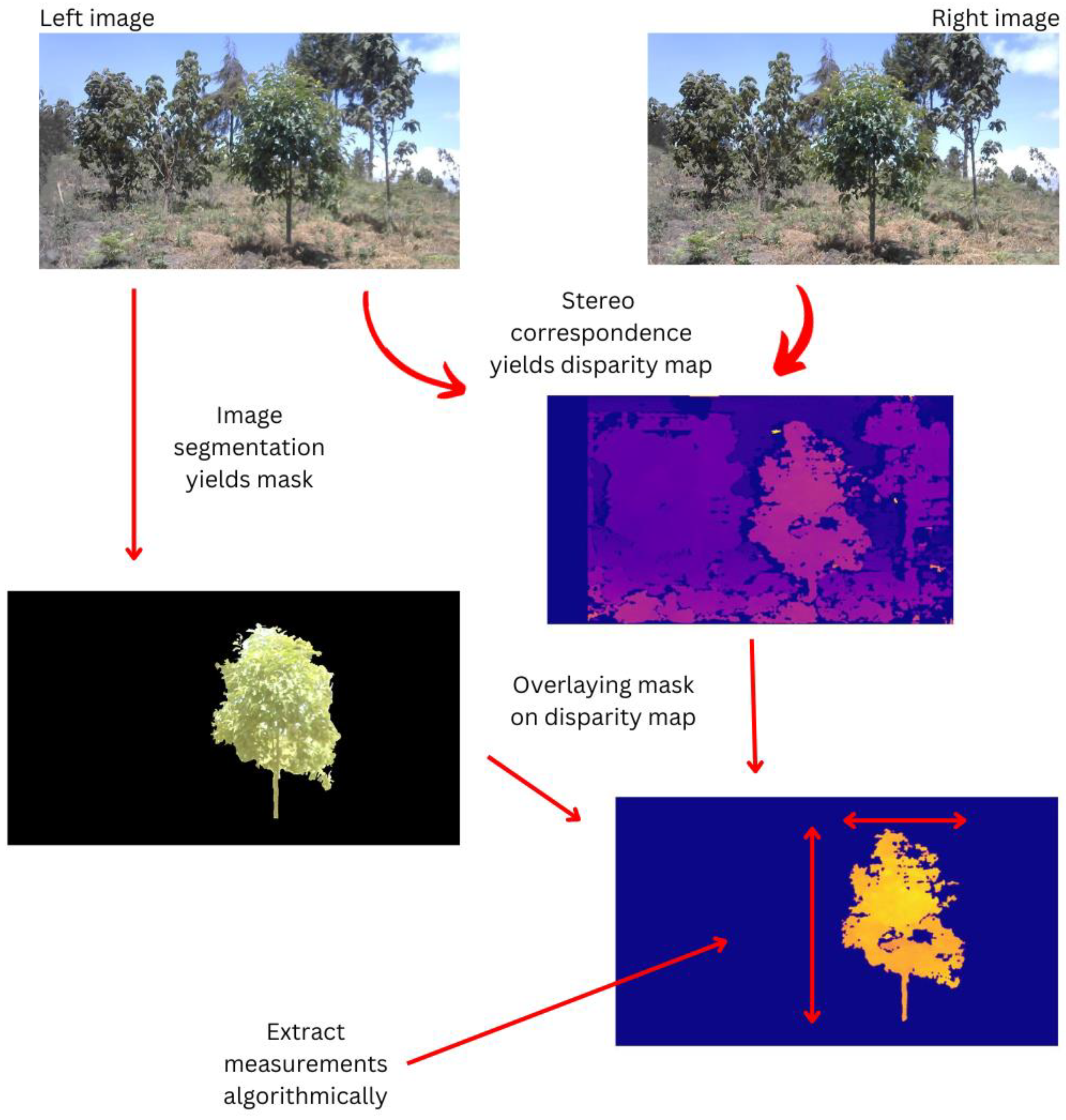
One attractive method of non-contact tree inventory that provides an alternative to the aforementioned techniques is stereoscopic photogrammetry. This involves obtaining the geometric information of a scene from a pair of overlapping images [64,65,66]. It offers the advantages of low cost, good accuracy, and low computational cost [64,67]. Although its application in inventory is still a growing area of research, it has been applied in several studies to estimate the biophysical parameters of trees [45,57,59,64,68,69,70,71,72,73,74,75]. This approach was used to conduct non-contact tree inventory in this study.
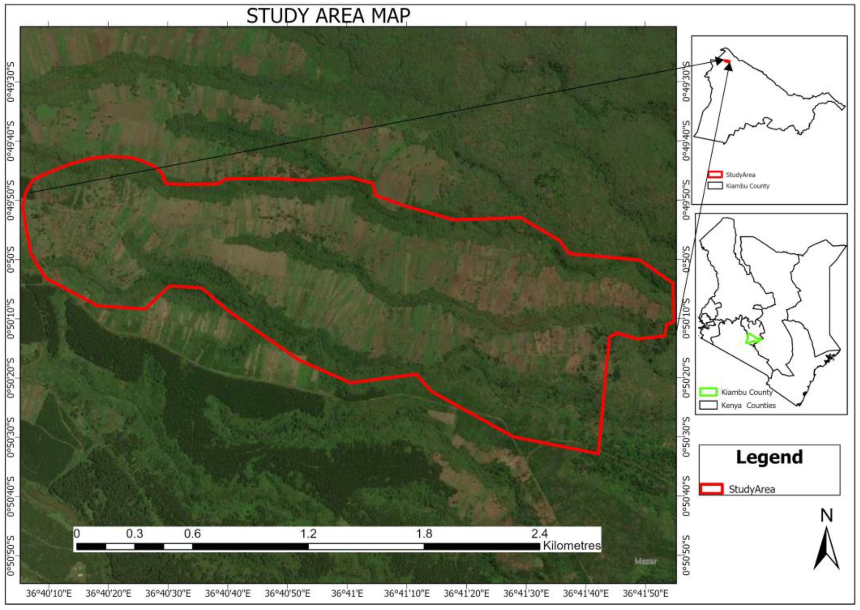
This study was conducted in a reforested stand within the Kieni Forest in Kenya to assess the applicability of stereoscopic photogrammetry in collecting forest inventory data for Kenya to automate, expedite, and ease the process of performing field data collection in forest inventory exercises. The rest of this paper is organised as follows: Section 2 presents the methodology used in this study; Section 3 contains the results; Section 4 discusses the results and the limitations of our research; and Section 5 presents the conclusions arrived at and points out directions for future work.

2. Materials and Methods

2.1. Study Area

Kieni Forest is one of the forest zones that comprise the Aberdare Forest Ecosystem, located on the Aberdare Ranges (see Figure 1). It is managed by the Kenya Forestry Service (KFS). The Aberdare Ranges is one of Kenya’s five main water towers and supplies approximately 80% of the water used in Nairobi through the Ndakaini and Sasumua dams. The entire ecosystem spreads across four counties—Kiambu, Murang’a, Nyeri, and Nyandarua—with Kieni Forest located within Kiambu. Kieni Forest lies between 2200 m and 2684 m above sea level and receives rainfall of 1150 mm to 2560 mm annually [76]. The long rain season stretches from March to June, while short rains are received from October and December. Its soils are rich in organic matter, making them fertile and favourable to developing thick undergrowth. Its vegetation comprises natural forests, plantations, bamboo, meadows, and tea zones [77]. The replanted section covers an area of 269 ha and contains more than ten indigenous species, mainly Dombeya torrida, Juniperus processera, Olea africana, and Prunus africana. The crown diameters range from 0.4 m to 4.7 m, while the heights range from 0.75 m to 5.0 m. Being a reservoir of biodiversity, Kieni Forest also has a wide range of fauna, such as the African elephant (Lexodonta africana), duiker (Neottragus moschatus), Bush pig (Patomochoerus porcuso), and mongoose (Helogale parvula), among others [76,77].

2.2. Materials

The stereo images were captured using a stereo camera comprising two Logitech C270 USB web cameras, which have a resolution of 720 × 1280 pixels, in an assembly. A custom-designed and 3D-printed rig was used to hold the two web cameras together with a baseline of 12.9 cm. To capture the images, the stereo camera was accessed using a custom-built software tool featuring an easy-to-use graphical user interface (GUI). The images were also processed using the same tool. This application is available as an open-source tool [78] that is useful for extracting tree biophysical parameters. This application was run on an NVIDIA Jetson Nano 2 GB Developer Kit with an HDMI mini screen. The features of this kit include a quad-core ARM A57 @ 1.43 GHz processor, 4 GB 64-bit LPDDR4 RAM, and a 128-core Maxwell GPU (NVIDIA Developer, Santa Clara, CA, USA). The application was built using the Python programming language [79], with the OpenCV [80] library used for image processing and computer vision tasks and the Kivy library [81] used for building the user interface.

2.3. Terrestrial Stereo Photogrammetric Survey

The CD and TH estimation images were captured at the designated study area during the field data collection exercise in March 2023. The weather conditions on those days were mostly calm, cloudy, and sunny on a few occasions. The study area was a recently replanted section of a forest comprising sapling trees with trunks mostly covered by twigs or too slender to be measured. Therefore, the technique’s performance at DBH estimation was evaluated using images of tree trunks surveyed during a test run conducted at the Dedan Kimathi University of Technology. The acquisition setup used is described in Section 2.2. In total, 251 stereoscopic image pairs of full trees for CD and TH estimation and 90 stereoscopic image pairs of tree trunks were captured. The images were taken with the camera positioned at arbitrary distances from the tree in all cases.

2.4. Data Processing Pipeline

The process of extracting the tree attributes from the images happened in a series of steps captured in the workflow diagram shown in Figure 2. The images were first captured using a stereo camera and stored in the Jetson Nano kit. These images were then filtered to remove digital noise and then rectified. Rectification is a process performed to ensure the pair of images is correctly aligned. A new image known as a depth map is computed from the rectified images. Each pixel’s intensity in the depth map encodes the depth of that pixel relative to the stereo camera, making it possible to estimate the coordinates of all points in the depth map concerning the stereo camera. The depth is then segmented to retain only the object of interest, in this case a full tree or tree trunk, from which parameters such as diameter at breast height, crown diameter, and tree height are extracted algorithmically. Finer details about the algorithms used for computing the depth map and extracting the tree biophysical parameters are provided in Appendix A.
Figure 3 shows an example of one tree captured at the study area as it goes through the processing pipeline. A binary segmentation mask is obtained by segmenting the left image of the stereo pair. Afterwards, stereo correspondence is performed to yield a disparity map, an image whose pixel intensities represent the depths of those points in the scene (relative to the camera). We obtain a segmented disparity map containing only the three pixels by overlaying the mask on the disparity map. It is from this image that the tree’s biophysical parameters are extracted. A similar process is followed in the case of a tree trunk.

2.5. Performance Evaluation

The performance parameters used to evaluate the performance of our technique include the mean absolute error (MAE), mean absolute percentage error (MAPE), bias, root mean square error (RMSE), coefficient of determination ( R 2 ), and regression line slope. These performance metrics are highly recommended for evaluating the performance of non-contact techniques at biophysical parameter estimation [82].

2.6. Reference Data Collection

Ground truth values of the three tree measurements were recorded during the field data collection exercises and later used as the benchmark against which the values predicted by our method were compared. The exercise was conducted over three days.

2.6.1. Crown Diameter (CD)

The CD was measured by projecting the crown edges to the ground and measuring the length between the edges along the axis of the tree crown to the nearest centimetre using a measuring tape.

2.6.2. Tree Height (TH)

Tree height is the vertical distance between the highest point on the tree and the trunk base, a measurement different from the trunk length, which would be longer for leaning trees. To measure the tree’s height, a graduated pole was placed at the tree base, and the reading at the tip of the tree was recorded.

2.6.3. Diameter at Breast Height (DBH)

The diameter at breast height (DBH) is the tree trunk’s diameter taken at approximately 1.3 m from the trunk base. It is measured by taking the circumference of the trunk at that point using a measuring tape and calculating the diameter or by taking the average of two perpendicular diameters measured using a vernier calliper. In this study, the measuring tape approach was used.

3. Results

3.1. Sample Proportions per Species

After randomly sampling the 251 trees of different species, Juniperus procera, Dombeya torrida, and Olea africana had the highest proportions, at values of 15.1%, 14.3%, and 13.9%, respectively. The fewest trees belonged to the Hagenia abyssinica species.

3.2. Distribution of Measurements across Species

The distribution of the values of crown diameters and tree heights of trees in the study area is captured in the boxplots shown in Figure 4. Most species had their mean crown diameters falling from 100 to 200 cm. The species with the widest trees were Croton macrostychus and Hagenia abyssinica, with mean CD values of 291.25 cm and 270 cm. There were as many species with average heights in the 100 cm to 200 cm range as in the 200 cm to 300 cm range. The tallest trees were Croton macrostychus and Dombeya torrida, with mean TH values of 294.38 cm and 253.06 cm, respectively. The Dombeya torrida species had the largest outliers in tree heights, with trees as tall as 5 m.

3.3. Biophysical Parameter Estimation

The estimated values of the DBH, CD, and TH were evaluated against the ground truth values, and a summary of this evaluation is provided in Table 1. The crown diameter and tree height metrics were calculated using data from the 251 trees surveyed in the study area. In contrast, the DBH metrics are based on the images captured during the test run at the Dedan Kimathi University of Technology. The regression plots for the DBH, CD, and TH are shown in Figure 5. The technique’s performance in TH estimation was comparatively lower than that for CD in most metrics. Overall, a high correlation was observed between extracted and ground truth values of all the parameters, as seen by the R 2 values and the regression plots.

4. Discussion

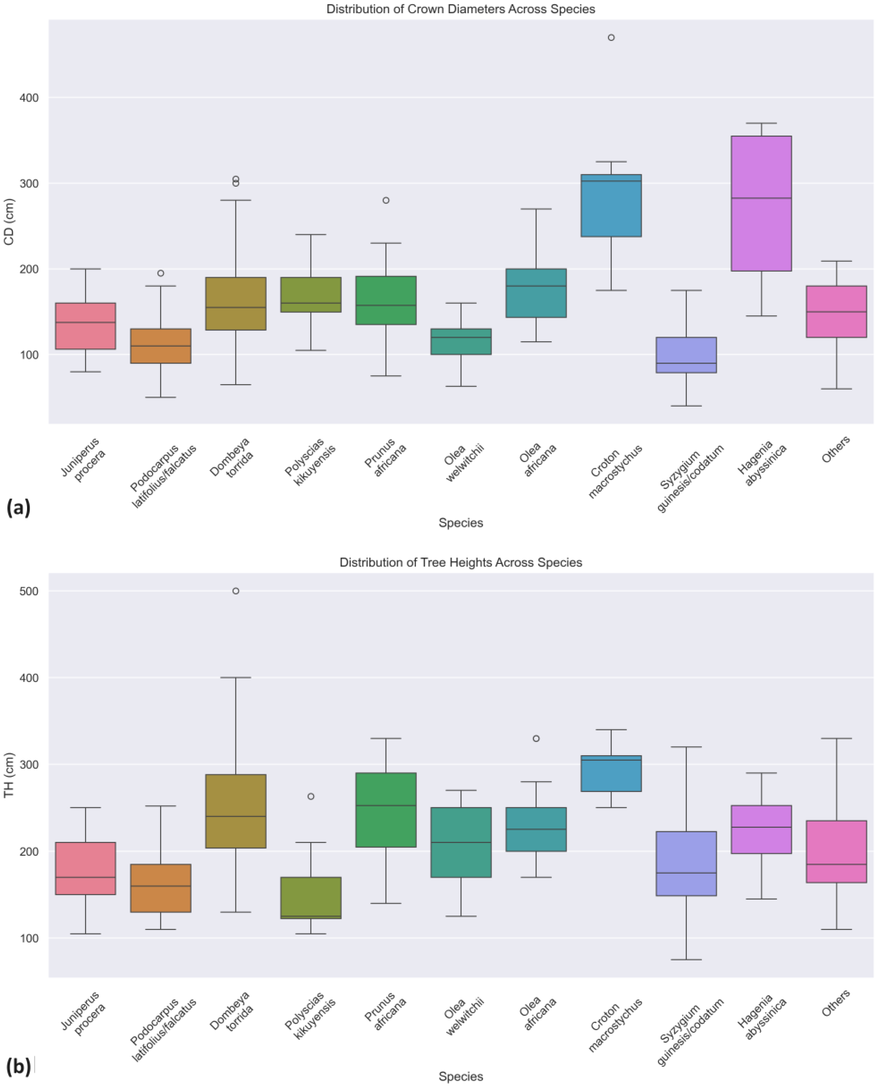
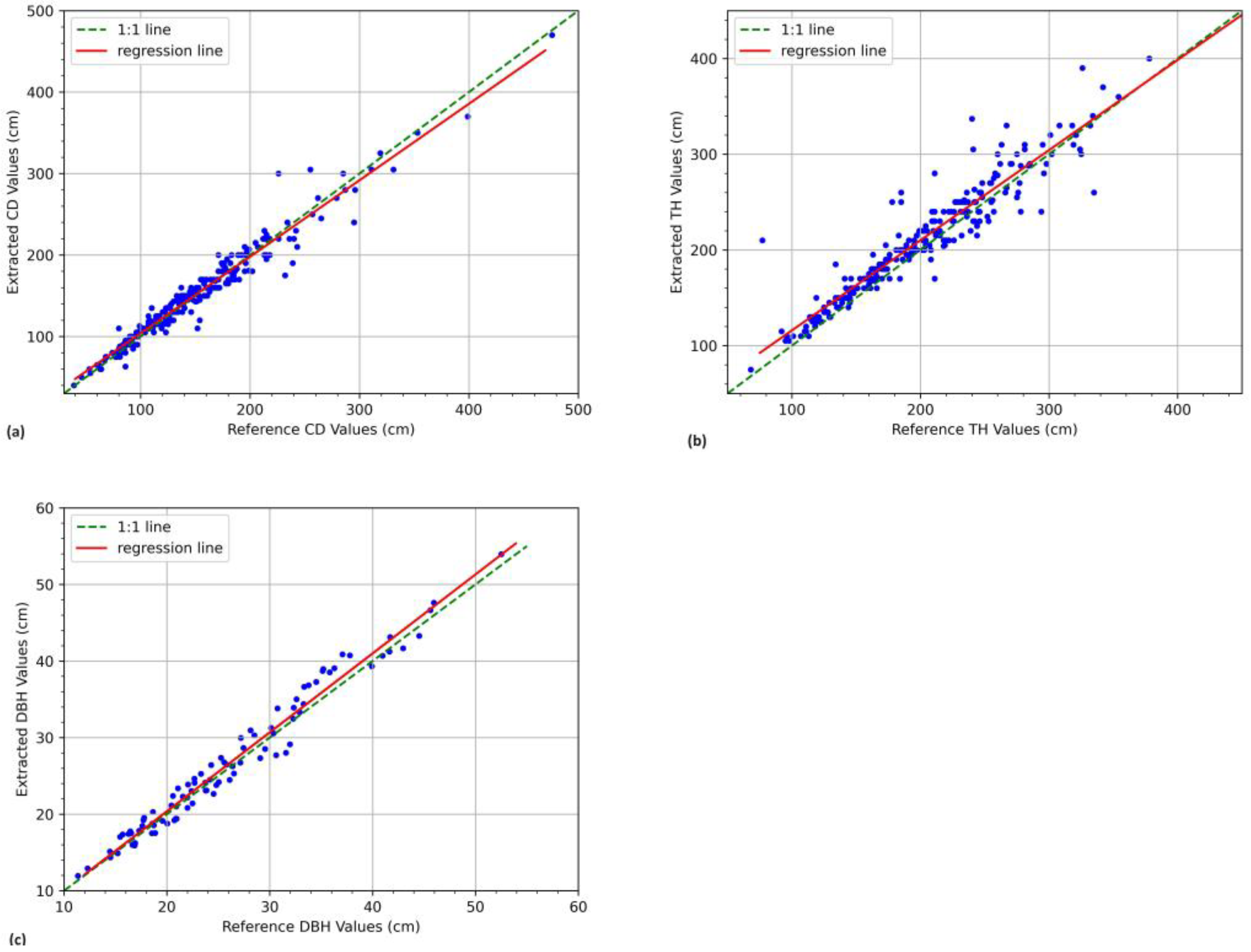
This study demonstrated stereoscopic photogrammetry for estimating tree measurements in a recently planted stand. Overall, we found that this method of non-contact tree inventory yields measurements that closely approximate ground truth measurements, as seen by the high accuracies reported. The mean absolute percentage errors (MAPEs) for the CDs, THs, and DBHs relative to the ground truth values were comparable, with slightly higher values for the tree heights. This may be attributed to the difficulty of achieving tree base delineation in images due to undergrowth and crops obstructing the view in the plantations. Similar challenges in tree extent delineation have been reported in previous studies involving non-contact techniques [52,68,83]. These same reasons may have also led to the greater underestimation of tree heights compared to crown diameters, as shown by the larger bias values. As such, it is worth pointing out that this technique is suited for use in sparse plantations where individual tree extent delineation in images is not difficult to achieve.
For all biophysical parameters, the correlation between estimated and ground truth values was very high, as indicated by the values of R 2 and the regression line slope, which are both very close to unity. Although similarly good results have been reported in other studies [57,59,64,67,68,73,84], this study is the first to present an extensive validation and analysis of the use of stereoscopic photogrammetry for tree parameter estimation in a real forest setting. The scattering profiles represent the variability in the individual measurements around the regression line. In the case of both parameters, the linear scattering profile situated close to the regression line coupled with the low MAPE values attest to the precision and reliability of our stereoscopic photogrammetry approach. Scatter plots and the other metrics reported here are highly recommended for gauging the performance of a method in biophysical parameter estimation [82]. Since the technique requires accurate segmentation of the tree to register good performance, the results affirm its practical significance in providing accurate estimates even in spatially heterogeneous environments. These findings have broader implications for forest monitoring practices, suggesting the method’s potential applicability and reliability in similar spatial contexts. Researchers and practitioners engaged in tree dimension estimation can leverage these insights to enhance their understanding and implementation of stereoscopic photogrammetry. In the broader context of planetary health, these parameters may then be used as input variables to allometric equations for calculating biomass and carbon stocks, for developing tree growth models, and so on [11,21,85].
As shown in Table A2 (Appendix B), the acquisition and storage of an image pair take place instantly since the actions themselves involve nothing more than capturing images. Since the processing of the images is performed after the acquisition is completed, the images of all the sampled trees can be acquired in the field, making the field survey exercise much faster and less cumbersome. Segmentation of the images in this study involved significant human interaction using image labelling software to ensure perfectly accurate masks were generated. This step can, however, be automated by implementing semantic segmentation based on deep learning [86,
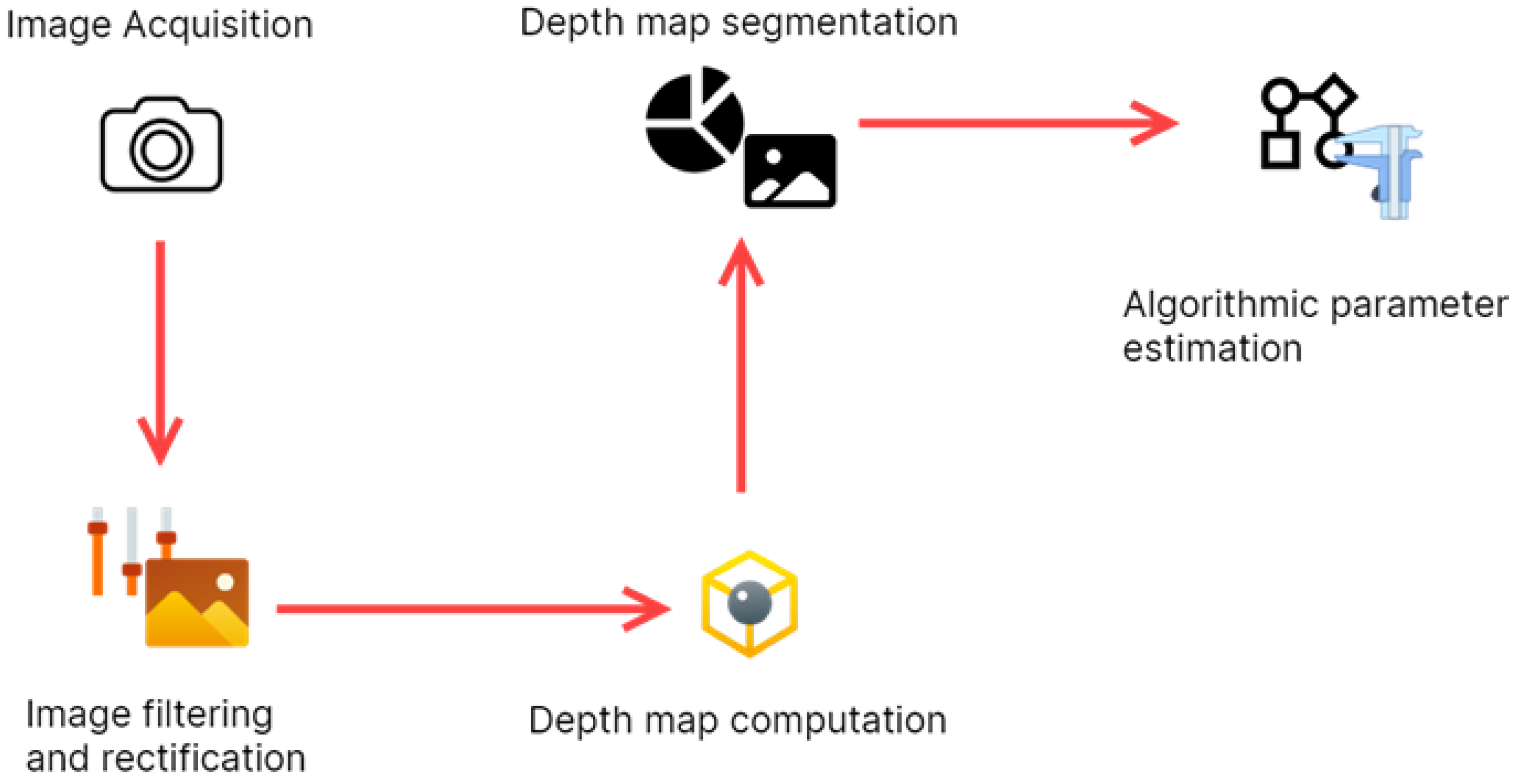
87], thus paving the way for real-time tree parameter estimation. This is an area of investigation for future research. The rest of the steps of image filtering, rectification, depth map computation and segmentation, and algorithmic parameter estimation are all packaged in a piece of software developed during this study [78]. Using this software, the extraction of all parameters of the 251 trees took approximately 2 min, a much shorter period than the three days taken to collect the ground truth data in the field. These observations imply that obtaining tree biophysical parameters from sample plots is much easier and faster using stereoscopic photogrammetry.
As an emerging proximate sensing technology, stereoscopic photogrammetry proves invaluable in field surveys and, consequently, in the effective implementation of REDD+. This technology facilitates the swift estimation of tree biophysical parameters, ensuring a rapid and efficient process [57,64,68,73]. Given that REDD+ and other policy frameworks necessitate precise data for informed decision making [3,4,6,10], the accuracy reported in this study underscores the potential of stereoscopic photogrammetry to contribute to evidence-based policy formulation. This aligns seamlessly with international reporting obligations, exemplified by the Global Forest Resources Assessment (FRA) [1,3,6,7], where the granularity of forest inventory data is an imperative commitment fulfilled by this technique [20]. The minimal training required for its use further enhances the capacity of forest management agencies to implement comprehensive forest-related policies.
Comprehensive and meticulous records of above-ground biomass (AGB) in Kenya are notably scarce [25,26], a common challenge facing many developing nations where the availability of high-quality data for international reporting lags behind that of developed counterparts [3]. Addressing these issues necessitates the establishment of a robust national forest monitoring system (a plan that is underway in Kenya) that would provide a dependable framework for forest monitoring [3,5,40]. As an emerging plot-level forest inventory technology, stereoscopic photogrammetry seamlessly aligns with this objective, offering precise measurements that increase the accuracy of carbon sequestration assessments [17]. Beyond carbon estimation, the proposed technique proves invaluable for monitoring reforestation and afforestation initiatives by enabling the timely tracking of stand growth in rapidly developing plantations such as young forest stands [39]. This becomes particularly pivotal in areas witnessing extensive reforestation and afforestation, where the monitoring rate needs to keep up with the pace of plantation establishment.
Since forests play a crucial role in carbon sequestration and climate change mitigation, there is a pressing need to consistently enhance the capacity for swift and precise forest monitoring. This study signifies a notable stride in that direction, constituting a valuable contribution toward the realisation of SDG 13 on climate action. The accuracy of projections aimed at reversing or mitigating climate change is intrinsically linked to the precision and reliability of the underlying data [11,21,69]. This underscores the importance of obtaining accurate data, a principle fundamental to this study. Moreover, the research aligns harmoniously with SDG 15 on biodiversity conservation, as it facilitates the monitoring of forest ecosystems, thereby contributing significantly to the preservation of biodiversity and the promotion of sustainable land management practices [30,31,38,77].
The cameras used in this study have a low resolution of 720 × 1280 pixels, which reduces the maximum distance from the stereo camera for which an accurate measurement can be extracted [48,49]. This is one of the limitations of this study and can be easily addressed by using higher-resolution cameras. In this study, we focused on estimating only the crown diameters and tree heights because the study area comprised mainly saplings with trunks covered by twigs or too slender to be measured. The occlusion of the trunk made it impossible to estimate the diameter using the proposed non-contact technique. This is yet another limitation of this technique and, indeed, an inherent limitation of light-based measurement systems [67,72]. Notwithstanding these limitations, the ability to extract the crown diameter and tree height in a fast, accurate, and low-cost non-contact approach as achieved in this study is a valuable contribution to the science of forest inventory, especially when monitoring young stands such as those in the study area.
Future research can be explored in areas such as automated tree crown segmentation based on deep learning, real-time biophysical parameter extraction, and the combination of terrestrial field surveys with aerial surveys for further validation.

5. Conclusions

This study successfully evaluated the applicability of stereoscopic photogrammetry for performing tree inventory of a recently reforested stand in Kenya. The need to monitor young stands is rising as reforestation efforts ramp up because of the government’s focus on climate change mitigation. Part of the country’s strategy is to establish a national forest monitoring system. This goal will require concerted efforts from the government, environmental agencies such as the Kenya Forestry Service, and universities. This study aligns with the government’s objective of building capacity for monitoring forests and implementing its REDD+ strategy. In this study, heights, crown diameters, and diameters at breast height of trees were estimated faster, more efficiently, and with reasonable accuracy, thus paving the way for quicker and more reliable estimation of biomass of carbon stocks. Through faster and more efficient methods for measuring these tree attributes, it will be possible to keep growing the national tree cover without losing track of the progress of already planted forests. Globally, this study contributes to planetary health and the United Nations’ SDGs 13 and 15 on climate action and biodiversity conservation, respectively.

Author Contributions

Conceptualisation, C.w.M. and B.O.; methodology, C.K.; software, C.K.; formal analysis, C.K.; investigation, C.K.; writing—original draft preparation, C.K.; writing—review and editing, C.w.M. and B.O.; supervision, C.w.M. and B.O.; project administration, C.w.M.; resources, C.w.M.; funding acquisition, C.K. and C.w.M. All authors have read and agreed to the published version of the manuscript.

Funding

This work received funding from the Dedan Kimathi University of Technology. The Centre for Data Science and Artificial Intelligence (DSAIL) received a hardware grant from the NVIDIA Corporation. We also thank Safaricom PLC for funding DSAIL for the Integrated Forest Monitoring project.

Data Availability Statement

The data that support the findings of this study, as well as the software code, are publicly available on GitHub: https://github.com/DeKUT-DSAIL/TreeVision (accessed on 11 August 2023).

Acknowledgments

We would like to thank the Kenya Forestry Service for granting access to the study area and their personnel for assisting us during the field data collection.

Conflicts of Interest

The authors declare that they have no known competing financial interests or personal relationships that could have appeared to influence the work reported in this paper. Billy Okal is employee of NVIDIA Corporation, Safaricom PLC and NVIDIA Corporation provided funding and teachnical support for the work. The funder had no role in the design of the study; in the collection, analysis, or interpretation of data, in the writing of the manuscript, or in the decision to publish the results.

Appendix A. Materials and Methods

Appendix A.1. Cost of Materials

A breakdown of the cost of the acquisition setup is provided in Table A1. On an item-by-item comparison, the amount we spent is lower compared to that spent in the studies of Eliopoulos et al. [16] and McGlade et al. [32], who spent USD 179 and USD 399 on the depth cameras alone and are both described as using low-cost approaches.
Table A1. Material cost breakdown.
ItemQtyCost (KES)Cost (USD)
Logitech C270 720p USB camera210,000.0071.00
3D-printed stereo camera rig15500.0039.00
NVIDIA Jetson Nano 2GB Developer Kit121,000.00149.00
7-inch HDMI LCD 1024 × 600 screen112,500.0090.00
20,000 mAh Oraimo power bank13000.0021.00
Total 52,000.00370.00

Appendix A.2. Geometry Derivation

The algorithm for extracting the three parameters of interest relies heavily on the scene geometry and camera specifications. In the figures presented in the following sections, the real-world distances between the stereo camera and various points on the tree are derived from the disparity images.

Appendix A.2.1. Estimating the Breast Height

The geometry for locating the breast height in a disparity image is shown in Figure A1.
Figure A1. Geometry for estimating BH location.
Challenges 15 00016 g0a1
Using Equation (A1), the coordinates of the trunk base b are found as ( x b ,   y b ,   z b ) . The angle β is calculated using trigonometry as follows:
β = tan 1 z b y b
The cosine rule is applied as follows:
d h 2 = h f 2 + d g 2 2 h f d g cos β = 1.3 2 + d g 2 2.6 d g cos β
where h f 1.3   m is approximately the breast height (1.3 m above the ground).
d g = x b 2 + y b 2 + z b 2
d h = 1.69 + d g 2 2.6 d g cos β
The sine rule is used as follows:
θ = sin 1 1.3 sin β d h
The camera has a vertical field of view v F o V = 28.68 ° :
s h p x = 720 × tan θ 2   tan v F o V 2 = 720 × tan θ 2   tan 14.31 = 2822.61 tan θ 2   p x
This is the number of pixels from the trunk base to the breast height.

Appendix A.2.2. Estimating the DBH

The geometry for estimating the DBH is obtained from Figure A2.
Figure A2. Geometry for estimating DBH.
Challenges 15 00016 g0a2
The horizontal field of view of the camera is h F o V = 48.81 ° . The DBH spans s d pixels in the disparity image. Therefore, the following is true:
1280   p x tan h F o V 2 = s d   p x tan θ
θ = tan 1 s d × 3.546 × 10 4
d a is obtained by converting the disparity of A to distance.
R = d a tan θ
D B H = 2 R
Figure A2 and the approach presented above were also used to calculate the crown diameter.

Appendix A.2.3. TH Estimation

To estimate the TH, Figure A3 is used.
Figure A3. Geometry for estimating TH.
Challenges 15 00016 g0a3
The lengths d T and d B are determined by finding the coordinates of points T and B, respectively, and calculating their respective distances from the camera. The following is then true:
720 tan 14.31 = s t   p x tan θ 2
θ 2 = tan 1 s t tan 14.31 720     θ = 2 × tan 1 s t × 3.543 × 10 4
ϕ = tan 1 z B y B
T B = T H = d T sin θ sin ϕ

Appendix A.3. Extraction Algorithms

Based on the scene geometry presented, we wrote computational geometric algorithms to extract the DBH, CD, and TH from the disparity maps.

Appendix A.3.1. Algorithm for Pixel of Interest Identification

AlgorithmA1
InputLeft and right images, mask, calibration parameters
OutputVector of intensities of pixels of interest
Step 1Compute disparity image
Step 2Mask the disparity image
Step 3Find the non-zero pixels in the masked disparity image
Step 4Calculate the row of the breast height
Step 5Identify the base, breast height, top, and crown regions of interest
Step 6Find median intensities in all regions of interest (base, breast height, top, and crown
Step 7Save intensities in a vector

Appendix A.3.2. Algorithm for DBH Extraction

AlgorithmA2
InputLeft and right images, mask, calibration parameters, reference DBH
OutputDBH value, error in estimation
Step 1Compute disparity image
Step 2Mask the disparity image
Step 3Find the non-zero pixels in the masked disparity image
Step 4Calculate the row of the breast height
Step 5Identify the base and breast height regions of interest
Step 6Find median intensities in base ( b ) and breast height ( h ) regions of interest
Step 7 Find   coordinates   of   b = x b , y b , z b   and   distance   to   b as d b = x b 2 + y b 2 + z b 2
Step 8 Find   coordinates   of   x = ( x h , y h , z h )   and   distance   to   h   as   d b = x h 2 + y h 2 + z h 2
Step 9 Find   angle   θ 1 subtended by breast height at the camera
Step 10Find number of non-zero pixels at the breast height
Step 11 Find   angle   θ 2 subtended by breast height at the camera
Step 12 Calculate   DBH   from   θ 2   and   d a , and compute error in estimation

Appendix A.3.3. Algorithm for TH Extraction

AlgorithmA3
InputLeft and right images, mask, calibration parameters, reference TH
OutputTH value, error in estimation
Step 1Compute disparity image
Step 2Mask the disparity image
Step 3Find the non-zero pixels in the masked disparity image
Step 4Identify the base and top regions of interest
Step 5Find median intensities in base ( b ) and top ( t ) regions of interest
Step 6Find coordinates of b as ( x b , y b , z b ) and distance to b as d b = x b 2 + y b 2 + z b 2
Step 7Find coordinates of t as ( x h , y h , z h ) and distance to t as d t = x t 2 + y t 2 + z t 2
Step 8 Find   complementary   of   angle   ϕ subtended at tree base by camera height
Step 10 Find   angle   θ subtended by tree height at the camera
Step 11 Find   angle   θ 2 subtended by breast height at the camera
Step 12 Calculate   TH   from   θ ϕ ,   and   d t , and compute error in estimation

Appendix A.3.4. Algorithm for CD Extraction

AlgorithmA4
InputLeft and right images, mask, calibration parameters, reference TH
OutputTH value, error in estimation
Step 1Compute disparity image
Step 2Mask the disparity image
Step 3Find the non-zero pixels in the masked disparity image
Step 4Identify the crown region of interest
Step 5Find median intensities in the crown ( c ) regions of interest
Step 6 Find   coordinates   of   c   as   ( x c , y c , z c )   and   distance   to   c   as   d c = x c 2 + y c 2 + z c 2
Step 7Find angle θ subtended by the crown at the camera
Step 8Calculate CD from θ and d c , and compute error in estimation

Appendix A.4. Camera Calibration and Depth Map Generation

Camera calibration was performed using OpenCV’s implementation of Zhang’s algorithm [88] to estimate the camera’s intrinsic and extrinsic parameters. These parameters were used to compute the image rectification and undistortion transformation mappings. This was done by capturing 30 images of a 6 × 9 checkerboard pattern and using OpenCV functions to extract these parameters.
Stereo matching between the left and right images was performed using OpenCV’s implementation of the Semi-Global Block Matching (SGBM) algorithm, a modified version of Hirschmuller’s Semi-Global Matching (SGM) technique [66]. The disparities in SGM are computed based on information contained in neighbouring pixels in eight directions. To reduce computational complexity, SGBM matches blocks rather than pixels, allowing for matching cost aggregation from five and eight directions instead of only eight. Post-processing steps applied to the resulting disparity image include peak removal by invalidating small segments, image normalisation to fit the intensities within the range 0 to 255, and median filtering to remove other irregularities.

Appendix A.5. Distance–Disparity Relationship

An accurate distance estimation using the disparity map established a consistent relationship between distance and disparity. Disparity maps for a single tree were computed from image pairs taken in the range of 3.0 m to 12.6 m from the trunk. The disparities of the trunk’s mid-point in the middle row of the disparity map were recorded. A distance–disparity scatter plot was then obtained followed by curve fitting using the Trust-Region-Reflective Least Squares optimisation [89] available on MATLAB. From two-view geometry, the depth of a point on the scene varies inversely to its disparity. In fitting the curve, this was taken into consideration and the best resulting curve was a rational polynomial with a numerator of order 2 and a denominator of order 3. Equation (A2) represents the curve, with x being the pixel intensity and y the distance in metres.
y = 346 x 2 116.7 x 1.961 x 3 5.863 x 2 + 47.24 x + 487.6
Given a disparity image D m with the left image as the base, the real-world coordinates of any pixel p on the image in the camera coordinate frame are the vector given by Equation (A3).
x b y b z b = b u l u r u l v l f x o x o y 0
where u l and v l are the x and y ordinates of the pixel p in the disparity image, o x ,   o y is the principal point of the image, f x is the focal length of the camera along the x direction in pixels, and u l u r is the disparity of the point at pixel p . The value u l a l s o   e q u a l s the greyscale intensity of pixel p in the disparity map.

Appendix A.6. Finding the Pixels of Interest

The pixels of interest are the edge pixels at the tree’s base, top, crown extremes, and breast height. The pixels of interest for TH and CD estimation are the easiest to locate since they are simply the top, base, and crown edge pixels, respectively. In the case of the DBH, the method presented for locating the breast height will be applied and edge pixels at that height will subsequently be identified. In a good disparity image, the pixels of interest have greyscale intensity values equal to or close to those pixels in their neighbourhood. However, there may be anomalies (sharp changes in pixel intensities) in some cases. Since the real-world distance to a pixel is based on its greyscale intensity, anomalies can cause errors in distance estimation and parameter extraction.
To eliminate the effect of these anomalies, regions of interest are formed from sets of pixels surrounding the pixels of interest (Figure A4). In the case of base and top pixels, the region of interest includes all pixels in the bottom 20 rows and the top 20 rows of the object pixels in the disparity map. In the case of the DBH, all non-zero pixels five rows above and five rows below the breast height location constitute the region of interest. The disparity of the pixel of interest is taken as the median of pixel intensities in the region of interest.
Figure A4. Forming regions of interest.
Challenges 15 00016 g0a4

Appendix B. Results

Image Acquisition and Processing Times

Table A2 shows a breakdown of the time taken to acquire and process each image pair until the tree parameters are obtained algorithmically. The total time taken to extract the crown diameters and tree heights of the 251 trees and the DBH from the 90 trees is included in the table.
Table A2. Image acquisition and processing times.
ActivityTime Taken
Image acquisition (per image pair)<1 s
Depth map computation (per image pair): filtering, rectification, correspondence matching, post-processing, masking3.1 s
Image segmentation (per image)2 min
TH and CD extraction (per depth map)<1 s
TH and CD extraction (251 depth maps)2 min
DBH extraction (per depth map)<1 s
DBH extraction (251 depth maps)<1 min

References

  1. FAO. Global Forest Resources Assessment 2020; FAO: Rome, Italy, 2020. [Google Scholar] [CrossRef]
  2. Hu, T.; Su, Y.; Xue, B.; Liu, J.; Zhao, X.; Fang, J.; Guo, Q. Mapping Global Forest Aboveground Biomass with Spaceborne LiDAR, Optical Imagery, and Forest Inventory Data. Remote Sens. 2016, 8, 565. [Google Scholar] [CrossRef]
  3. Nesha, K.; Herold, M.; De Sy, V.; Duchelle, A.E.; Martius, C.; Branthomme, A.; Garzuglia, M.; Jonsson, O.; Pekkarinen, A. An assessment of data sources, data quality and changes in national forest monitoring capacities in the Global Forest Resources Assessment 2005–2020. Environ. Res. Lett. 2021, 16, 54029. [Google Scholar] [CrossRef]
  4. von Gadow, K.; Zhang, C.Y.; Zhao, X.H. Science-based forest design. Math. Comput. For. Nat. Resour. Sci. MCFNS 2009, 1, 14–25. Available online: https://mcfns.net/index.php/Journal/article/view/MCFNS.1-14/46 (accessed on 21 October 2022).
  5. Smith, W. Forest inventory and analysis: A national inventory and monitoring program. Environ. Pollut. 2002, 116, S233–S242. [Google Scholar] [CrossRef]
  6. Keenan, R.J.; Reams, G.A.; Achard, F.; de Freitas, J.V.; Grainger, A.; Lindquist, E. Dynamics of global forest area: Results from the FAO Global Forest Resources Assessment 2015. For. Ecol. Manag. 2015, 352, 9–20. [Google Scholar] [CrossRef]
  7. MacDicken, K.G. Global Forest Resources Assessment 2015: What, why and how? For. Ecol. Manag. 2015, 352, 3–8. [Google Scholar] [CrossRef]
  8. Trumbore, S.; Brando, P.; Hartmann, H. Forest health and global change. Science 2015, 349, 814–818. [Google Scholar] [CrossRef]
  9. Bayati, H.; Najafi, A.; Vahidi, J.; Gholamali Jalali, S. 3D reconstruction of uneven-aged forest in single tree scale using digital camera and SfM-MVS technique. Scand. J. For. Res. 2021, 36, 210–220. [Google Scholar] [CrossRef]
  10. Breidenbach, J.; McRoberts, R.E.; Alberdi, I.; Antón-Fernández, C.; Tomppo, E. A century of national forest inventories—Informing past, present and future decisions. For. Ecosyst. 2020, 8, 36. [Google Scholar] [CrossRef]
  11. Jones, A.R.; Raja Segaran, R.; Clarke, K.D.; Waycott, M.; Goh, W.S.H.; Gillanders, B.M. Estimating Mangrove Tree Biomass and Carbon Content: A Comparison of Forest Inventory Techniques and Drone Imagery. Front. Mar. Sci. 2020, 6, 784. [Google Scholar] [CrossRef]
  12. dos Santos, L.M.; Ferraz, G.A.e.S.; Barbosa, B.D.d.S.; Diotto, A.V.; Maciel, D.T.; Xavier, L.A.G. Biophysical parameters of coffee crop estimated by UAV RGB images. Precis. Agric. 2020, 21, 1227–1241. [Google Scholar] [CrossRef]
  13. Santoro, M.; Cartus, O.; Carvalhais, N.; Rozendaal, D.M.A.; Avitabile, V.; Araza, A.; de Bruin, S.; Herold, M.; Quegan, S.; Rodríguez-Veiga, P.; et al. The global forest above-ground biomass pool for 2010 estimated from high-resolution satellite observations. Earth Syst. Sci. Data 2021, 13, 3927–3950. [Google Scholar] [CrossRef]
  14. Spawn, S.A.; Sullivan, C.C.; Lark, T.J.; Gibbs, H.K. Harmonized global maps of above and belowground biomass carbon density in the year 2010. Sci. Data 2020, 7, 122. [Google Scholar] [CrossRef] [PubMed]
  15. Reiersen, G.; Dao, D.; Lütjens, B.; Klemmer, K.; Amara, K.; Steinegger, A.; Zhang, C.; Zhu, X. ReforesTree: A Dataset for Estimating Tropical Forest Carbon Stock with Deep Learning and Aerial Imagery. In Proceedings of the AAAI Conference on Artificial Intelligence, Online, 22 February–1 March 2022; Volume 36, pp. 12119–12125. [Google Scholar] [CrossRef]
  16. Fassnacht, F.E.; Latifi, H.; Stereńczak, K.; Modzelewska, A.; Lefsky, M.; Waser, L.T.; Straub, C.; Ghosh, A. Review of studies on tree species classification from remotely sensed data. Remote Sens. Environ. 2016, 186, 64–87. [Google Scholar] [CrossRef]
  17. Fassnacht, F.E.; White, J.C.; Wulder, M.A.; Næsset, E. Remote sensing in forestry: Current challenges, considerations and directions. For. Int. J. For. Res. 2023, 97, 11–37. [Google Scholar] [CrossRef]
  18. Showstack, R. Global Forest Watch Initiative Provides Opportunity for Worldwide Monitoring. EOS Trans. Am. Geophys. Union 2014, 95, 77–79. [Google Scholar] [CrossRef]
  19. Næsset, E. Area-Based Inventory in Norway—From Innovation to an Operational Reality. In Forestry Applications of Airborne Laser Scanning: Concepts and Case Studies; Springer: Dordrecht, The Netherlands, 2014; pp. 215–240. [Google Scholar] [CrossRef]
  20. Lei, X.; Tang, M.; Lu, Y.; Hong, L.; Tian, D. Forest inventory in China: Status and challenges. Int. For. Rev. 2009, 11, 52–63. [Google Scholar] [CrossRef]
  21. Mutwiri, F.K.; Odera, P.A.; Kinyanjui, M.J. Estimation of Tree Height and Forest Biomass Using Airborne LiDAR Data: A Case Study of Londiani Forest Block in the Mau Complex, Kenya. Open J. For. 2017, 07, 255–269. [Google Scholar] [CrossRef]
  22. Neba, G. Assessment and Prediction of Above-Ground Biomass in Selectively Logged Forest Concessions Using Field Measurements and Remote Sensing Data: Case Study in Southeast Cameroon; University of Helsinki: Helsinki, Finland, 2013. [Google Scholar] [CrossRef]
  23. Natarajan, K.; Latva-Käyrä, P.; Zyadin, A.; Chauhan, S.; Singh, H.; Pappinen, A.; Pelkonen, P. Biomass Resource Assessment and Existing Biomass Use in the Madhya Pradesh, Maharashtra, and Tamil Nadu States of India. Challenges 2015, 6, 158–172. [Google Scholar] [CrossRef]
  24. Halder, P.; Arevalo, J.; Tahvanainen, L.; Pelkonen, P. Benefits and Challenges Associated with the Development of Forest-Based Bioenergy Projects in India: Results from an Expert Survey. Challenges 2014, 5, 100–111. [Google Scholar] [CrossRef]
  25. Rodríguez-Veiga, P.; Carreiras, J.; Smallman, T.L.; Exbrayat, J.-F.; Ndambiri, J.; Mutwiri, F.; Nyasaka, D.; Quegan, S.; Williams, M.; Balzter, H. Carbon Stocks and Fluxes in Kenyan Forests and Wooded Grasslands Derived from Earth Observation and Model-Data Fusion. Remote Sens. 2020, 12, 2380. [Google Scholar] [CrossRef]
  26. Nyamari, N.; Cabral, P. Impact of land cover changes on carbon stock trends in Kenya for spatial implementation of REDD+ policy. Appl. Geogr. 2021, 133, 102479. [Google Scholar] [CrossRef]
  27. Masayi, N.N.; Omondi, P.; Tsingalia, M. Assessment of land use and land cover changes in Kenya’s Mt. Elgon forest ecosystem. Afr. J. Ecol. 2021, 59, 988–1003. [Google Scholar] [CrossRef]
  28. Odawa, S.; Seo, Y. Water Tower Ecosystems under the Influence of Land Cover Change and Population Growth: Focus on Mau Water Tower in Kenya. Sustainability 2019, 11, 3524. [Google Scholar] [CrossRef]
  29. Kogo, B.K.; Kumar, L.; Koech, R. Analysis of spatio-temporal dynamics of land use and cover changes in Western Kenya. Geocarto Int. 2021, 36, 376–391. [Google Scholar] [CrossRef]
  30. Rotich, B.; Ojwang, D. Trends and drivers of forest cover change in the Cherangany hills forest ecosystem, western Kenya. Glob. Ecol. Conserv. 2021, 30, e01755. [Google Scholar] [CrossRef]
  31. Kibetu, K.; Mwangi, M. Assessment of Forest Rehabilitation and Restocking Along Mt. Kenya East Forest Reserve Using Remote Sensing Data. Afr. J. Sci. Technol. Eng. 2020, 1, 113–126. [Google Scholar]
  32. Ngigi, T.G.; Tateishi, R. Monitoring deforestation in Kenya. Int. J. Environ. Stud. 2004, 61, 281–291. [Google Scholar] [CrossRef]
  33. Mwangi, N.; Waithaka, H.; Mundia, C.; Kinyanjui, M.; Mutua, F. Assessment of drivers of forest changes using multi-temporal analysis and boosted regression trees model: A case study of Nyeri County, Central Region of Kenya. Model. Earth Syst. Environ. 2020, 6, 1657–1670. [Google Scholar] [CrossRef]
  34. Kogo, B.K.; Kumar, L.; Koech, R. Forest cover dynamics and underlying driving forces affecting ecosystem services in western Kenya. Remote Sens. Appl. 2019, 14, 75–83. [Google Scholar] [CrossRef]
  35. Kairo, J.; Mbatha, A.; Murithi, M.M.; Mungai, F. Total Ecosystem Carbon Stocks of Mangroves in Lamu, Kenya; and Their Potential Contributions to the Climate Change Agenda in the Country. Front. For. Glob. Chang. 2021, 4, 709227. [Google Scholar] [CrossRef]
  36. Elizabeth, W.W.; Gilbert, O.O.; Bernard, K.K. Effect of forest management approach on household economy and community participation in conservation: A case of Aberdare Forest Ecosystem, Kenya. Int. J. Biodivers. Conserv. 2018, 10, 172–184. [Google Scholar] [CrossRef]
  37. Okumu, B.; Muchapondwa, E. Welfare and forest cover impacts of incentive based conservation: Evidence from Kenyan community forest associations. World Dev. 2020, 129, 104890. [Google Scholar] [CrossRef]
  38. Kilonzi, F.; Ota, T. Ecosystem service preferences across multilevel stakeholders in co-managed forests: Case of Aberdare protected forest ecosystem in Kenya. One Ecosyst. 2019, 4, e36768. [Google Scholar] [CrossRef]
  39. Eisen, N. Restoring the Commons: Joint Reforestation Governance in Kenya; Harvard University: Cambridge, MA, USA, 2019. [Google Scholar]
  40. Ministry of Environment and Forestry. The National Forest Reference Level for REDD+ Implementation; Ministry of Environment and Forestry: New Delhi, India, 2020.
  41. Klopp, J.M. Deforestation and democratization: Patronage, politics and forests in Kenya. J. East. Afr. Stud. 2012, 6, 351–370. [Google Scholar] [CrossRef]
  42. Fernandes, G.W.; Coelho, M.S.; Machado, R.B.; Ferreira, M.E.; Aguiar, L.M.d.S.; Dirzo, R.; Scariot, A.; Lopes, C.R. Afforestation of savannas: An impending ecological disaster. Perspect. Ecol. Conserv. 2016, 14, 146–151. [Google Scholar] [CrossRef]
  43. Ministry of Environment and Forestry. National Strategy for Achieving and Maintaining over 10% Tree Cover by 2022 (2019–2022); Ministry of Environment and Forestry: Nairobi, Kenya, 2019.
  44. Cervantes, A.G.; Gutierrez, P.T.V.; Robinson, S.C. Forest Inventories in Private and Protected Areas of Paraguay. Challenges 2023, 14, 23. [Google Scholar] [CrossRef]
  45. Forsman, M.; Börlin, N.; Holmgren, J. Estimation of tree stem attributes using terrestrial photogrammetry with a camera rig. Forests 2016, 7, 61. [Google Scholar] [CrossRef]
  46. Otero, V.; Van De Kerchove, R.; Satyanarayana, B.; Martínez-Espinosa, C.; Fisol, M.A.B.; Ibrahim, M.R.B.; Sulong, I.; Mohd-Lokman, H.; Lucas, R.; Dahdouh-Guebas, F. Managing mangrove forests from the sky: Forest inventory using field data and Unmanned Aerial Vehicle (UAV) imagery in the Matang Mangrove Forest Reserve, peninsular Malaysia. For. Ecol. Manag. 2018, 411, 35–45. [Google Scholar] [CrossRef]
  47. Liang, X.; Jaakkola, A.; Wang, Y.; Hyyppä, J.; Honkavaara, E.; Liu, J.; Kaartinen, H. The Use of a Hand-Held Camera for Individual Tree 3D Mapping in Forest Sample Plots. Remote Sens. 2014, 6, 6587–6603. [Google Scholar] [CrossRef]
  48. Szeliski, R. Computer Vision: Algorithms and Applications; Springer: Dordrecht, The Netherlands, 2011. [Google Scholar] [CrossRef]
  49. Hartley, R.; Zisserman, A. Multiple View Geometry in Computer Vision, 2nd ed.; Cambridge University Press: Cambridge, UK, 2003. [Google Scholar] [CrossRef]
  50. Piermattei, L.; Karel, W.; Wang, D.; Wieser, M.; Mokroš, M.; Surový, P.; Koreň, M.; Tomaštík, J.; Pfeifer, N.; Hollaus, M. Terrestrial Structure from Motion Photogrammetry for Deriving Forest Inventory Data. Remote Sens. 2019, 11, 950. [Google Scholar] [CrossRef]
  51. Puliti, S.; Solberg, S.; Granhus, A. Use of UAV Photogrammetric Data for Estimation of Biophysical Properties in Forest Stands Under Regeneration. Remote Sens. 2019, 11, 233. [Google Scholar] [CrossRef]
  52. Guerra-Hernández, J.; Cosenza, D.N.; Rodriguez, L.C.E.; Silva, M.; Tomé, M.; Díaz-Varela, R.A.; González-Ferreiro, E. Comparison of ALS- and UAV(SfM)-derived high-density point clouds for individual tree detection in Eucalyptus plantations. Int. J. Remote Sens. 2018, 39, 5211–5235. [Google Scholar] [CrossRef]
  53. Collazos, D.T.; Cano, V.R.; Villota, J.C.P.; Toro, W.M. A photogrammetric system for dendrometric feature estimation of individual trees. In Proceedings of the 2018 IEEE 2nd Colombian Conference on Robotics and Automation (CCRA), Barranquilla, Colombia, 1–3 November 2018; pp. 1–6. [Google Scholar] [CrossRef]
  54. Han, D.; Wang, C. Tree height measurement based on image processing embedded in smart mobile phone. In Proceedings of the 2011 International Conference on Multimedia Technology, Hangzhou, China, 26–28 July 2011; pp. 3293–3296. [Google Scholar] [CrossRef]
  55. Cabo, C.; Ordóñez, C.; López-Sánchez, C.A.; Armesto, J. Automatic dendrometry: Tree detection, tree height and diameter estimation using terrestrial laser scanning. Int. J. Appl. Earth Obs. Geoinf. 2018, 69, 164–174. [Google Scholar] [CrossRef]
  56. Corte, A.P.D.; Souza, D.V.; Rex, F.E.; Sanquetta, C.R.; Mohan, M.; Silva, C.A.; Zambrano, A.M.A.; Prata, G.; de Almeida, D.R.A.; Trautenmüller, J.W.; et al. Forest inventory with high-density UAV-Lidar: Machine learning approaches for predicting individual tree attributes. Comput. Electron. Agric. 2020, 179, 105815. [Google Scholar] [CrossRef]
  57. Trairattanapa, V.; Ravankar, A.A.; Emaru, T. Estimation of Tree Diameter at Breast Height using Stereo Camera by Drone Surveying and Mobile Scanning Methods. In Proceedings of the 2020 59th Annual Conference of the Society of Instrument and Control Engineers of Japan (SICE), Chiang Mai, Thailand, 23–26 September 2020; pp. 946–951. [Google Scholar] [CrossRef]
  58. Marzulli, M.I.; Raumonen, P.; Greco, R.; Persia, M.; Tartarino, P. Estimating tree stem diameters and volume from smartphone photogrammetric point clouds. For. Int. J. For. Res. 2020, 93, 411–429. [Google Scholar] [CrossRef]
  59. St-Onge, B.; Vega, C.; Fournier, R.A.; Hu, Y. Mapping canopy height using a combination of digital stereo-photogrammetry and lidar. Int. J. Remote Sens. 2008, 29, 3343–3364. [Google Scholar] [CrossRef]
  60. Liu, L.; Zhang, A.; Xiao, S.; Hu, S.; He, N.; Pang, H.; Zhang, X.; Yang, S. Single Tree Segmentation and Diameter at Breast Height Estimation with Mobile LiDAR. IEEE Access 2021, 9, 24314–24325. [Google Scholar] [CrossRef]
  61. McGlade, J.; Wallace, L.; Hally, B.; White, A.; Reinke, K.; Jones, S. An early exploration of the use of the Microsoft Azure Kinect for estimation of urban tree Diameter at Breast Height. Remote Sens. Lett. 2020, 11, 963–972. [Google Scholar] [CrossRef]
  62. Fan, Y.; Feng, Z.; Mannan, A.; Khan, T.U.; Shen, C.; Saeed, S. Estimating Tree Position, Diameter at Breast Height, and Tree Height in Real-Time Using a Mobile Phone with RGB-D SLAM. Remote Sens. 2018, 10, 1845. [Google Scholar] [CrossRef]
  63. Chen, S.W.; Nardari, G.V.; Lee, E.S.; Qu, C.; Liu, X.; Romero, R.A.F.; Kumar, V. SLOAM: Semantic lidar odometry and mapping for forest inventory. IEEE Robot. Autom. Lett. 2020, 5, 612–619. [Google Scholar] [CrossRef]
  64. Eliopoulos, N.J.; Shen, Y.; Nguyen, M.L.; Arora, V.; Zhang, Y.; Shao, G.; Woeste, K.; Lu, Y.-H. Rapid Tree Diameter Computation with Terrestrial Stereoscopic Photogrammetry. J. For. 2020, 118, 355–361. [Google Scholar] [CrossRef]
  65. Aslam, A.; Ansari, M. Depth-map generation using pixel matching in stereoscopic pair of images. arXiv 2019, arXiv:1902.03471. [Google Scholar] [CrossRef]
  66. Hirschmuller, H. Stereo Processing by Semiglobal Matching and Mutual Information. IEEE Trans. Pattern Anal. Mach. Intell. 2007, 30, 328–341. [Google Scholar] [CrossRef]
  67. Perng, B.-H.; Lam, T.Y.; Lu, M.-K. Stereoscopic imaging with spherical panoramas for measuring tree distance and diameter under forest canopies. For. Int. J. For. Res. 2018, 91, 662–673. [Google Scholar] [CrossRef]
  68. Malekabadi, A.J.; Khojastehpour, M.; Emadi, B. Disparity map computation of tree using stereo vision system and effects of canopy shapes and foliage density. Comput. Electron. Agric. 2019, 156, 627–644. [Google Scholar] [CrossRef]
  69. Wang, Y.; Zhang, X.; Guo, Z. Estimation of tree height and aboveground biomass of coniferous forests in North China using stereo ZY-3, multispectral Sentinel-2, and DEM data. Ecol. Indic. 2021, 126, 107645. [Google Scholar] [CrossRef]
  70. Sánchez-González, M.; Cabrera, M.; Herrera, P.J.; Vallejo, R.; Cañellas, I.; Montes, F. Basal Area and Diameter Distribution Estimation Using Stereoscopic Hemispherical Images. Photogramm. Eng. Remote Sens. 2016, 82, 605–616. [Google Scholar] [CrossRef]
  71. Sun, C.; Jones, R.; Talbot, H.; Wu, X.; Cheong, K.; Beare, R.; Buckley, M.; Berman, M. Measuring the distance of vegetation from powerlines using stereo vision. ISPRS J. Photogramm. Remote Sens. 2006, 60, 269–283. [Google Scholar] [CrossRef]
  72. Wang, H.; Yang, T.-R.; Waldy, J.; Kershaw, J.A., Jr. Estimating Individual Tree Heights and DBHs From Vertically Displaced Spherical Image Pairs. Math. Comput. For. Nat. Resour. Sci. MCFNS 2021, 13, 1–14. Available online: http://mcfns.net/index.php/Journal/article/view/13.1/2021.1 (accessed on 20 July 2022).
  73. Malekabadi, A.J.; Khojastehpour, M. Optimization of stereo vision baseline and effects of canopy structure, pre-processing and imaging parameters for 3D reconstruction of trees. Mach. Vis. Appl. 2022, 33, 87. [Google Scholar] [CrossRef]
  74. Malekabadi, A.J.; Khojastehpour, M.; Emadi, B. Comparison of block-based stereo and semi-global algorithm and effects of pre-processing and imaging parameters on tree disparity map. Sci. Hortic. 2019, 247, 264–274. [Google Scholar] [CrossRef]
  75. Bayat, M.; Latifi, H.; Hosseininaveh, A. The architecture of a stereo image based system to measure tree geometric parameters. ISPRS Int. Arch. Photogramm. Remote Sens. Spat. Inf. Sci. 2019, 42, 183–189. [Google Scholar] [CrossRef]
  76. Nyukuri, J. Issues Influencing Sustainability of the Aberdare Range Forests: A Case of Kieni Forest in Gakoe Location, Kiambu County; University of Nairobi: Nairobi, Kenya, 2012. [Google Scholar]
  77. Kenya Forestry Service. Aberdare Forest Reserve Management Plan; Kenya Forestry Service: Nairobi, Kenya, 2010. [Google Scholar]
  78. Kiplimo, C.; Epege, C.E.; Maina, C.W.; Okal, B. DSAIL-TreeVision: A software tool for extracting tree biophysical parameters from stereoscopic images. SoftwareX 2024, 26, 101661. [Google Scholar] [CrossRef]
  79. Van Rossum, G.; Drake, F. Python Reference Manual; Python Software Foundation: Wilmington, DE, USA, 2001. [Google Scholar]
  80. Bradski, G. The OpenCV Library. Dr. Dobbs J. Softw. Tools 2000, 25, 120–126. Available online: https://www.drdobbs.com/open-source/the-opencv-library/184404319 (accessed on 22 December 2023).
  81. Virbel, M. Kivy Framework. 2022. Available online: https://github.com/kivy/kivy (accessed on 19 January 2024).
  82. Yin, D.; Wang, L. How to assess the accuracy of the individual tree-based forest inventory derived from remotely sensed data: A review. Int. J. Remote Sens. 2016, 37, 4521–4553. [Google Scholar] [CrossRef]
  83. Zhao, H.; Morgenroth, J.; Pearse, G.; Schindler, J. A Systematic Review of Individual Tree Crown Detection and Delineation with Convolutional Neural Networks (CNN). Curr. For. Rep. 2023, 9, 149–170. [Google Scholar] [CrossRef]
  84. Wang, B.H.; Diaz-Ruiz, C.; Banfi, J.; Campbell, M. Detecting and Mapping Trees in Unstructured Environments with a Stereo Camera and Pseudo-Lidar. In Proceedings of the 2021 IEEE International Conference on Robotics and Automation (ICRA), Xian, China, 30 May–5 June 2021; IEEE: New York, NY, USA, 2021; pp. 14120–14126. [Google Scholar] [CrossRef]
  85. Kinyanjui, M.J.; Latva-Käyrä, P.; Bhuwneshwar, P.S.; Kariuki, P.; Gichu, A.; Wamichwe, K. An Inventory of the Above Ground Biomass in the Mau Forest Ecosystem, Kenya. Open J. Ecol. 2014, 04, 619–627. [Google Scholar] [CrossRef]
  86. Jodas, D.S.; Brazolin, S.; Yojo, T.; de Lima, R.A.; Velasco, G.D.N.; Machado, A.R.; Papa, J.P. A Deep Learning-based Approach for Tree Trunk Segmentation. In Proceedings of the 2021 34th SIBGRAPI Conference on Graphics, Patterns, and Images (SIBGRAPI), Gramado, Brazil, 18–22 October 2021; pp. 370–377. [Google Scholar] [CrossRef]
  87. Grondin, V.; Fortin, J.-M.; Pomerleau, F.; Giguère, P. Tree detection and diameter estimation based on deep learning. For. Int. J. For. Res. 2023, 96, 264–276. [Google Scholar] [CrossRef]
  88. Zhang, Z. A flexible new technique for camera calibration. IEEE Trans. Pattern Anal. Mach. Intell. 2000, 22, 1330–1334. [Google Scholar] [CrossRef]
  89. Byrd, R.H.; Schnabel, R.B.; Shultz, G.A. Approximate solution of the trust region problem by minimization over two-dimensional subspaces. Math. Program. 1988, 40, 247–263. [Google Scholar] [CrossRef]
Figure 1. Study area in Kieni Forest.
Challenges 15 00016 g001
Figure 2. Workflow diagram.
Challenges 15 00016 g002
Figure 3. Images of the entire tree through the data processing pipeline.
Challenges 15 00016 g003
Figure 4. Distributions per species of crown diameters (a) and tree heights (b).
Challenges 15 00016 g004
Figure 5. Regression plots comparing reference and extracted (a) DBH values, (b) CD values, and (c) TH values.
Challenges 15 00016 g005
Table 1. Summary of performance evaluation results.
ParameterMAE (MAPE)BiasRMSE R 2 Slope
DBH1.41 cm (5.3%)−0.56 cm1.70 cm0.96501.0310
CD9.55 cm (6.43%)−0.96 cm13.37 cm0.94840.9385
TH15.78 cm (7.39%)−10.08 cm22.43 cm0.87080.9419
Disclaimer/Publisher’s Note: The statements, opinions and data contained in all publications are solely those of the individual author(s) and contributor(s) and not of MDPI and/or the editor(s). MDPI and/or the editor(s) disclaim responsibility for any injury to people or property resulting from any ideas, methods, instructions or products referred to in the content.

