Numerical Simulation of the Motion of a Large Scale Unmanned Surface Vessel in High Sea State Waves

Abstract

The motion stability of the Unmanned Surface Vessel (USV) is threatened by the action of waves under a rough sea state. In the present paper, the motion of a large-scale USV is numerically simulated under high sea state of level 5 and 7. The overset grid method and Reynolds Averaged Navier–Stokes (RANS) approach are employed to solve Navier–Stokes (N-S) equations. For the case of wave incident angle 0° and 30°, the heave, pitch and roll motion response of a large scale USV are investigated by using the six Degrees of Freedom (6-DOF) numerical model. The effects of different sea states, as well as different wave directions, on the motion of USV are compared. The comparative results indicate that the response of this USV in waves is the periodic free-motion according to the corresponding amplitude, which does not exceed the stable range, and there are no overturning and other situations that may affect the safety, in the case of level 5 and 7 sea states. The corresponding pressure at the bottom of this USV meets the range of material strength, and no structural damage or injury to the hull occurs, although the pressure varies at different wave periods. For the case of different wave directions, the analysis of the boundary layer thickness shows that the wave direction is of great importance to the boundary layer thickness distribution, both in the level 5 and level 7 sea states.

1. Introduction

In recent years, a variety of unmanned surface vehicles (USV) have emerged around the world for different operation requirements. As a new type of ocean carrying platform, USV is widely used in civil and military fields because of its small size, high mobility, intelligence, and all-weather operation. Spartan Scout of the United States, Silver Marlin of Israel, and Venus of Singapore have excellent performance in environmental monitoring, search and rescue activities, surveillance, and reconnaissance and patrol [1]. USV is becoming an important way to explore the ocean and an important tool for marine operations.

The motion response and resistance performance in a real sea state are very important for the safe and efficient completion of the task for USV. In real sea state, due to the interaction of waves, the resistance is larger than that in still water [2]. The maximum additional resistance of this part can reach 30% of the total resistance in still water [3]. At the same time, under the excitation of waves, the USV will produce obvious six degrees of freedom motion response [4], especially in high sea state, the excessive motion response will threaten its motion stability. The motion of ships in high sea states is related to the safety of navigation. Kim D. et al. [5] studied ship maneuverability under different wave conditions based on the CFD method. The main results of this study help to improve the understanding of ship maneuverability in waves, thus as to improve the safety of navigation. Jiri de Vos et al. [6] carried out statistical analysis on ship parameters of unmanned ship safely and obtained the length of an unmanned ship with maximum safety benefit. Chen et al. [7] did a detailed analysis of the relationship between ship responses and sea states under real rough sea conditions, which gives suggestions for ship safety under severe weather conditions. It is of great significance to study the hydrodynamic performance prediction of USV in high sea state for its shape design and hydrodynamic performance analysis.

Hydrodynamic prediction is an important basis for the performance research of USV. The common prediction methods include model experiments and numerical simulations. The model test has high reliability, but it needs a lot of time and money. Now it is mainly used as the final scheme verification and hydrodynamic mechanism research. Numerical simulation is widely used as the simplest and convenient method. The numerical methods for predicting ship motion response in waves include classical potential flow theory and unsteady Reynold’s time-averaged equations (RANS). Tarafder and Suzuki analyzed the free surface flow problem of Wigley catamaran based on the potential flow theory [8]. Based on the potential flow theory, Fang and Chan predicted the motion responses (including heave, pitch, and roll) of the Wave Piercing Catamaran (WPC) in regular and irregular waves. The numerical results are in good agreement with the experimental data obtained in SSPA [9]. Based on the linear potential flow theory, Ma and Wan studied the nonlinear effects of heave and trim motion, wave resistance of four buoyant hull types (Wigley, S60, DTMB5415, KCS) sailing in still water. The results show that the numerical prediction is consistent with the experimental results, and the nonlinear free surface will increase wave making [10]. Min Guk Seo and others used the Rankine panel method based on potential flow theory to calculate the resistance of KVLCC2 ship in short wave. It was found that when the face element scale was small enough, the additional resistance consistent with the experimental measurement could be accurately predicted [11]. In most of the numerical calculation methods, potential flow theory has high efficiency and accuracy under certain conditions, but the method based on potential flow theory also has some shortcomings. This method is mainly for medium speed design and does not consider the fluid viscosity. In the prediction of ship motion response, the influence of the viscosity effect cannot be ignored. Simonsen et al. also emphasized that the effects of breaking waves, turbulence, and viscosity, which are ignored in potential flow theory, should be taken into account in the numerical calculation [12]. RANS method based on CFD (Computational Fluid Dynamics) breaks through the limitation of potential flow theory and is more accurate in motion response and additional resistance prediction. Tahsin found that in the case of high-speed navigation, the additional resistance and motion response obtained by the RANS equation are most different from those based on potential flow theory [13]. Further comparison with the model experiment shows that the prediction results of RANS equation are more accurate. Deng Rui et al. studied the additional resistance and motion response of the trimaran under different wave amplitude conditions by using the method of viscosity based on RANS. The results show that the peak value of the additional resistance and motion response of the trimaran is mainly affected by the wavelength [14].

In this paper, a catamaran USV is taken as the research object, and the mesh is completed based on overlapping grid technology. The RANS method and SST k-ω are applied as the turbulent model to solve the N-S equation and simulates the motion of the USV in the high sea states of 5 and 7 levels. The motion response and resistance performance of the USV under high sea states are analyzed. The differences of the motion response under different wave directions are compared, and the hull pressure and boundary layer distribution under different working conditions are studied.

2. Numerical Model

2.1. Governing Equations and Turbulence Models

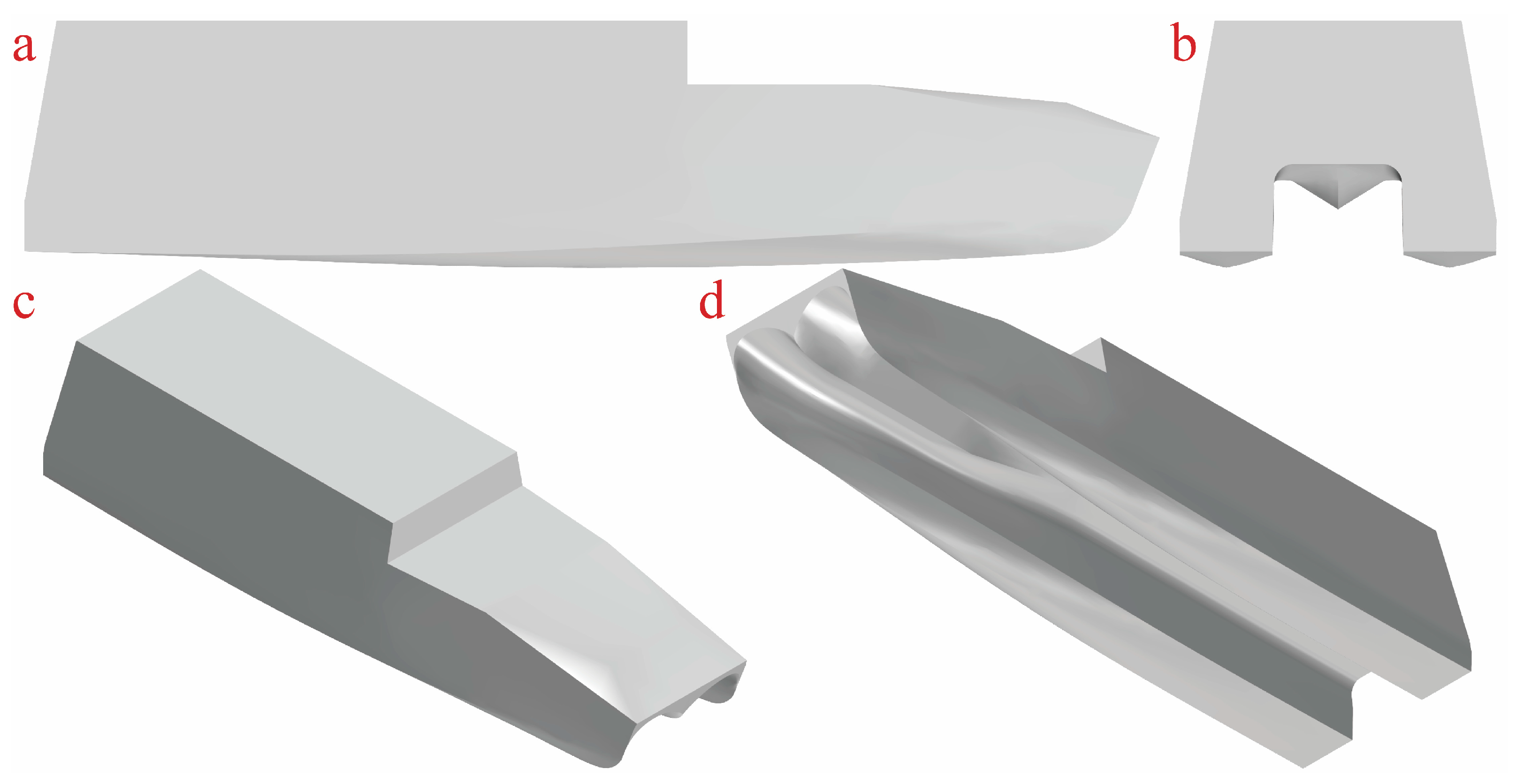
The RANS method was applied to solve the N-S equation in this paper, which avoids the huge amount of calculation caused by the direct simulation of turbulent pulsations at various scales. The continuity and momentum equations can be written in Cartesian coordinates as follows [15]:

$$\frac{\partial u_i}{\partial x_i}=0$$

(1)

$$\frac{\partial u_i}{\partial t}+\frac{\partial u_j{u}_i}{\partial x_j}=\frac{\partial }{\partial x_j}\mu (\frac{\partial u_i}{\partial x_j})-\frac{1}{\rho }\frac{\partial p}{\partial x_i}+S_j$$

(2)

where $u_i$ and $u_j$ ($i$, $j$ = 1, 2, 3), $p$, $\rho$, and $S_j$ represent the time-averaged values of velocity components, time-averaged pressure, fluid density, and source term, respectively. The fluid density was assumed constant for incompressible Newtonian fluids.

In this paper, The STAR-CCM+ commercial software package based on finite-volume computational method was used to analyze the interaction between USV and waves. The turbulence model used in this paper was the k-ω shear stress transport (SST) model [16]. The advantage of the SST k-ω turbulence model, compared with the standard k-ω model and k-ω model has higher accuracy and credibility. The free surface of the numerical wave tank was modeled using the two-phase volume-of-fluid (VOF) technique with the high-resolution interface capturing (HRIC) scheme [17].

2.2. USV Model

The calculation model is a full-scale model of a catamaran USV. The USV models from different perspectives are shown in Figure 1.

The detailed main parameters of the model are shown in

Table 1. Principal dimension of the USV.

Parameters	Symbol	Value
Length of overall (m)	LOA	42.00
Length between perpendiculars (m)	Lpp	41.05
Breadth (m)	B	12.00
Design draft (m)	T	1.45
Depth (m)	D	4.50

.

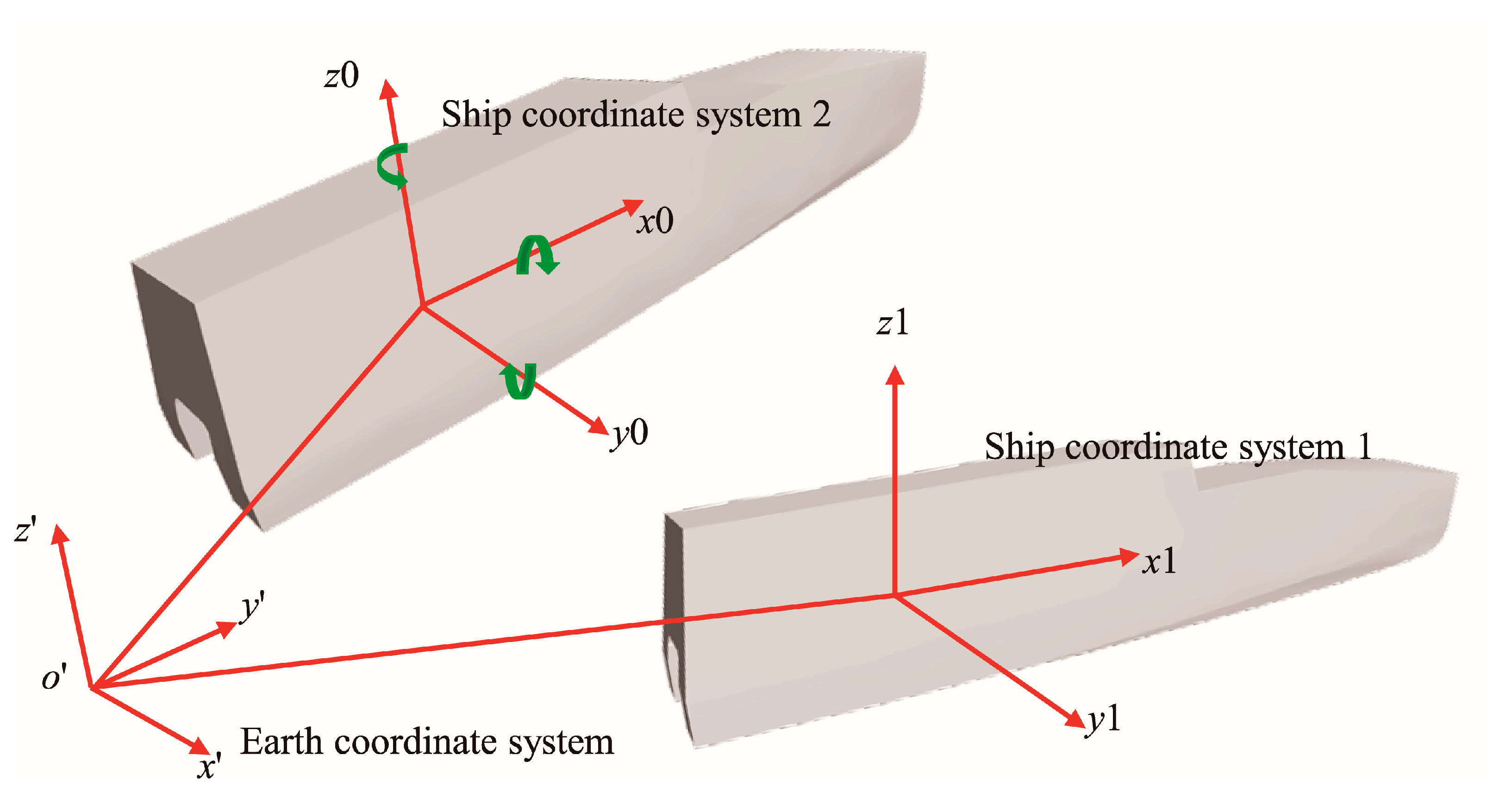
2.3. Degree of Freedom Model

In the simulation, the dynamic fluid body interaction (DFBI) module [18] combined with overset mesh method simulates the heave, pitch, and roll motion of the USV in response to forces exerted by the wave. The 6-DoF (degree of freedom) solver computes fluid forces, moments, and gravitational forces on the USV, and pressure and shear forces were integrated over the surfaces. Two coordinate systems were applied to solve the 6 degrees of freedom equation. One is called the initial coordinate system (earth coordinate system $o^{\prime }{x}^{\prime }{y}^{\prime }{z}^{\prime }$), the other is called the non-initial coordinate system (hull coordinate system $oxyz$), as shown in Figure 2.

The forward direction of the USV is the positive direction of the x-axis, the positive direction of the y-axis points to the port side of the ship, and the z-axis points to the sky. According to the right-hand rule, in the heave motion of the ship, the positive value is the forward motion to the z-axis, and the negative value is the motion to the bottom. In the rolling motion of the ship, the positive value is about the starboard side of the USV in x-axis, and the negative value is about the port side of the ship in x-axis. In the pitch motion of the ship, the positive value turns around the y-axis with bow diving. The negative value is rotation around the y-axis with bow rising.

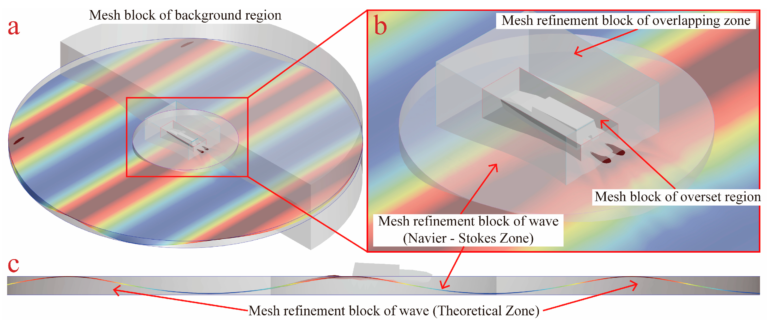
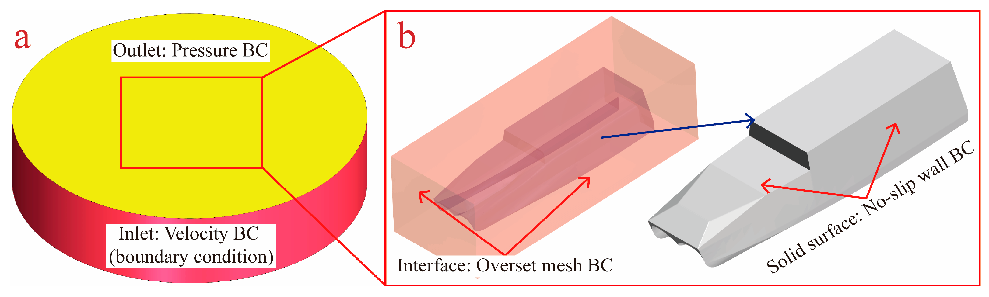
2.4. Computational Domain and Boundary Conditions

The computational domain of the USV in waves is shown in Figure 3. In order to realize the numerical simulation of the USV in different wave directions without changing the calculation grid and other conditions, the cylindrical calculation area is used.

In order to ensure the full development of numerical wave and wake, there were enough interaction and fluid development areas between the USV and free surface in the domain. The axial range of the calculation area is −5.5 L_oa ≤ x ≤ 5.5 L_oa, the spanwise range is −5.5 L_oa ≤ x ≤ 5.5 L_oa, and the vertical range is −1.25 L_oa ≤ z ≤ 2.1 _Loa, where L_oa is the total length of the USV. The boundary conditions are shown in

Table 2. Boundary conditions.

Boundary Name	Boundary Conditions
Inlet	1. Velocity inlet; 2. Fifth order Stokes waves based on VOF components of water vapor; 3. The relative velocity of the USV is 18 kn; 4. The turbulence intensity is 0.01.
Outlet	1. Pressure outlet; 2. Fifth order Stokes waves based on VOF components of water vapor; 3. Fifth order Stokes wave hydrodynamic pressure.
Bottom	Same as the inlet boundary condition
USV hull	No-slip wall
Boundary of Overset region	Overset mesh interface

.

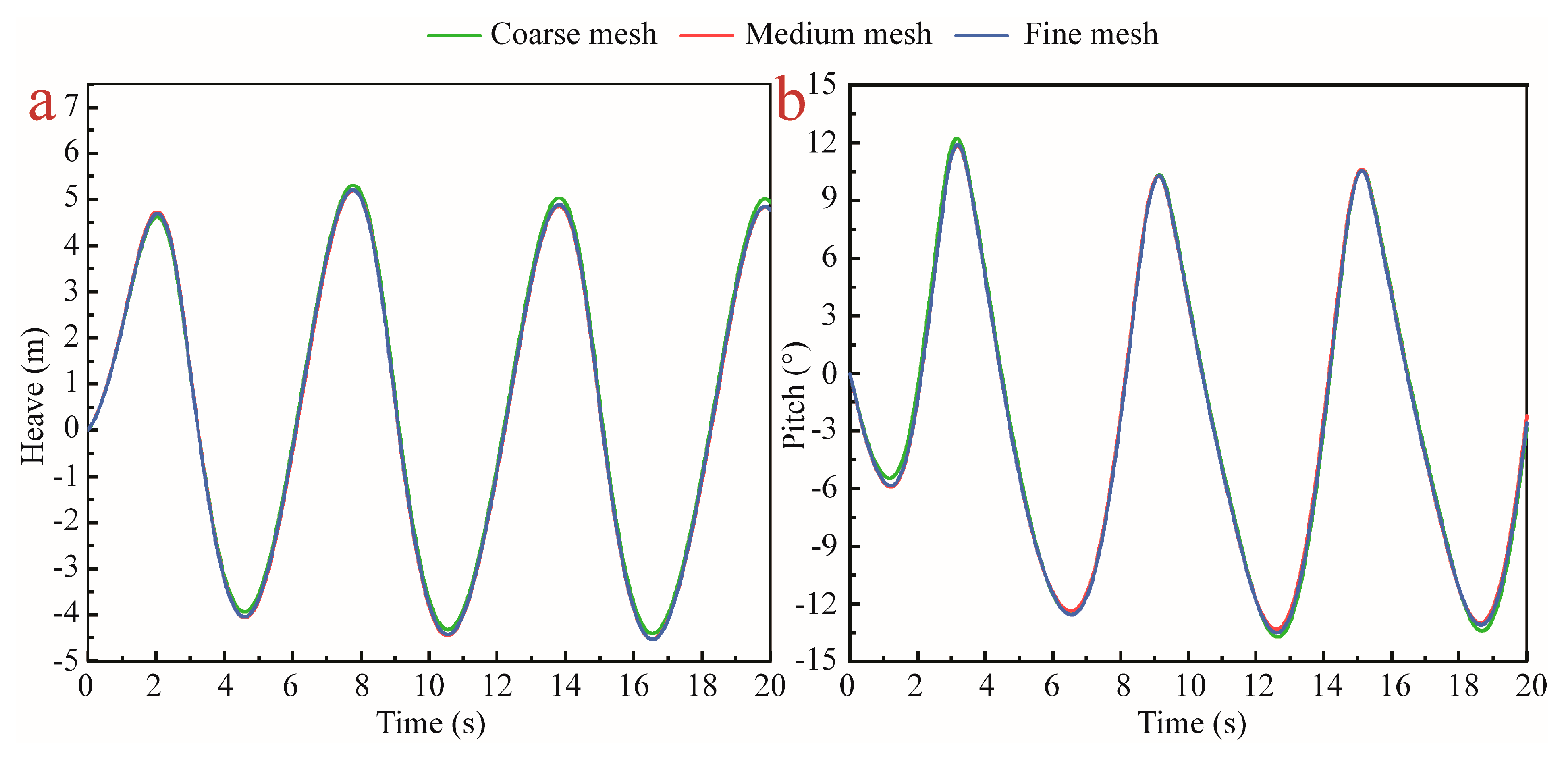
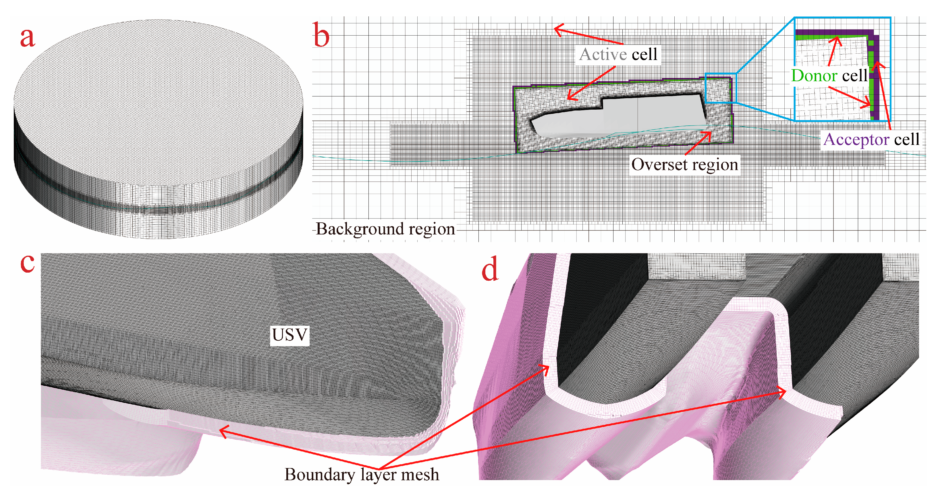
2.5. Computational Mesh and Sensitivity Study

The mesh refinement blocks of the computational domain are shown in Figure 4, and Figure 4a is the mesh block of the background region, Figure 4b is the mesh refinement blocks of the overlapping zone and overset region, and Figure 4c is the mesh refinement blocks in the free surface wave zone. There are two mesh refinement blocks in the free surface wave zone, namely mesh refinement block of wave (Navier–Stokes Zone) and mesh refinement block of wave (Theoretical Zone), a mesh refinement block for the overlapping zone, a mesh refinement block for the overset region. For the wave zone, the Aspect Ratio (AR = length of the cell/height of the cell) of the mesh refinement in the free surface wave was 2. Moreover, about 40 cells per wave height (wave height = 9.0 m) and 300 cells per wavelength (wavelength = 150 m) according to the Aspect ratio. The mesh size of the overset boundary in the overset region was the same as the mesh size of the overlapping zone, thus as to facilitate data transmission between background region and overset region.

The trimmed meshes and prismatic cell layers around the hull were generated using STAR-CCM+, and three sets of coarse, medium, and fine meshes of varying resolutions were generated and used for mesh sensitivity study. The level of the mesh resolution was changed by adjusting the base size of the meshes while keeping the other settings unchanged, and the total number of coarse, medium, and fine meshes meshes was 7.620, 12.207 m, and 22.220 million, respectively. In the present study, the Cartesian cut-cell method was used to generate the computational mesh. Roy et al. [19] presented methods for assessing the uniformity of the mesh refinement with Cartesian grid, and the mesh refinement ratio $r_G$ was considered as follows:

$$r_G={\left(\frac{N_{fine}}{N_{coarse}}\right)}^{1/d}$$

(3)

where the total number of meshes is noted as N, d is the dimensionality of the computing problem, and its value in the present study is 3. The mesh refinement factor for the fine/medium and medium/coarse meshes was 1.22 and 1.17, respectively. The mesh refinement ratio of fine to medium (medium to coarse) grids was approximately 1.2, which was consistent with references [20]. The heave and pitch motion plots of USV at 7 level sea state with different meshes are shown in Figure 5. The comparative analysis indicates that the three meshes with different resolutions were all able to accurately predict and calculate the motion of the USV in a high sea state. Compared to the fine grid, the use of a medium grid can reduce the computational cost considerably and still achieve a tolerable level of numerical accuracy. Thus, the meshes generation for the cases of this paper was dependent on the arrangement of a medium mesh. The time step in all cases was 0.005 s, and the free surface convection courant number meets the requirement, that is, Courant–Friedrichs–Lewy (CFL) number (CFL = U △t/△x, where CFL is the courant number, U is the reference velocity, △t is the time step, and △x is the grid size) needs to be less than 1.

The medium computational mesh of the USV in waves is shown in Figure 6, and Figure 6a is the overall meshes of the computational domain, Figure 6b is the overset mesh, and local mesh refinement of the free surface, overlap area, Figure 6c,d are the meshes around the hull and boundary layer mesh.

3. Numerical Wave Tank and Verification

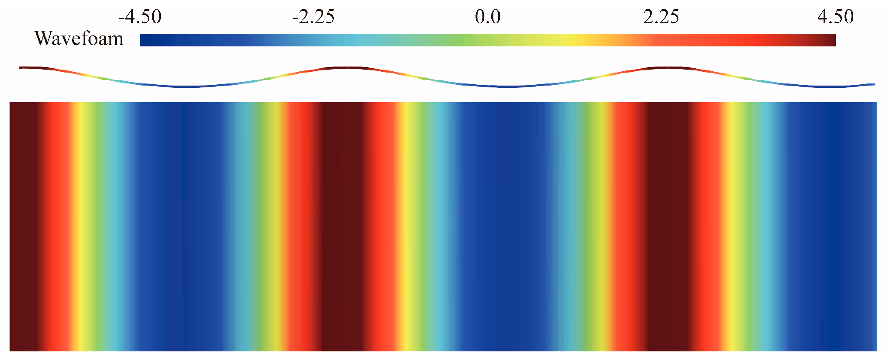
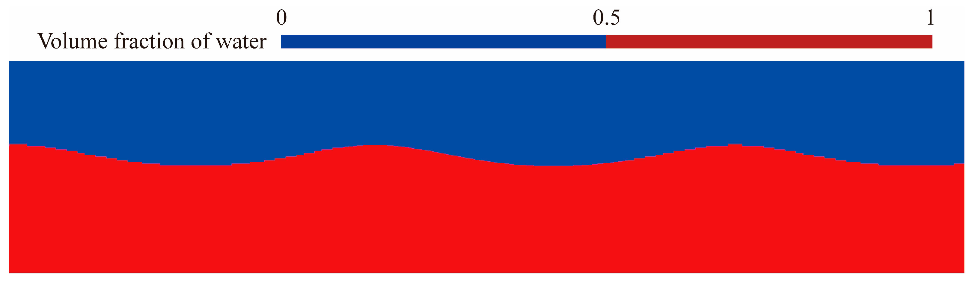
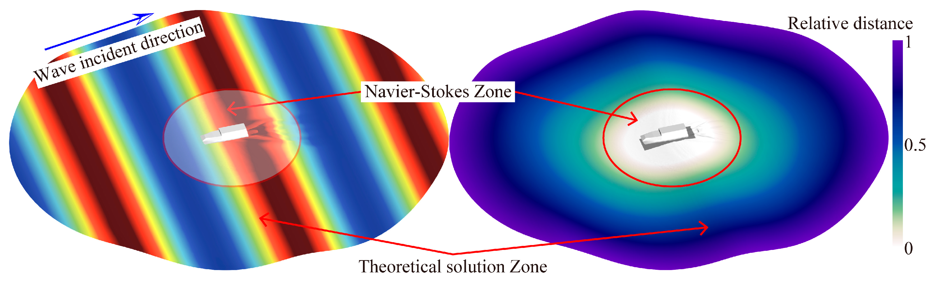
3.1. Numerical Wave Tank

Wave generation of numerical wave tank was realized via the inlet and outlet boundaries, referred to as the boundary velocity input method. The velocity and pressure profile over the water depth of waves were set at the inlet and outlet boundaries. The wave generated by the fifth-order was more similar to a real wave than that generated by the first-order method, and a fifth-order wave modeled by approximating the fifth-order to the Stokes theory of waves was used as the numerical wave type in the study. The detailed description of wave profile, including the wave phase velocity, depends on the water depth, wave height, and current of fifth-order VOF waves can be found in the studies conducted by Fenton [21].

When numerical wave propagates to the physical boundary, the boundary wave reflection usually occurs, and the boundary wave reflection will interfere with the calculation and wave quality. The Euler-overlay method (EOM) [22] was adopted to address the reflections of surface waves at boundaries. Detailed numerical wave tank and illustration of the Euler overlay method are shown in Figure 7. There are three zones, namely the inner CFD (Navier-Stokes zone), overlay, and outer Euler wave (theoretical solution zone) zones. The overlay zone located between the outer Euler and inner CFD zones gradually blends the CFD and Euler solutions, applying source terms to VOF and momentum equations. The reflections of surface waves are addressed via the forcing solution of the discretized Navier–Stokes equations towards theoretical solution over a specified distance, which increases the calculation efficiency and reduces the calculation time cost owing to its use of reduced-size mesh refinement in the solution domain theoretical solution zone. A detailed explanation and application of the Euler-overlay method (EOM) can be seen in the references [23,24,25,26].

The incident direction of waves and the sailing direction of the USV is shown in Figure 8.

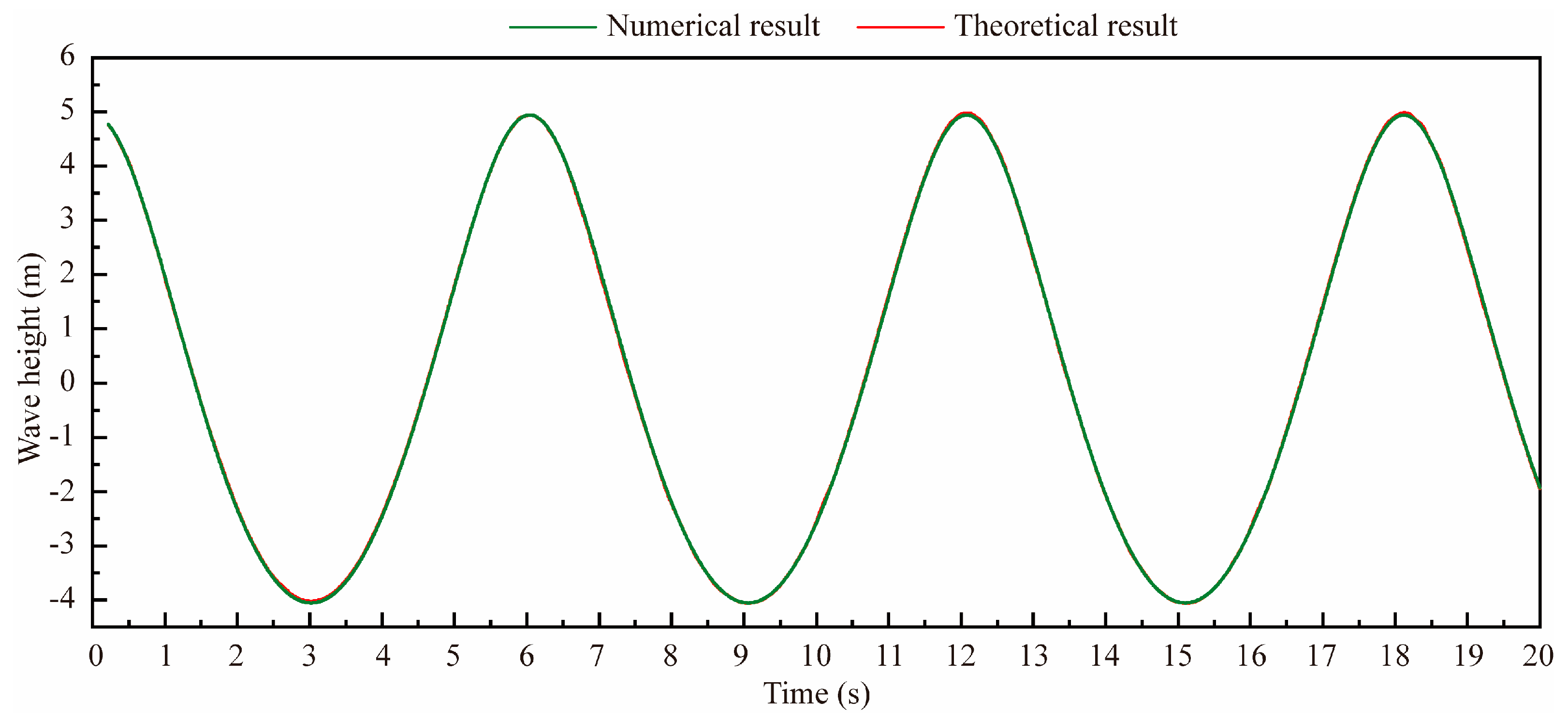
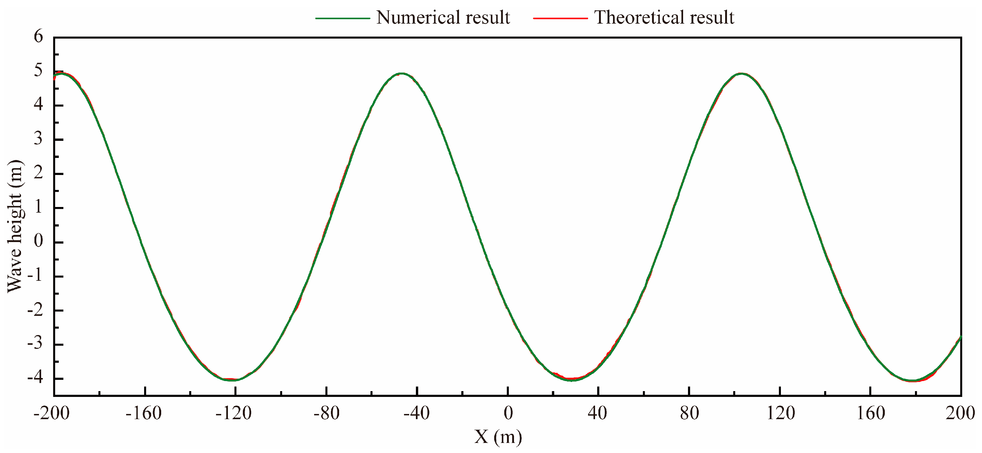
3.2. Numerical Wave Tank Verification

In the verification study of the numerical wave, the fifth-order Stokes waves with level 7 sea state were simulated, and the obtained results were compared with the theoretical solutions (See Section 3.1) to verify the accuracy of the numerical wave tank. To record the change in water surface, a wave height detection point was set at the center of the tank. The wave height versus time is shown in Figure 9. The wave height position point distribution along the propagation direction is shown in Figure 10. The red curve is the numerical simulation result, and the green circle is the theoretical analytical solution. It can be seen from Figure 9 and Figure 10 that the numerical simulation wave is in good agreement with the theoretical analytical solution of the wave.

The waveform of numerical wave propagation after 20 s is shown in Figure 11. The distribution of water and air composition after 20 s of numerical wave propagation is shown in Figure 12. The waveform and the distribution of water and air components are well preserved after propagation for 20 s in Figure 11 and Figure 12. The verification of numerical results and theoretical analytical solutions can ensure that the calculation grid and calculation strategy of this study meet accuracy requirements, and the numerical wave tank is reliable.

4. Results

In this paper, the motion of the USV in waves under 5 level and 7 level states is studied. The waves in the real sea state were all irregular waves. In this study, the waves in 5 level and 7 level sea states were simplified and analyzed by regular waves. The wavelength, height, and period of the simplified regular wave under 7 level states were 150 m, 9.0 m, and 9.629 s, respectively. The wavelength, height, and period of the simplified regular wave under 5 level states were 100 m, 3.25 m, and 7.961 s, respectively.

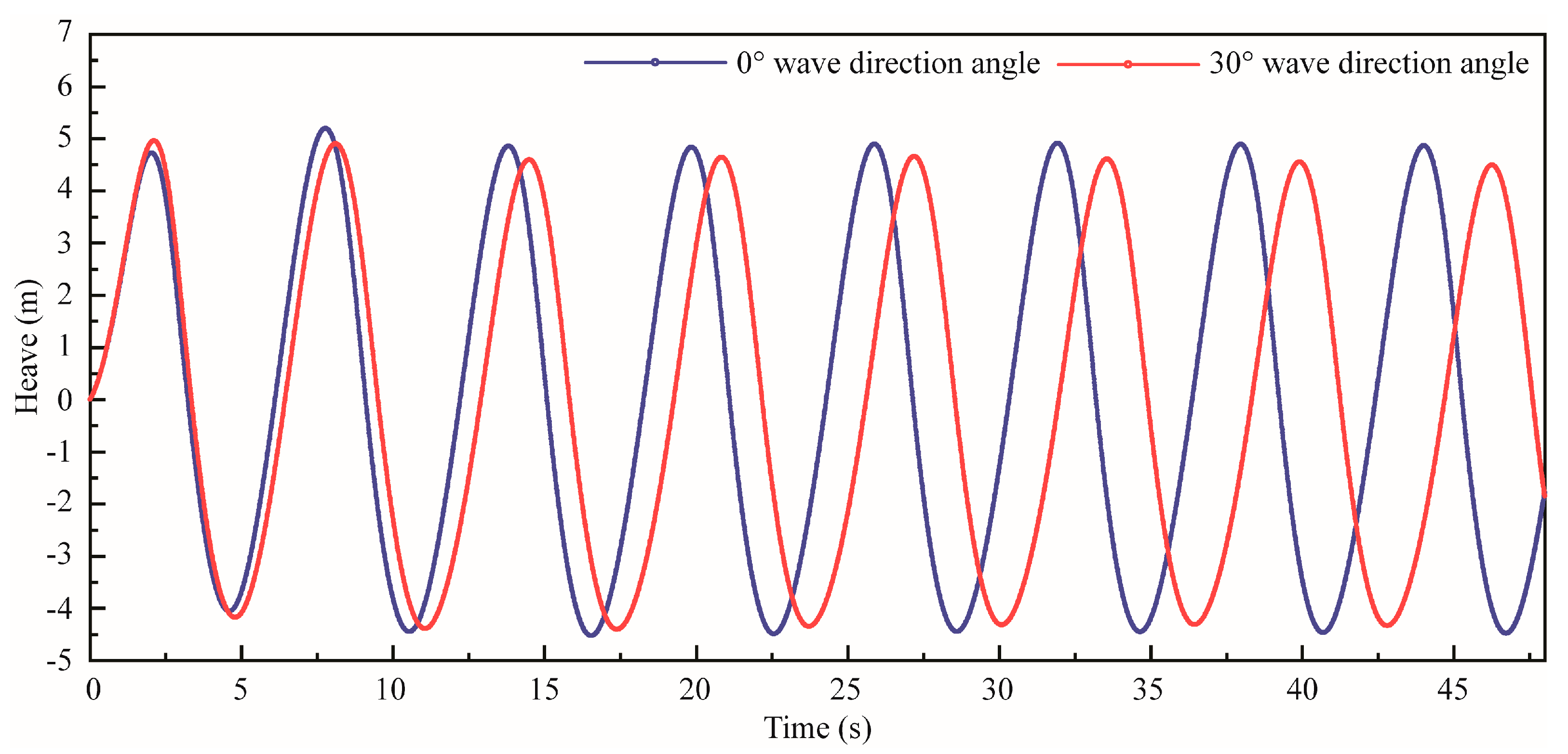
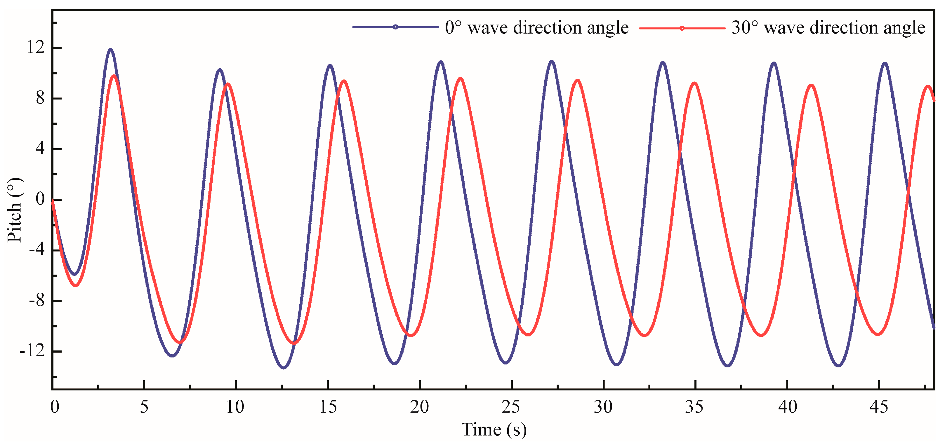
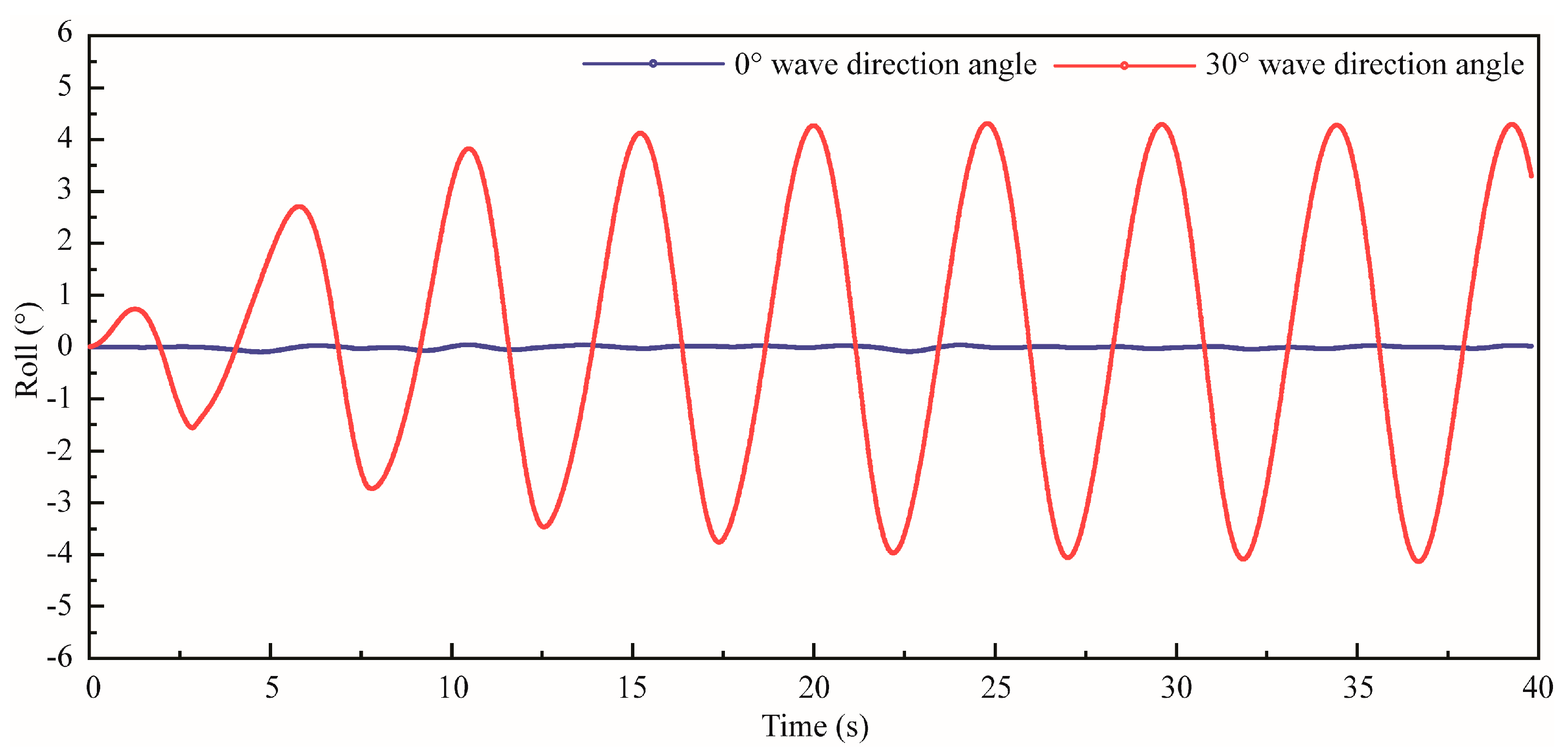
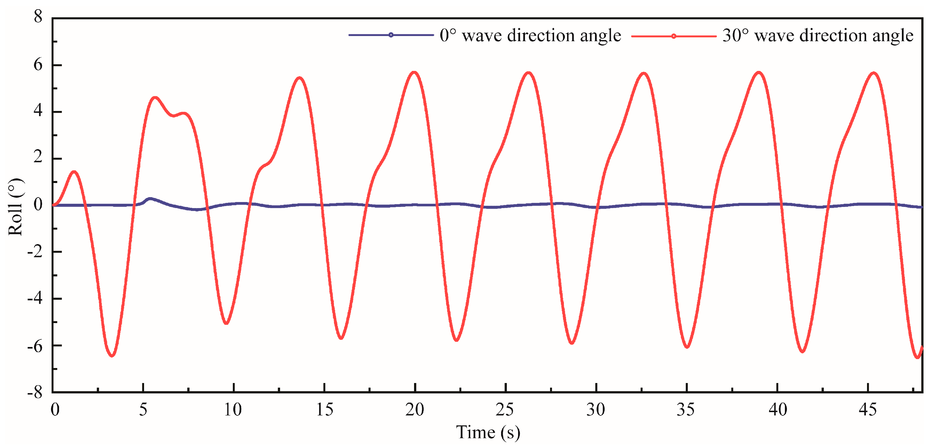
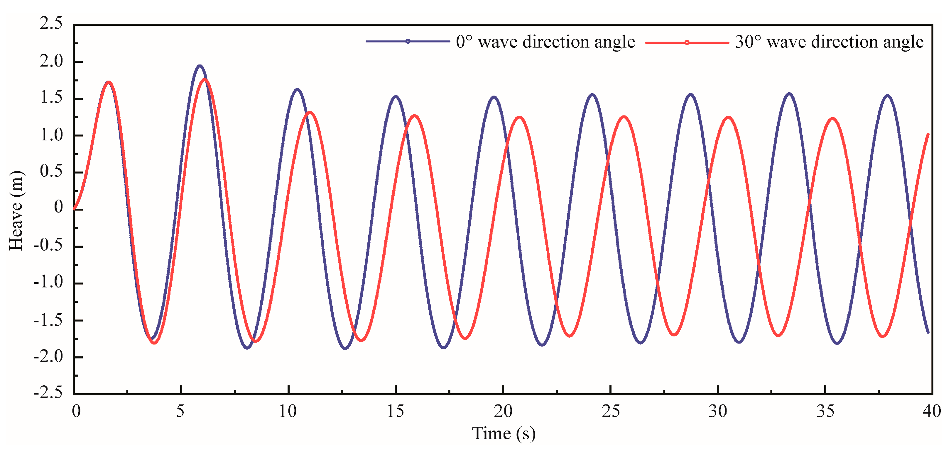
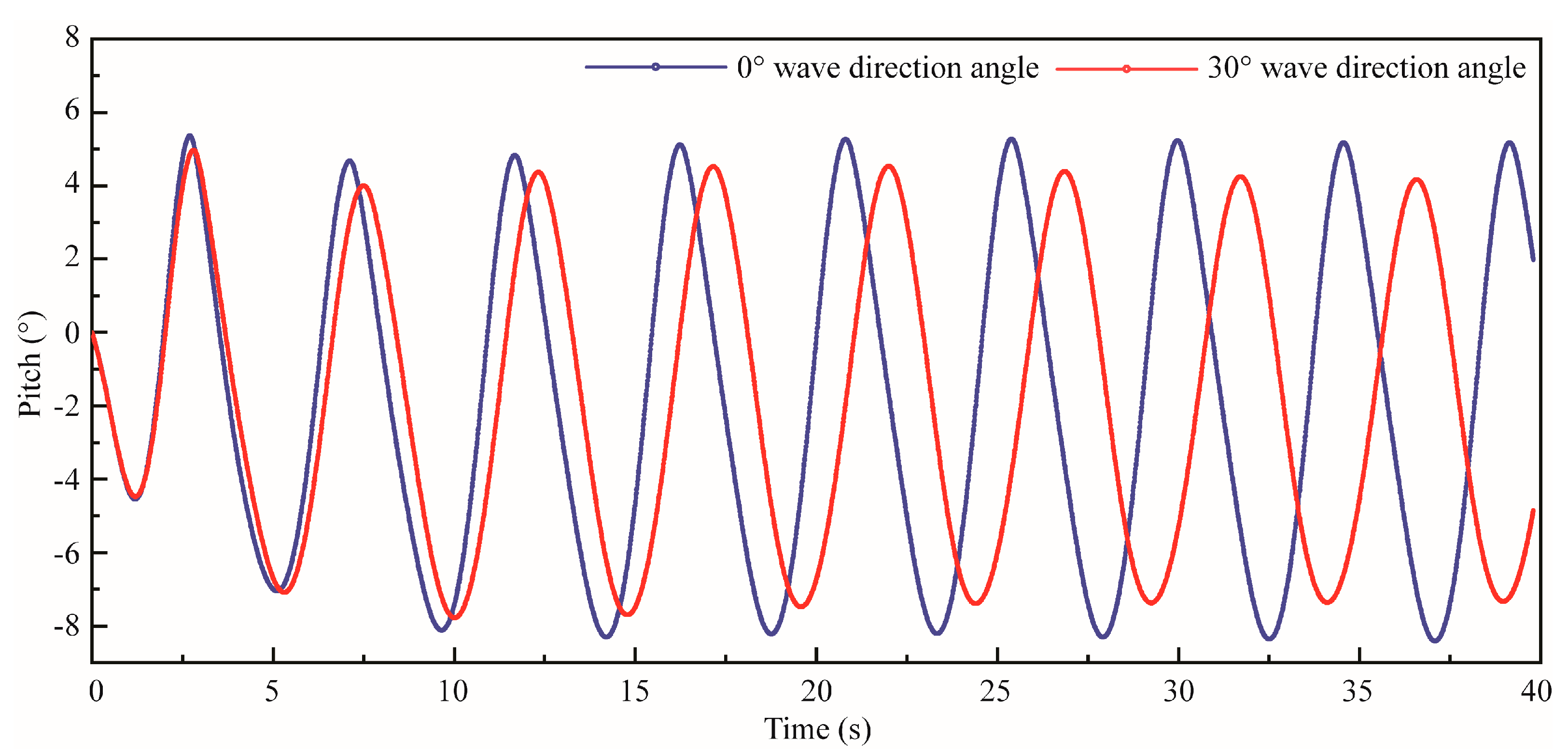
4.1. Six Degrees of Freedom Motion with Time History

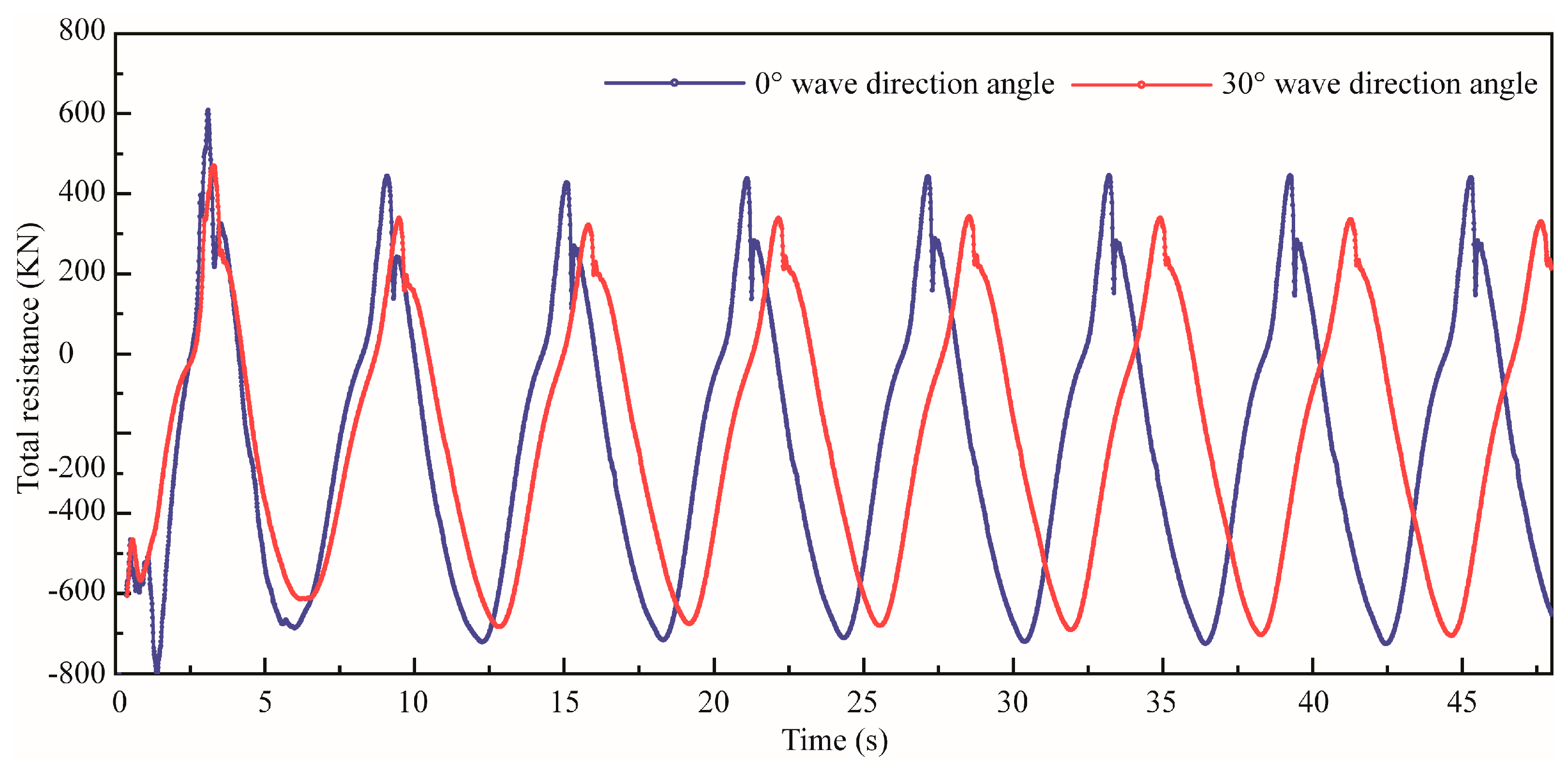
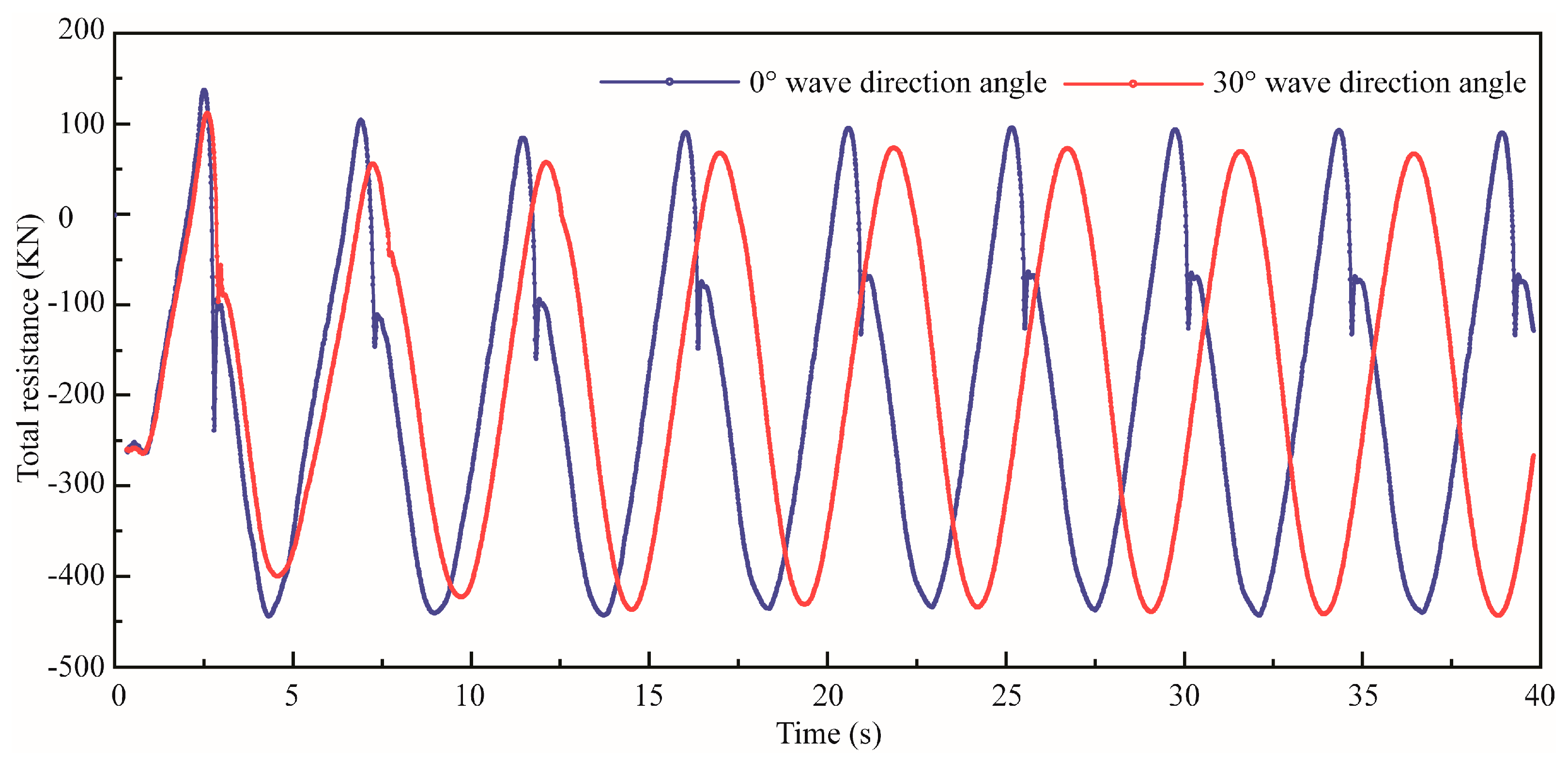
The six degrees of freedom motion process was simulated at the 0° and 30° wave direction angles under 7 level sea state. Figure 13, Figure 14 and Figure 15 show the heave motion, pitch motion, and roll motion with different wave direction angles, respectively, at 7 level sea state. At the 0° and 30° wave direction, the heave amplitude ranged from −5 m to 5 m, showing periodic variation. The pitch angle ranged from −12 to 12 degrees at 0° wave direction and from −12 to 10 degrees at 30° wave direction. The positive value for bow raising and the negative value for bow diving. The results show that the stable roll angle of the USV was very small in the 0° wave direction, which was close to 0 degrees and had no significant periodicity. The roll angle of the USV was obvious in the 30° wave direction, which ranged from −7 to 6 degrees.

Figure 16, Figure 17 and Figure 18 show the heave motion, pitch motion, and roll motion with different wave direction angles, respectively, at 5 level sea state. At the 0° and 30° wave direction, the heave amplitude ranged from −1.75 m to 1.75 m, showing periodic variation. The amplitude of heave in the 0° wave direction was slightly larger than that in the 30° wave direction, and the period of heave change in the 0° wave direction was slightly smaller than that in the 30° wave direction. The pitch angle ranged from −7 to 5 degrees at the 0° and 30° wave direction. The amplitude of pitch in the 0° wave direction was slightly larger than that in the 30° wave direction. The positive value for bow raising and the negative value for bow diving. The results show that the stable roll angle of the USV was very small in the 0° wave direction, which was close to 0 degrees and had no significant periodicity. The roll angle of the USV was obvious in the 30° wave direction, which ranged from −4 to 4 degrees.

In summary, the six degrees of freedom motion of the USV under different sea states basically presents periodic changes, and the motion amplitude of the 0° wave direction was slightly greater than that of the 30° wave direction. The rolling motion was not obvious at 0°, and the motion of the USV under different sea states and does not exceed the stable range of motion, which meets the stability requirements, and there was no overturning phenomenon.

4.2. Resistance

Figure 19 and Figure 20 show the total resistance curves in different wave directions. The total resistance in the 0° wave direction was slightly greater than that in the 30° wave direction.

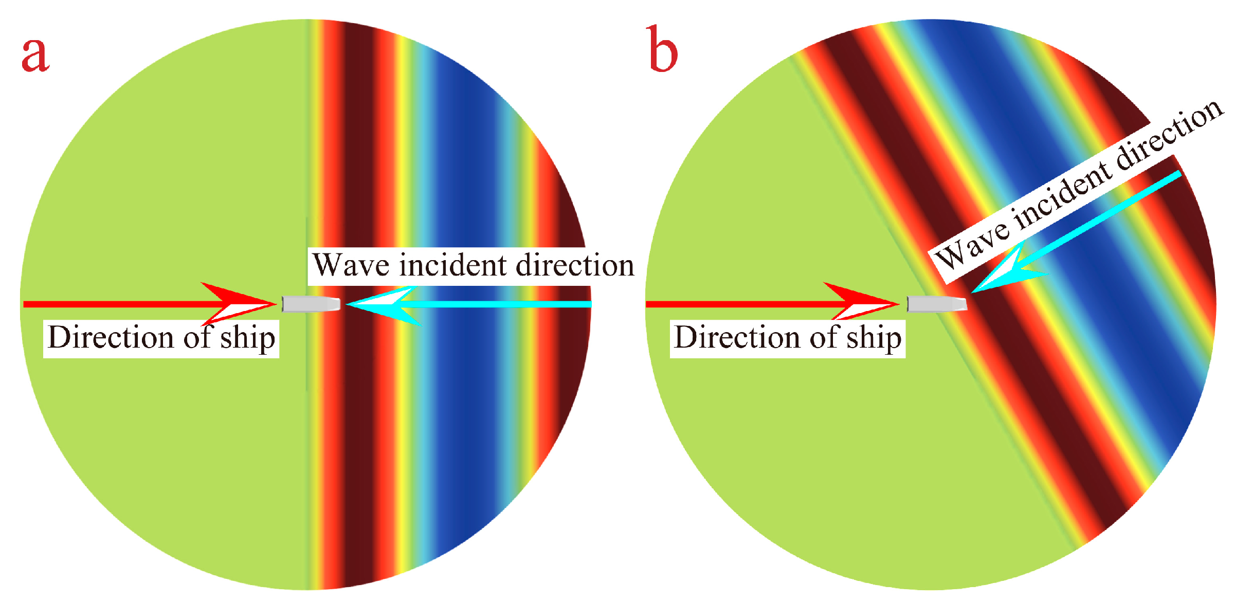
4.3. The Attitude of USV in Waves at Typical Times under 7 Level Sea State

Figure 21 and Figure 22 show the attitude of the USV in waves at a typical time when the wave direction was 0° and 30° under 7 level sea state, respectively. T0 is the period of the wave. When T = 0 to 1/4T0, the incident wave peak propagates from the bow to the stern, and bow diving happens. The heave amplitude first increases and then decreases along the positive direction. When T = 1/4T0 to 2/4T0, the wave trough gradually propagates to the stern, the heave amplitude gradually increases along the negative direction, the pitch amplitude gradually increases in the positive direction, and the bow rising happens. When T = 2/4T0 to 3/4T0, the wave peak is transmitted to the bow, the heave amplitude reaches the maximum in the negative direction, and the pitch amplitude reaches the maximum in the positive direction, resulting in the maximum bow rising. When T = 3/4T0 to 4/4T0, the wave trough is transmitted to the bow position, the heave amplitude reaches the maximum value in the positive direction, and the pitch amplitude reaches the maximum value in the negative direction. The maximum bow diving happens. When T = 4/4T0 to 5/4T0, the wave trough gradually transmitted to the stern, and the bow rising happens. The motion law of the 0° wave direction and 30° wave direction was consistent, and the motion amplitude was slightly different. The motion amplitude of the 0° wave direction was larger than that of the 30° wave direction. In the whole process of USV movement around the waves, the stability of the USV meets the stability requirements, and no capsizing occurs.

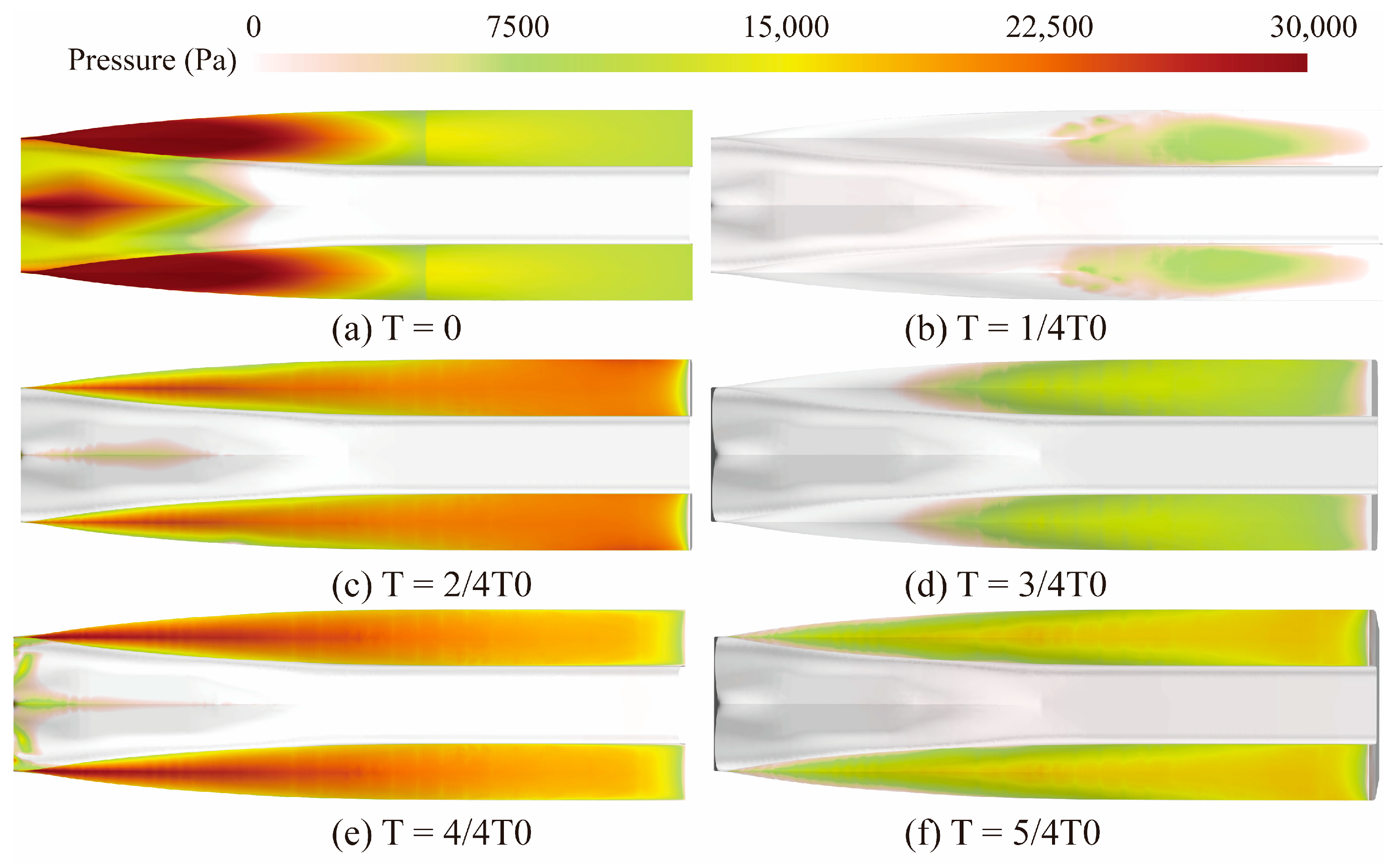
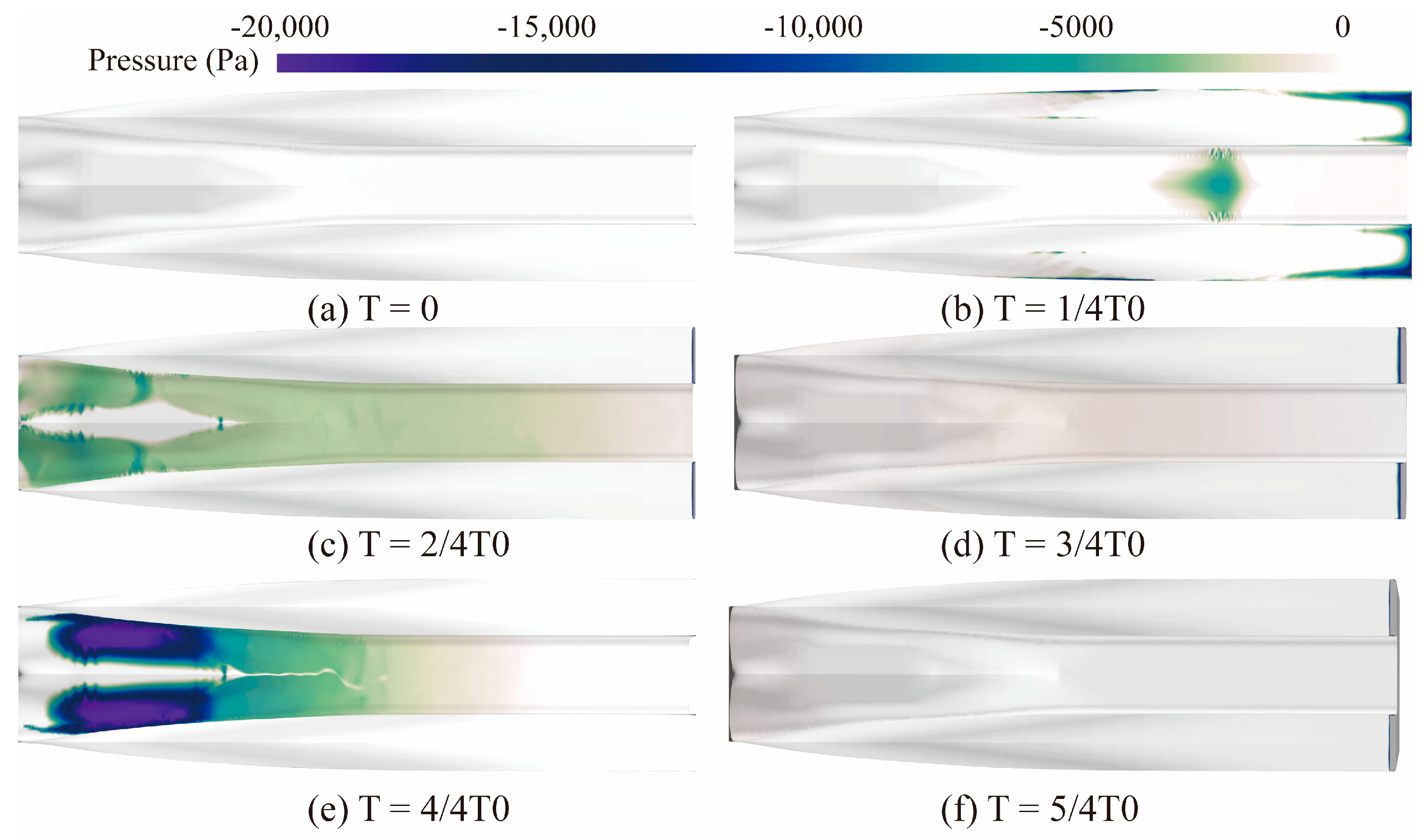
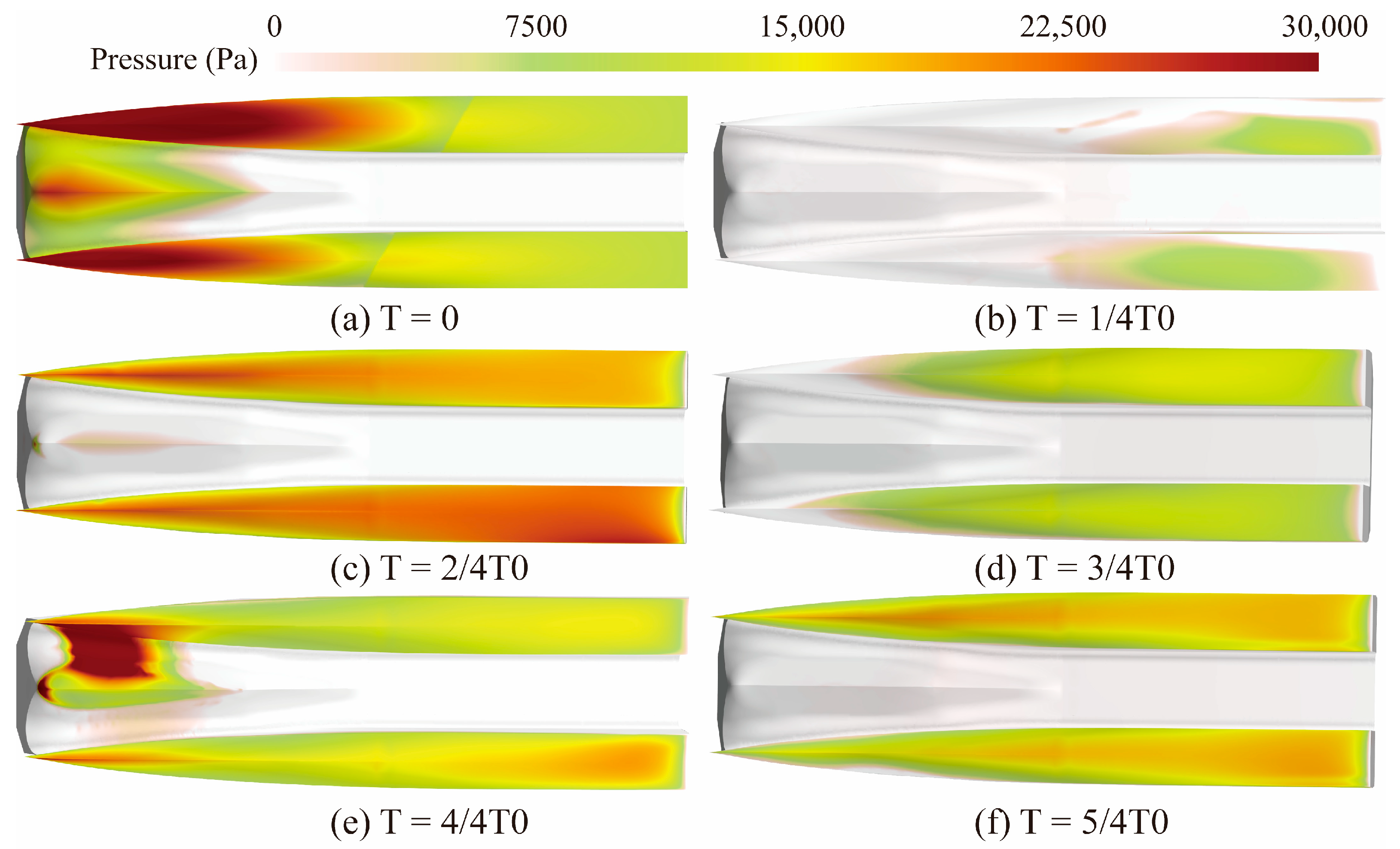
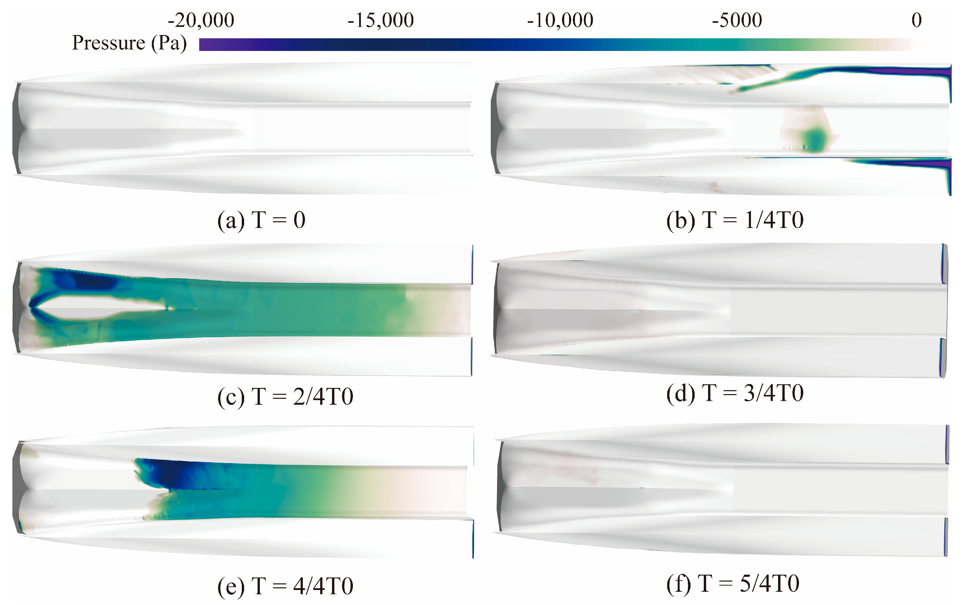
4.4. Pressure Distribution at the Bottom of the USV at Typical Times under 7 Level Sea State

Figure 23 and Figure 24 show pressure distribution at the bottom of the USV when the wave direction was 0° under 7 level sea state, respectively. The positive pressure at the bottom of the USV was mainly concentrated in the two side body areas, and the negative pressure was mainly concentrated in the area between the side bodies. In addition, when T = 0, the USV was in the initial wave state and had a large static pressure. The maximum pressure reached 29,570 Pa. When T = 2/4T0 and T = 4/4T0, the bottom pressure was large, including a large positive pressure and negative pressure, and the area was the largest. When T = 4/4T0, the negative pressure reached the maximum value −18,738 Pa.

Figure 25 and Figure 26 show pressure distribution at the bottom of the USV when the wave direction is 30° under 7 level sea state, respectively. When T = 0 and 4/4T0, the USV has a large static pressure. The maximum pressure reached 28,390 Pa. When T = 2/4T0 and T = 5/4T0, the bottom positive pressure was relatively large. When T = 2/4T0 and 4/4T0, the bottom negative pressure was large. The maximum negative pressure reached −19,520 Pa.

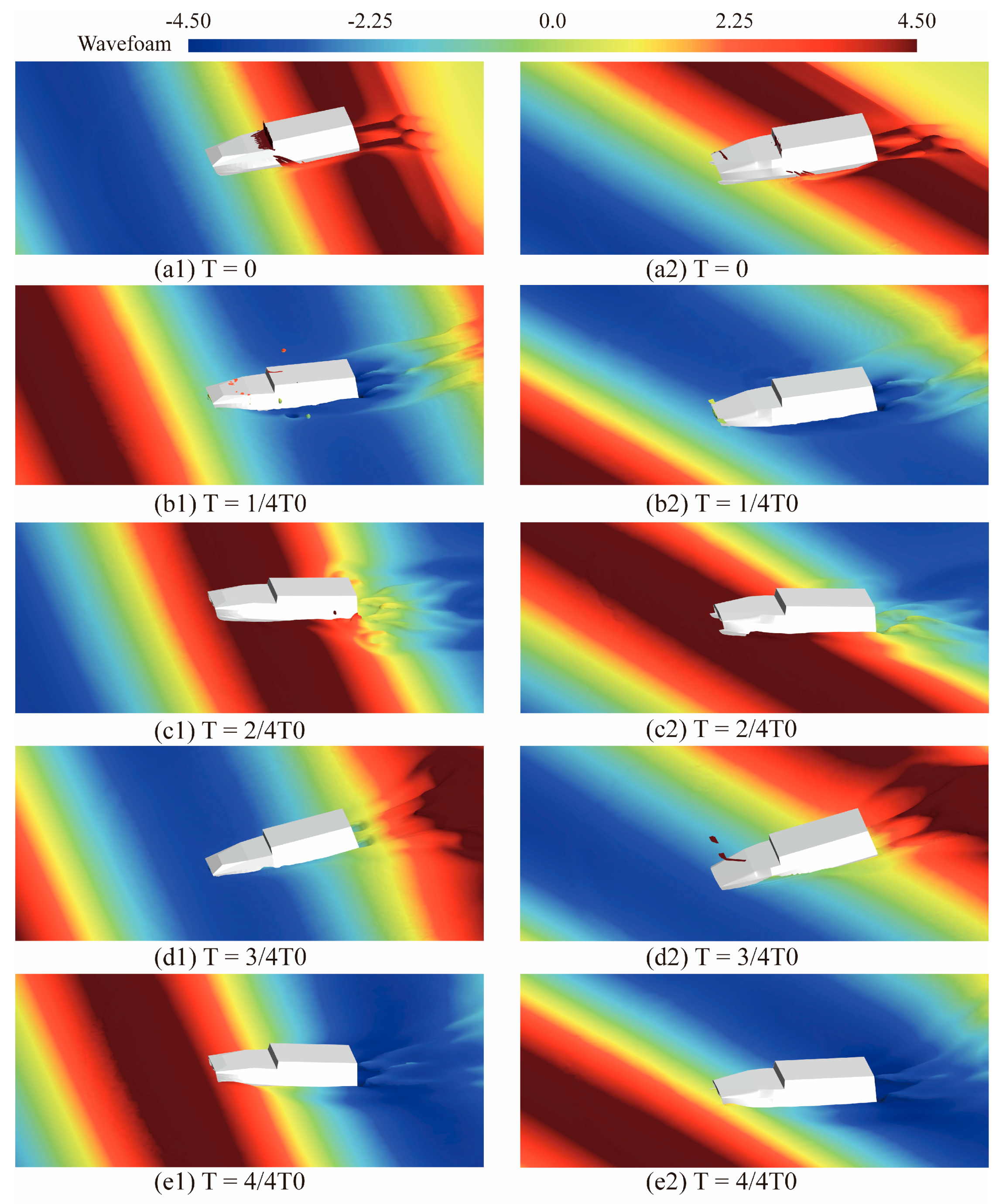
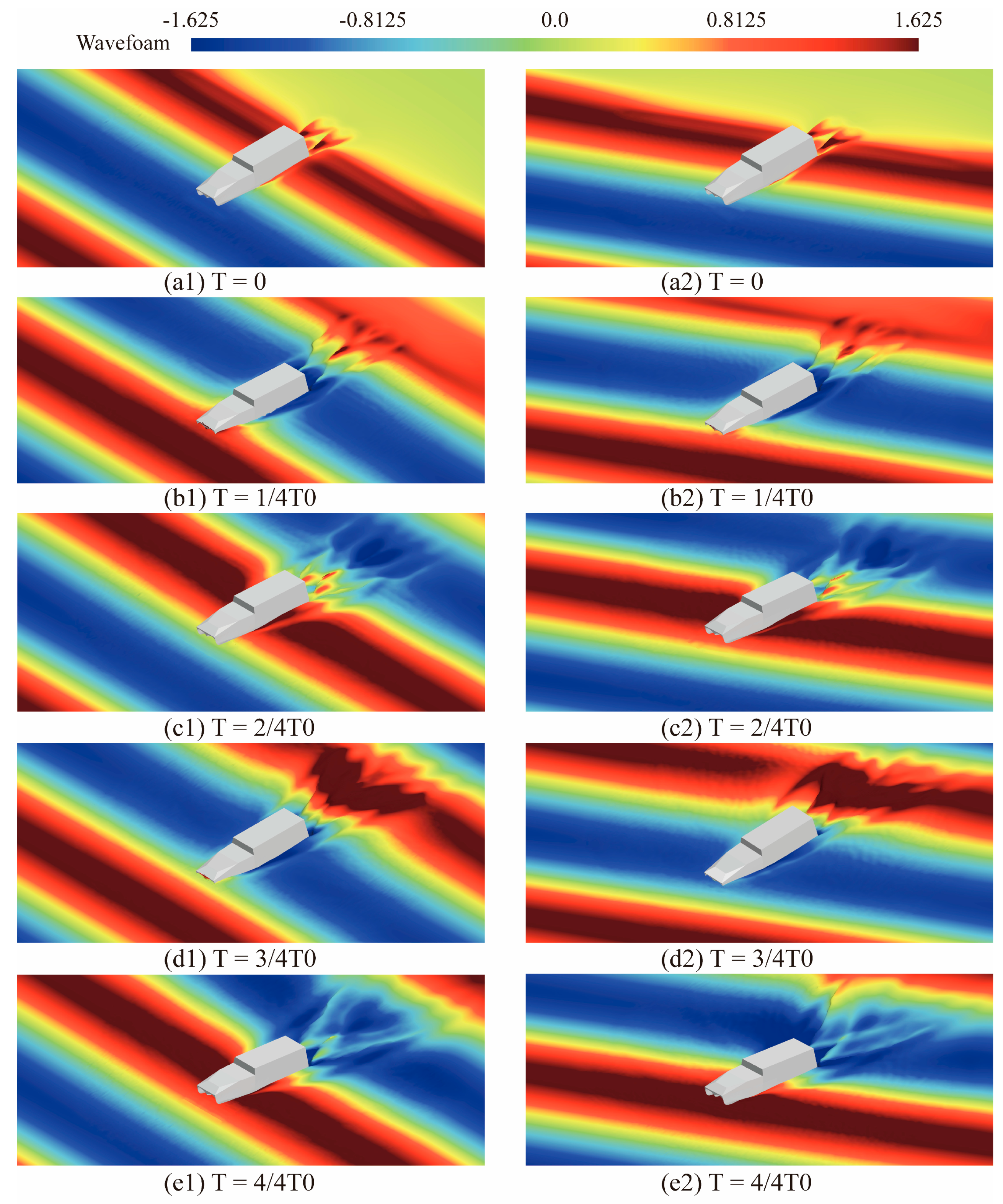
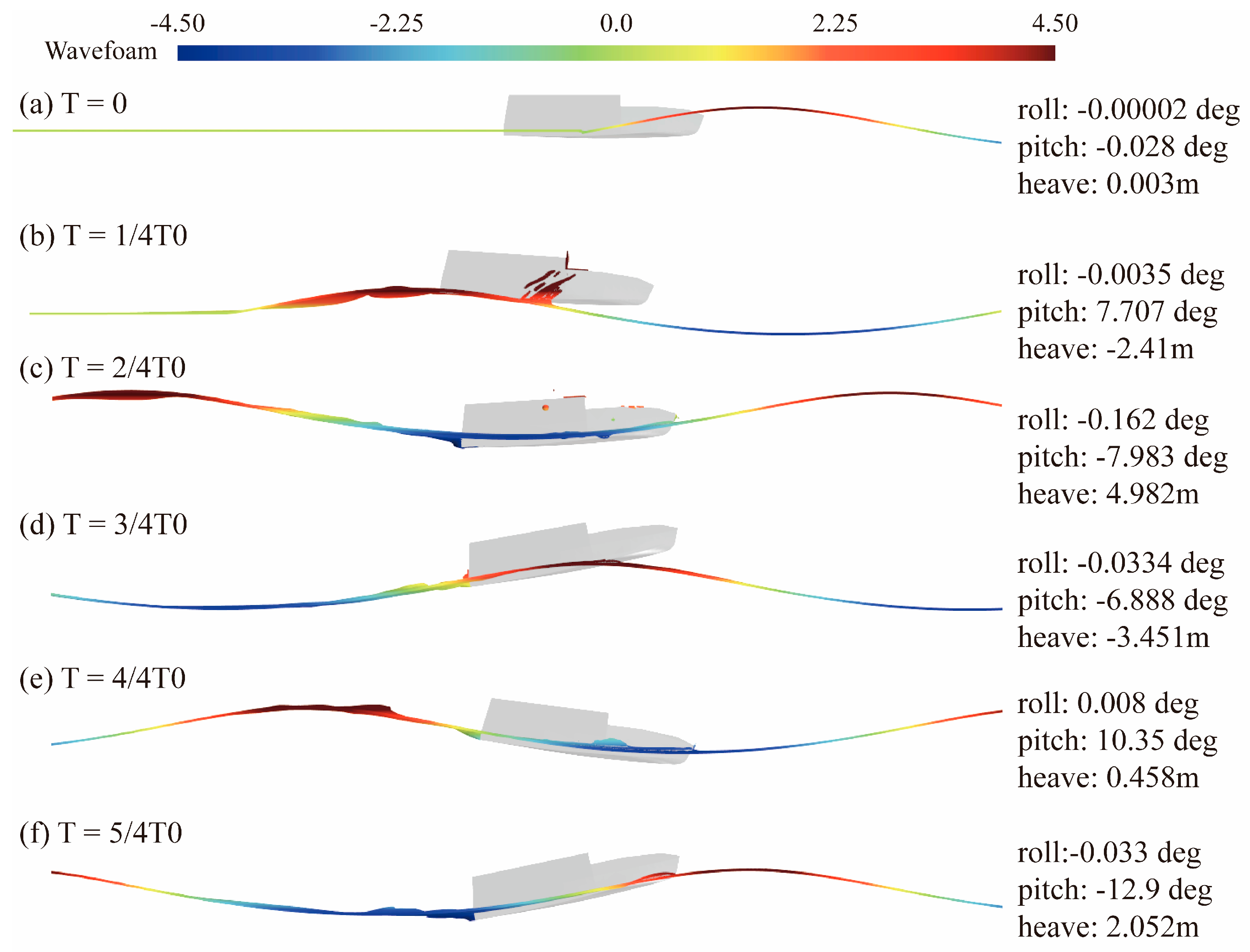
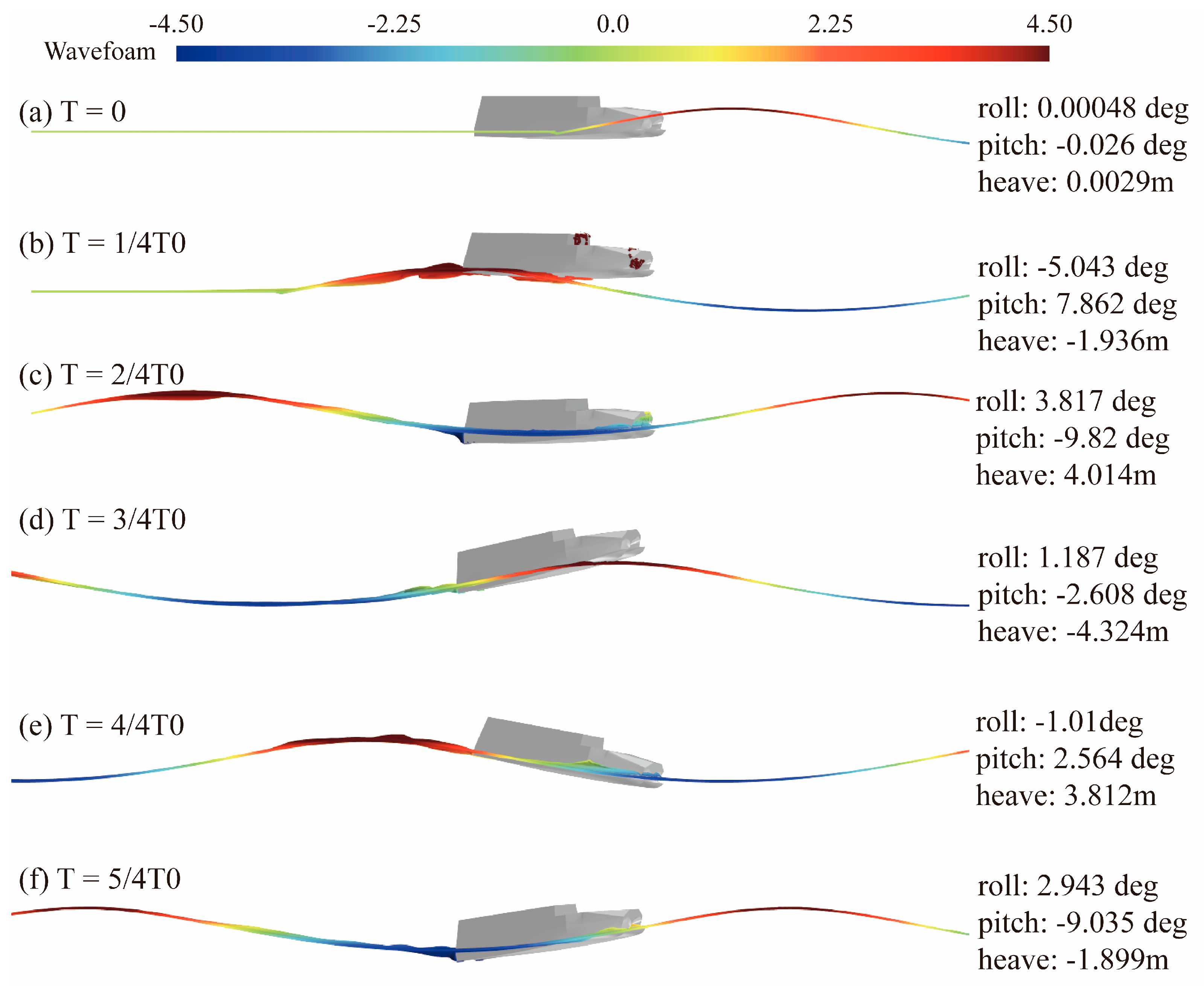
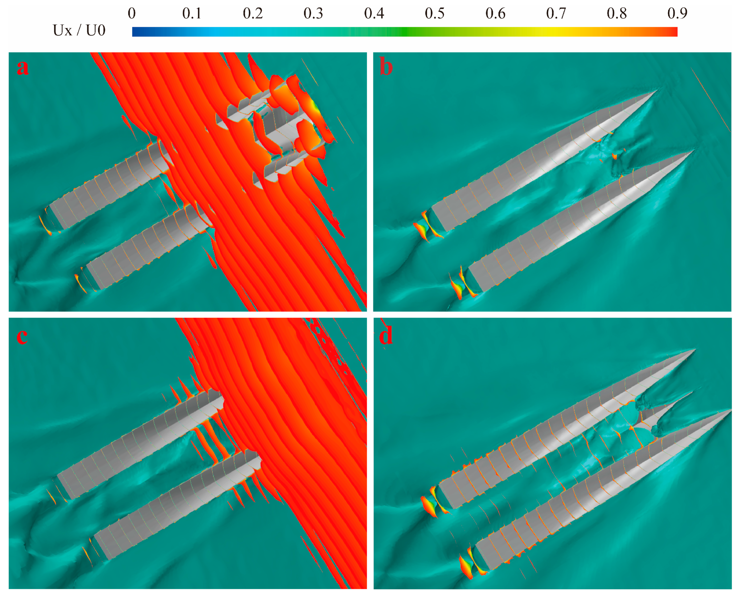
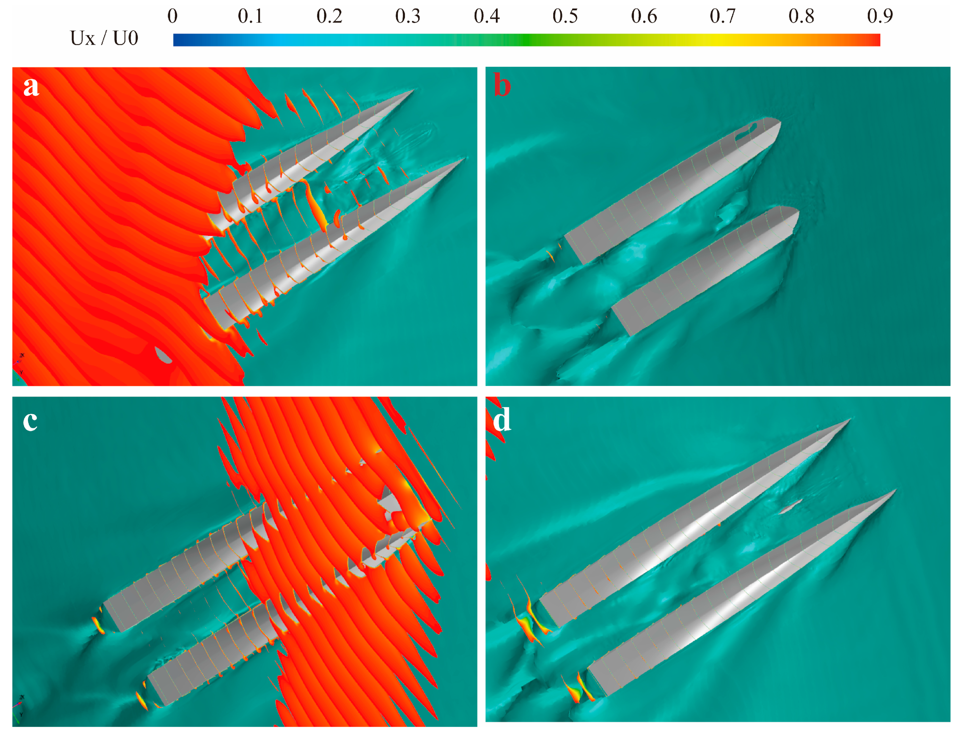
4.5. Free Surface Waveform and USV Three-Dimensional Attitude

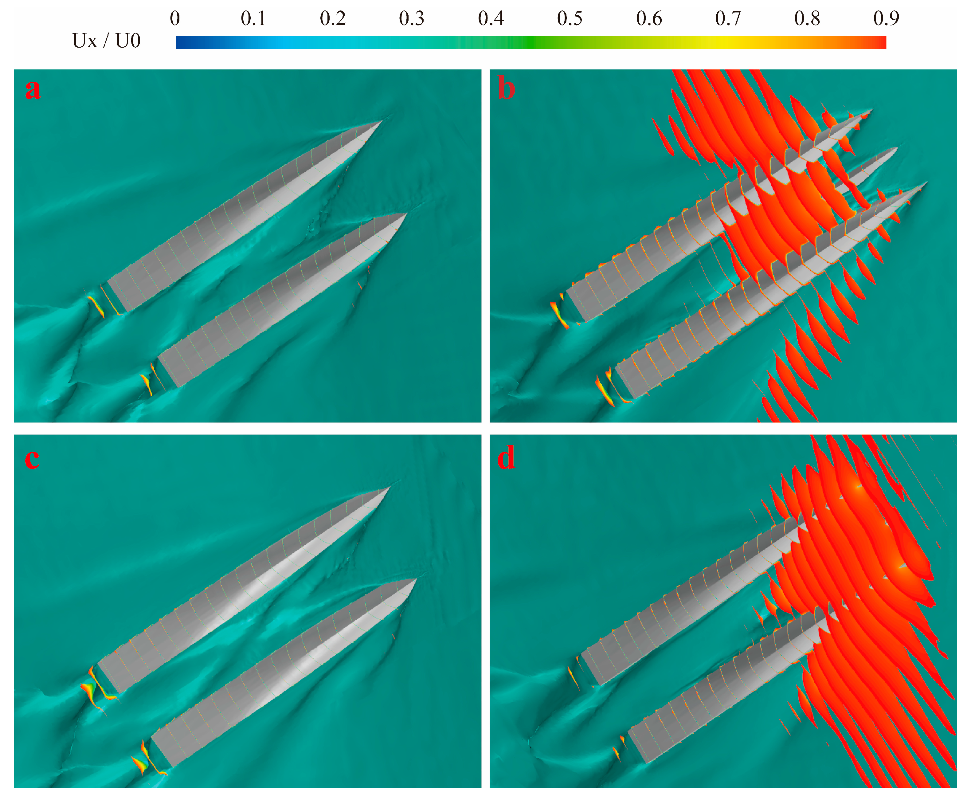
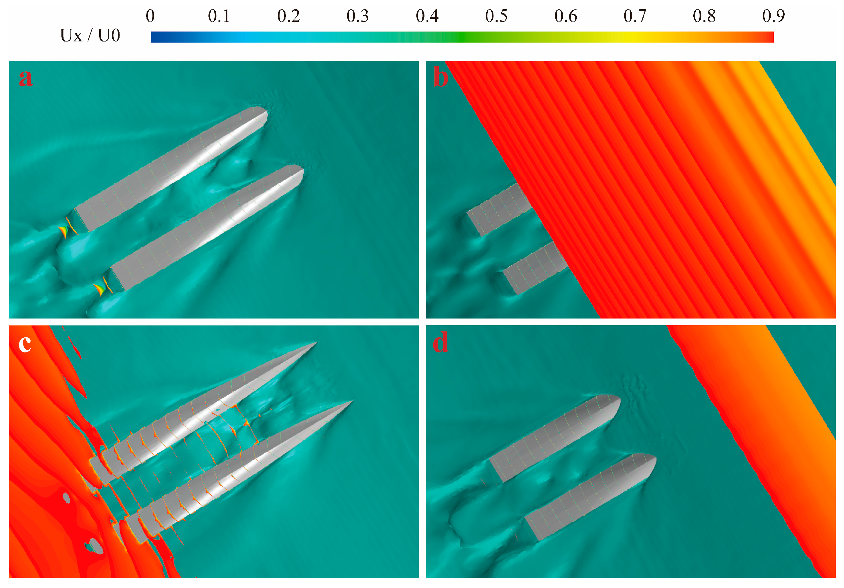
Figure 27 and Figure 28 show free surface waveform and USV three-dimensional attitude at different times in different wave directions under 5 level and 7 level sea states, respectively. It can be seen from Figure 27 that when the wave direction was 0° and T = 0 to 1/4T0, the bow was in the wave trough, and the stern passes through the wave peak position. The bow diving happens slightly. At this time, the stern causes wave and wake. When T = 1/4T0 to 2/4T0, the whole USV hull is in the wave trough section, and the USV has large sinking and bow diving. When T = 2/4T0 to 3/4T0, the whole USV is in the wave peak section, and the USV begins to rise, which changes from the trim by bow state to the trim by stern state, resulting in bow rising. When T = 3/4T0 to 4/4T0, the ship moves from the wave peak to the wave trough. At T = 4/4T0, the bow is in the wave trough, and the USV sinks and bow diving happens. When T = 4/4T0 to 5/4T0, the USV is between the wave trough and the wave peak and has experienced a change process from bow diving to bow rising. At T = 5/4T0, the stern is in the wave trough, and the bow is in the wave peak. In Figure 28, the process of the USV motion in 30° wave direction is similar, but the bow rising and bow diving amplitude in 30° wave direction are less than the 0° wave direction, and the wave making and wake intensity in stern area are less than the 0° wave direction. The USV rolling is obvious in 30° wave direction. The motion process of the USV at different times under the 7 level sea state follows the wave periodic variation, which is similar to the 5 level sea state. The difference is that the heave and pitch amplitude of the USV under the 7 level sea state is very severe, which is much larger than the 5 level sea state, but it still meets the stability requirements without capsizing.

4.6. Boundary Layer

Figure 29 is the boundary layer represented by slices colored with dimensionless axial velocity limited to U_x/U₀ = 0.9 at 5 level sea state with the 0° wave direction. Among them, Figure 29a–d are the underwater perspectives of T = 1/4T0, T = 2/4T0, T = 3/4T0, and T = 4/4T0, respectively. It can be found that the motion of wave and the USV has a different influence on the boundary layer at different times. When T = 1/4T0, the USV moves from wave trough to wave peak, and the bow just reaches the wave peak position. Most of the bow submerges into the water, and the midship to the bow area has a thick boundary layer. When T = 2/4T0, the whole USV is at the wave peak position (see Figure 22), and the boundary layer is the thinnest. When T = 3/4T0, the whole USV is at the wave trough position (see Figure 22), and the bow is heading to the wave peak with a thick boundary layer at the bow area. When T = 4/4T0, the whole USV is at the wave peak position, the midship and the bow area have the thinnest boundary layer, and the stern area is relatively thick. Figure 30 is the boundary layer represented by slices colored with dimensionless axial velocity limited to U_x/U₀ = 0.9 at 5 level sea state with 30° wave direction. Among them, Figure 30a–d are the underwater perspectives of T = 1/4T0, T = 2/4T0, T = 3/4T0, and T = 4/4T0, respectively. It can be found that the thickness distribution of the boundary layer is very different with the 30° wave direction from that of the 0° wave direction. When T = 1/4T0 and T = 3/4T0, the USV is at the wave trough position, and the boundary layer is thin. When T = 2/4T0, the midship and the bow area are at the wave peak position with a thick boundary layer, and the stern area is relatively thin. When T = 4/4T0, the bow is heading from the wave trough to the wave peak. The bow area has a thick boundary layer.

Figure 31 shows the boundary layer represented by slices colored with dimensionless axial velocity limited to U_x/U₀ = 0.9 at 7 level sea state with the 0° wave direction. Among them, Figure 31a–d are the underwater perspectives of T = 1/4T0, T = 2/4T0, T = 3/4T0, and T = 4/4T0, respectively. When T = 1/4T0, the USV moves from wave peak to wave trough, and the bow just reaches the wave trough position, the stern reaches the wave peak position (see Figure 21) with a thin boundary layer. When T = 2/4T0, the whole USV is at the wave trough position (see Figure 21), the midship to the bow area has a thick boundary layer. When T = 3/4T0, the whole USV is at the wave peak position (see Figure 21), and the bow is heading to the wave peak with a thick boundary layer at the bow area. The stern is at the transition region between the wave trough and wave peak, and the stern boundary layer is thick. When T = 4/4T0, the whole USV is at the wave trough position, the midship and the bow area have the thinnest boundary layer, and the stern area is relatively thick. Figure 32 shows the boundary layer represented by slices colored with dimensionless axial velocity limited to U_x/U₀ = 0.9 at 7 level sea state with the 30° wave direction. Among them, Figure 32a–d are the underwater perspectives of T = 1/4T0, T = 2/4T0, T = 3/4T0 and T = 4/4T0, respectively. It can be found that when T = 1/4T0, the whole USV is at the wave peak position, the bow is in the transition position from the peak to the trough, and the stern boundary layer is thick. When T = 2/4T0, the whole USV is at the wave trough position with a thin boundary layer. When T = 3/4T0, the bow area is at the wave peak position. The stern is at the transition region between wave trough and wave peak, and the bow area has a thick boundary layer. When T = 4/4T0, the whole USV is at the wave trough position with a thin boundary layer.

5. Conclusions

In this paper, the interaction between the wave and a catamaran USV is studied based on the CFD method. The simulation results are concluded as follows:

(1) The amplitude of the heave motion in the 0° and 30° wave directions is basically the same under the 7 level sea state, and it changes periodically in the range of −5 m to 5 m. The pitch angle ranged from −12 to 12 degrees at the 0° wave direction and from −12 to 10 degrees at the 30° wave direction. The positive value for bow raising and the negative value for bow diving. The stable roll angle of the USV is very small in the 0° wave direction. The roll angle of the USV is obvious in the 30° wave direction, which ranged from −7 to 6 degrees. The total resistance in the 0° wave direction is slightly greater than that in the 30° wave direction. The six degrees of freedom (6DOF) motion of the USV under 5 level sea state is similar to that of 7 level sea state, but the 6DOF motion amplitude of the 5 level sea state is smaller than that of 7 level sea state.

(2) Taking the 7 level sea state as an example, the attitude of the USV in waves at different times is analyzed. The results show that the USV moves with six degrees of freedom following the wave cycle, and in the whole process of USV movement around the waves, the stability of the USV meets the stability requirements, and no capsizing occurs. From the pressure distribution analysis of the USV, the positive pressure at the bottom of the USV is mainly concentrated in the two side body areas, and the negative pressure is mainly concentrated in the area between the side bodies.

(3) The thickness of the boundary layer in the 0° and 3° wave directions of 5 level and 7 level sea states is analyzed, respectively. The results show that the wave direction has a great influence on the boundary layer thickness. At the 0° wave direction, the distribution of the boundary layer is thicker when the USV is at the wave trough position. At the 30° wave direction, the distribution of the boundary layer is thicker when the USV is at the wave peak position. 5 level and 7 level sea states have the same conclusion.

References

1. Shetty, V.K.; Sudit, M.; Nagi, R. Priority-based assignment and routing of a fleet of unmanned combat aerial vehicles. Comput. Oper. Res. 2008, 35, 1813–1828. [Google Scholar] [CrossRef]
2. Arribas, F.P. Some methods to obtain the added resistance of a ship advancing in waves. Ocean Eng. 2007, 34, 946–955. [Google Scholar] [CrossRef]
3. Ozdemir, Y.H.; Barlas, B. Numerical study of ship motions and added resistance in regular incident waves of KVLCC2 model. Int. J. Nav. Archit. Ocean Eng. 2017, 9, 149–159. [Google Scholar] [CrossRef] [Green Version]
4. Huang, S.; Jiao, J.; Chen, C. CFD prediction of ship seakeeping behavior in bi-directional cross wave compared with in uni-directional regular wave. Appl. Ocean Res. 2021, 107, 102426. [Google Scholar] [CrossRef]
5. Kim, D.; Song, S.; Jeong, B.; Tezdogan, T. Numerical evaluation of a ship’s manoeuvrability and course keeping control under various wave conditions using CFD. Ocean Eng. 2021, 237, 109615. [Google Scholar] [CrossRef]
6. Vos, J.D.; Hekkenberg, R.G.; Banda, O. The impact of autonomous ships on safety at sea—A statistical analysis. Reliab. Eng. Syst. Saf. 2021, 210, 107558. [Google Scholar] [CrossRef]
7. Chen, C.; Sasa, K.; Prpić-Oršić, J.; Mizojiri, T. Statistical analysis of waves’ effects on ship navigation using high-resolution numerical wave simulation and shipboard measurements. Ocean Eng. 2021, 229, 108757. [Google Scholar] [CrossRef]
8. Tarafder, M.S.; Suzuki, K. Computation of wave-making resistance of a catamaran in deep water using a potential-based panel method. Ocean Eng. 2007, 34, 1892–1900. [Google Scholar] [CrossRef]
9. Fang, C.C.; Chan, H.S. Investigation of seakeeping characteristics of high-speed catamarans in waves. J. Mar. Sci. Technol. 2004, 12, 7–15. [Google Scholar] [CrossRef]
10. Ma, C.; Zhu, Y.; He, J.; Zhang, C.; Wan, D.; Yang, C.; Noblesse, F. Nonlinear corrections of linear potential-flow theory of ship waves. Eur. J. Mech.-B/Fluids 2018, 67, 1–14. [Google Scholar] [CrossRef]
11. Min-Guk, S.; Kyung-Kyu, Y.; Dong-Min, P.; Yonghwan, K. Numerical analysis of added resistance on ships in short waves. Ocean Eng. 2014, 87, 97–110. [Google Scholar]
12. Simonsen, C.D.; Otzen, J.F.; Joncquez, S.; Stern, F. EFD and CFD for KCS heaving and pitching in regular head waves. Mar. Sci. Technol. 2013, 18, 435–459. [Google Scholar] [CrossRef]
13. Tezdogan, T.; Demirel, Y.K.; Kellett, P.; Khorasanchi, M.; Incecik, A.; Turan, O. Full-scale unsteady RANS CFD simulations of ship behaviour and performance in head seas due to slow steaming. Ocean Eng. 2015, 97, 186–206. [Google Scholar] [CrossRef] [Green Version]
14. Deng, R.; Luo, F.; Wu, T.; Chen, S.; Li, Y. Time-domain numerical research of the hydrodynamic characteristics of a trimaran in calm water and regular waves. Ocean Eng. 2019, 194, 106669. [Google Scholar] [CrossRef]
15. Wilcox, D.C. Turbulence Modeling for CFD; DCW Industries Inc.: La Canada, CA, USA, 1994; pp. 15–19. [Google Scholar]
16. Menter, F.R. Two-equation eddy-viscosity turbulence models for engineering applications. AIAA J. 1994, 32, 1598–1605. [Google Scholar] [CrossRef] [Green Version]
17. Muzaferija, S. Computation of free surface flows using interface-tracking and interface-capturing methods. In Nonlinear Water Wave Interaction; Computational Mechanics: Southampton, UK, 1998. [Google Scholar]
18. STAR-CCM+ User Guide; Version 15.02; CAE Software: Melville, NY, USA, 2020.
19. Roy, C.J.; Heintzelman, C.; Roberts, S.J. Estimation of Numerical Error for 3D Inviscid Flows on Cartesian Grids. In Proceedings of the 45th AIAA Aerospace Sciences Meeting and Exhibit, Reno, NV, USA, 1–13 January 2007. [Google Scholar]
20. Guo, C.Y.; Wu, T.C.; Zhang, Q.; Lou, W.Z. Numerical simulation and experimental studies on aft hull local parameterized non-geosim deformation for correcting scale effects of nominal wake field. Brodogradnja 2017, 68, 77–96. [Google Scholar] [CrossRef] [Green Version]
21. Fenton, J.D. A Fifth-Order Stokes Theory for Steady Waves. J. Waterw. Port Coast. Ocean Eng. 1985, 111, 216–234. [Google Scholar] [CrossRef] [Green Version]
22. Kim, J.W.; Jang, H.; Baquet, A.; O’Sullivan, J.; Lee, S.; Kim, B.; Read, A.; Jasak, H. Technical and Economic Readiness Review of CFD-Based Numerical Wave Basin for Offshore Floater Design. In Proceedings of the Offshore Technology Conference, Houston, TX, USA, 2–5 May 2016. [Google Scholar]
23. Wu, T.C.; Luo, W.Z.; Jiang, D.P.; Deng, R.; Huang, S. Numerical Study on Wave-Ice Interaction in the Marginal Ice Zone. J. Mar. Sci. Eng. 2020, 9, 4. [Google Scholar] [CrossRef]
24. Jiao, J.L.; Huang, S.X.; Soares, C.G. Numerical investigation of ship motions in cross waves using CFD. Ocean Eng. 2021, 223, 108711. [Google Scholar] [CrossRef]
25. Kim, D.; Song, S.; Tezdogan, T. Free running CFD simulations to investigate ship manoeuvrability in waves. Ocean Eng. 2021, 236, 109567. [Google Scholar] [CrossRef]
26. Perić, R.; Abdel-Maksoud, M. Analytical prediction of reflection coefficients for wave absorbing layers in flow simulations of regular free-surface waves. Ocean Eng. 2018, 147, 132–147. [Google Scholar] [CrossRef] [Green Version]
Figure 1. USV model (a) side view; (b) stern view; (c) side view from the bow; (d) side view from the stern).
Jmse 09 00982 g001
Figure 2. Hull coordinate system and earth coordinate system.
Jmse 09 00982 g002
Figure 3. Computational domain: (a) background region, (b) overset region.
Jmse 09 00982 g003
Figure 4. Mesh refinement blocks of computational domain: (a) mesh block of background region, (b) mesh refinement block of the overlapping zone and overset region, (c) mesh refinement block in the free surface wave zone.
Jmse 09 00982 g004
Figure 5. Heave and pitch motion plot of USV at 7 level sea state with different grids: (a) Heave motion, (b) Pitch.
Jmse 09 00982 g005
Figure 6. Computational mesh: (a) overall meshes of the computational domain, (b) overset mesh and local mesh refinement of the free surface, overlap area, (c,d) meshes around the hull and boundary layer mesh.
Jmse 09 00982 g006
Figure 7. Illustration of the Euler overlay method in the cylindrical numerical wave tank.
Jmse 09 00982 g007
Figure 8. Sailing direction and wave direction of the USV: (a) 0° wave direction angle, (b) 30° wave direction angle.
Jmse 09 00982 g008
Figure 9. Numerical wave height with time history.
Jmse 09 00982 g009
Figure 10. Distribution of wave height position points along the propagation direction.
Jmse 09 00982 g010
Figure 11. The waveform of numerical wave propagation after 20 s.
Jmse 09 00982 g011
Figure 12. Distribution of water and air composition after 20 s of numerical wave propagation.
Jmse 09 00982 g012
Figure 13. The heave motion with different wave direction angles at 7 level sea state.
Jmse 09 00982 g013
Figure 14. The pitch motion with different wave direction angles at 7 level sea state.
Jmse 09 00982 g014
Figure 15. The roll motion with different wave direction angles at 7 level sea state.
Jmse 09 00982 g015
Figure 16. The heave motion with different wave direction angles at 5 level sea state.
Jmse 09 00982 g016
Figure 17. The pitch motion with different wave direction angles at 5 level sea state.
Jmse 09 00982 g017
Figure 18. The roll motion with different wave direction angles at 5 level sea state.
Jmse 09 00982 g018
Figure 19. The total resistance in different wave directions with 5 level sea state.
Jmse 09 00982 g019
Figure 20. The total resistance in different wave directions with 7 level sea state.
Jmse 09 00982 g020
Figure 21. The attitude of USV in waves at typical times under 7 level sea state with the 0° wave.
Jmse 09 00982 g021
Figure 22. The attitude of USV in waves at typical times under 7 level sea state with the 30° wave direction.
Jmse 09 00982 g022
Figure 23. Pressure distribution at the bottom of the USV under 7 level sea state with the 0° wave direction (Positive pressure area).
Jmse 09 00982 g023
Figure 24. Pressure distribution at the bottom of the USV under 7 level sea state with the 0° wave direction (Negative pressure area).
Jmse 09 00982 g024
Figure 25. Pressure distribution at the bottom of the USV under 7 level sea state with the 30° wave direction (Positive pressure area).
Jmse 09 00982 g025
Figure 26. Pressure distribution at the bottom of the USV under 7 level sea state with the 30° wave direction (Negative pressure area).
Jmse 09 00982 g026
Figure 27. Free surface waveform and USV three-dimensional attitude at 7 level sea state ((left): 0° wave direction; (right): 30° wave direction).
Jmse 09 00982 g027
Figure 28. Free surface waveform and USV three-dimensional attitude at 5 level sea state ((left): 0° wave direction; (right): 30° wave direction).
Jmse 09 00982 g028
Figure 29. Boundary layer represented by slices colored with dimensionless axial velocity limited to Ux/U0 = 0.9 at 5 level sea state with the 0° wave direction. (a) T = 1/4T0; (b) T = 2/4T0; (c) T = 3/4T0; (d) T = 4/4T0.
Jmse 09 00982 g029
Figure 30. Boundary layer represented by slices colored with dimensionless axial velocity limited to Ux/U0 = 0.9 at 5 level sea state with the 30° wave direction. (a) T = 1/4T0; (b) T = 2/4T0; (c) T = 3/4T0; (d) T = 4/4T0.
Jmse 09 00982 g030
Figure 31. Boundary layer represented by slices colored with dimensionless axial velocity limited to Ux/U0 = 0.9 at 7 level sea state with the 0° wave direction. (a) T = 1/4T0; (b) T = 2/4T0; (c) T = 3/4T0; (d) T = 4/4T0.
Jmse 09 00982 g031
Figure 32. Boundary layer represented by slices colored with dimensionless axial velocity limited to Ux/U0 = 0.9 at 7 level sea state with the 30° wave direction. (a) T = 1/4T0; (b) T = 2/4T0; (c) T = 3/4T0; (d) T = 4/4T0.
Jmse 09 00982 g032