Long-Endurance Dynamic Path Planning Method of NSV Considering Wind Energy Capture

Abstract

To meet the mission requirements of long-endurance and unmanned marine environment observation, the natural energy-driven unmanned surface vehicle (NSV) usually takes special sailing paths to increase energy capture to achieve the purpose of improving endurance. Aiming at the route planning problems of the “Wave Rider” NSV in the time-varying ocean wind field, this paper is organized as follows. Firstly, a visual modeling method of the real-time-varying ocean wind field for NSV is proposed. Then, through the wind energy capture experiment, the NSV system energy net output model is calculated, and a Dynamic Dijkstra algorithm considering wind energy capture (DW–Dijkstra) has been proposed in this paper based on a Dijkstra algorithm, of which weight function has been improved. Accordingly, the NSV long-endurance dynamic path planning method is designed. Finally, the DW–Dijkstra algorithm has been verified through a set of comparison simulations and a set of semi-physical comparison simulations. The results show that the DW–Dijkstra algorithm can plan a collision-free and high-efficiency energy capture path in the real-time-varying ocean wind field environment in the southern waters of China. Compared with the traditional A* algorithm and the Wind_A* algorithm, the proposed method can save energy by between 15.07% and 6.50%, respectively, which effectively increases the endurance of the NSV.

1. Introduction

Conventional marine vehicles such as the unmanned surface vehicle (USV) [1], unmanned underwater vehicle (UUV), remotely operated vehicle (ROV), etc., generally, use fuel or battery as the power source. The range of these vehicles is limited by the amount of energy they carry and the difficulty of replenishing them online. This is a major problem for long-term ocean observation [2], scientific research, and intelligence reconnaissance, which is inefficient, costly, and has little coverage. To meet the long-term and networked real-time ocean observation missions, researchers from different countries have designed different forms of energy capture devices to solve the energy supply problem of marine vehicles.

Wind energy is widely distributed over the ocean, with the average power density of offshore winds exceeding 50 W/m² for more than 80% of the year, with a maximum of 1600 W/m² [3], and a surface wind speed of about 14 m/s [4]. The main approaches to wind energy capture are focused on direct propulsion from the wind and electricity generation from the wind [5]. Marine vehicles that are propelled directly by the wind are the monohull WASP [6], the catamaran Atlantis [7], the trimaran HWT X-3 [8], and the SubmaranTM S10 [9] with folding wing sails. The C-Enduro [10] and the “Wave Rider” NSV [11] are representatives of marine vehicles that use wind turbines to generate electricity. This paper explores the dynamic path planning problem of the “Wave Rider” NSV in a time-varying ocean wind field.

1.1. Related Work

Past research on wind-capture marine vehicles has focused on unmanned sailboats. You et al. [12] developed the Ship Manoeuvring Mathematical Model Group (MMG) three-degree-of-freedom motion model of a sailing vessel. Luo [13] analyzed the principle of aerodynamic properties of sails to obtain the maximum thrust coefficient function and the optimal sail handling function for wind sailing. Ma [14] designed a velocity prediction program for wing sails of different areas and angles of attack facing different wind speeds and directions. The disturbing forces on the hull caused by wind and wave currents cannot be ignored when wind energy capture is conducted by marine vehicles. Zhang et al. [15] calculated the drag performance parameters of the USV by the computational fluid dynamics technique (CFD). Mousazadeh et al. [16] developed a USV dynamics model under the disturbance of wind and wave currents. Paravisi et al. [17] designed an Unmanned Surface Vehicle Simulator with Realistic Environmental Disturbances. Because of the dead zone, path planning studies for unmanned sailboats focus more on the accessibility of target points. Santos et al. [18] designed a navigation system consisting of an underlying heading controller and a short-range path planner that takes the wind direction into account. Du et al. [19] proposed the velocity optimization method to solve the problem of frequent changes in wind speed and direction. Junior et al. [20] used reinforcement learning methods to avoid unmanned sailboats getting into dead zones where they could not gain speed. In contrast, marine vehicles using wind turbines for power generation have flexible heading manoeuvring and a wider scope for expansion [21]. Wind energy capture models are the focus of research. To the best of the authors’ knowledge, there are few studies about path planning methods that consider time-varying wind fields for wind energy capture applied to the field of marine vehicles equipped with wind turbines. Path planning considering sea current fields has been extensively studied and we can draw inspiration from this. Niu et al. combined Voronoi diagrams, Visibility graphs, and Dijkstra algorithms to plan energy-efficient paths for static current fields based on current data [22], and later solved the spatial and temporal variability of the currents by the Voronoi–Visibility energy-efficient path replanning algorithm [23]. Song et al. [24] proposed a novel multi-layered fast marching (MFM) path planning method for sea surface time-varying currents, which can effectively plan a safe collision-free path against currents pushing USVs towards obstacles and use currents to save USV energy consumption. Singh et al. used the Dijkstra algorithm to solve the path planning problem in a real-time marine environment for Springer [25], and then proposed a constrained A* approach that considers both sea current energy conservation and dynamic obstacle avoidance [26]. In previous work, a path planning method, called Wind_A*, that takes wind energy capture into account, was proposed by the NSV team [27,28]. However, special heuristic functions need to be developed according to the wind field environment, which cannot adapt to the time-varying characteristics of the wind field, resulting in the inability to plan a long-endurance and low-energy path. In view of the above considerations, the Dijkstra algorithm with good robustness is chosen in this paper for improvement.

1.2. Problem Definition and Paper Structure

The NSV is designed for ocean-going observations and is designed to be self-sustaining for more than 90 days. To improve its endurance, the amount of wind energy captured by the on-board wind turbines needs increased. To go a step further, a special large-scale navigation path should be planned based on the mission requirements and the meteorological conditions at sea. Therefore, the following issues need to be addressed when planning the path:

• Usually, mobile robots focus only on terrain changes when path planning and grid maps can effectively solve the terrain modelling problem [29,30]. As NSV need to consider wind energy capture when sailing, offshore wind field modeling is essential;
• The input to a wind energy capture system is wind energy and the output is electrical energy, so the mapping of wind speed magnitude to electrical power magnitude needs to be established;
• Theoretically, sailing in high wind speed areas can increase the wind energy captured by the NSV, but the effect of high wind areas on the hull drag of the NSV must also be considered. Therefore, an NSV energy input/output model is needed to measure the net capture of the NSV system;
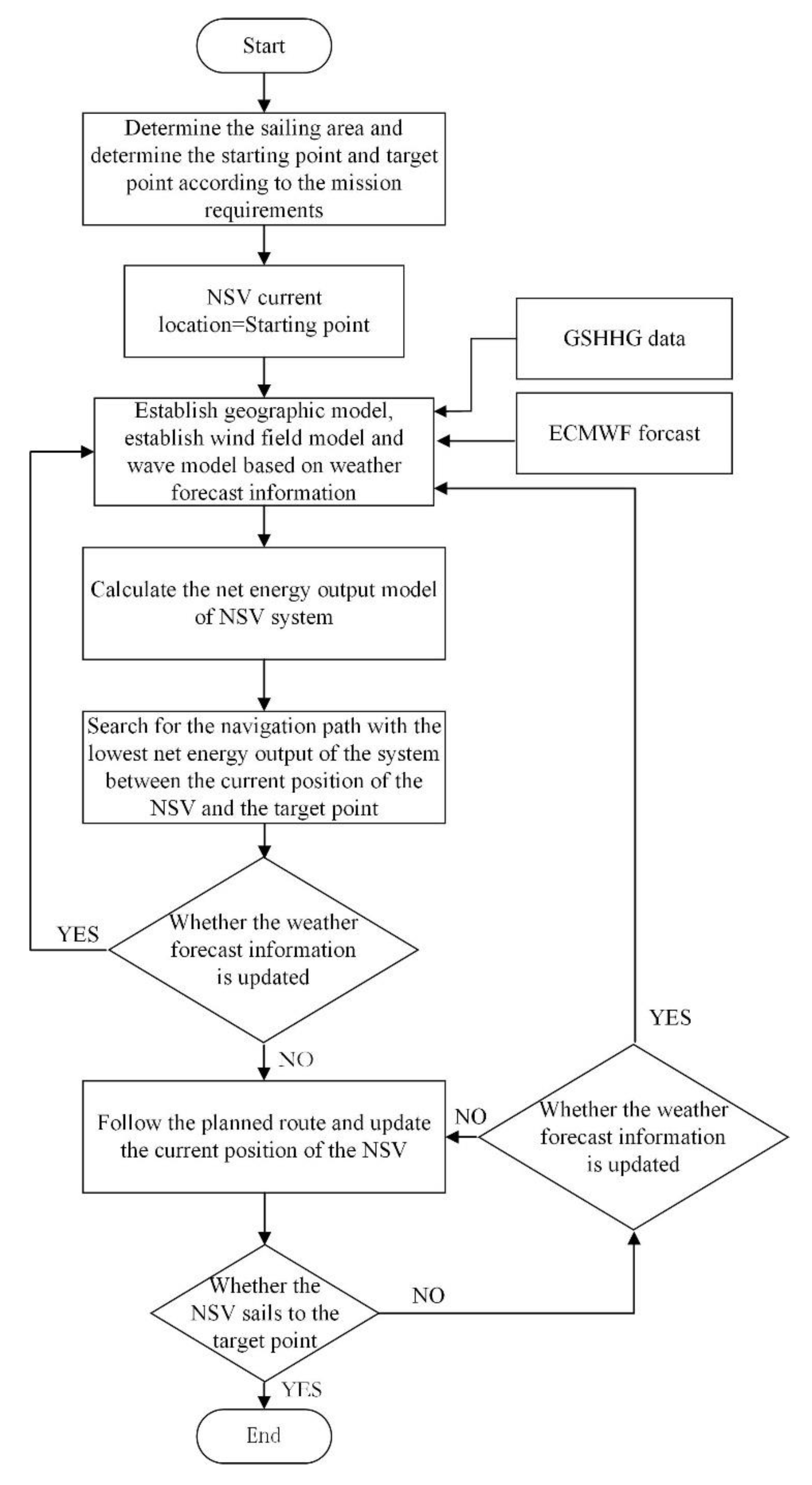
• The environment from the start point to the target point is dynamic so that the temporal and spatial variability of the offshore wind field needs to be taken into account when path planning.

The paper is organized as follows: In the current section, the literature on path planning considering wind effects is described, as well as the issues that need to be addressed in current research. How to solve problems 1 and 2 is dealt with in Section 2, and approaches to solving problems 3 and 4 are presented in the subsequent sections. Simulations and semi-physical simulations of the proposed method are carried out in Section 4 to verify its effectiveness. The work and analytical shortcomings of this paper are reviewed in Section 5, along with a discussion of future research. The conclusions of the current study are reported in the final section.

2. Offshore Wind Field Modeling and Wind Energy Capture Experiment

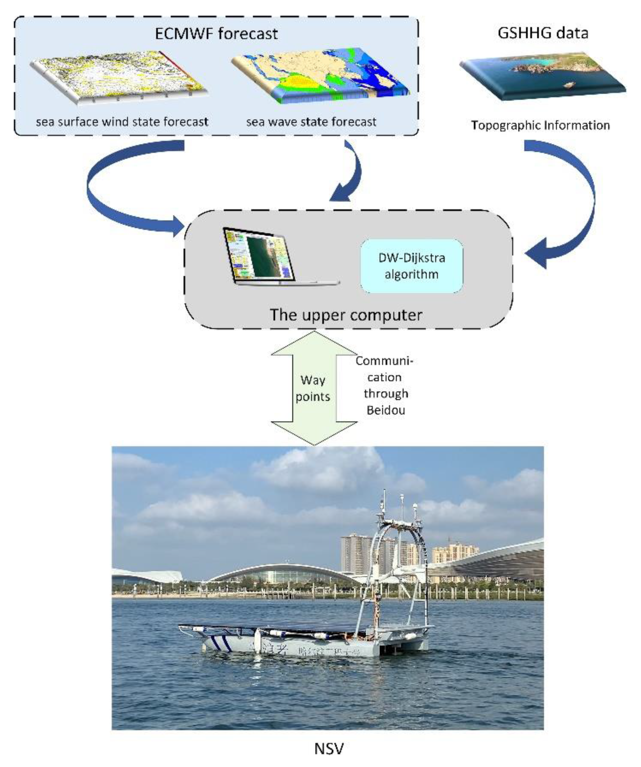
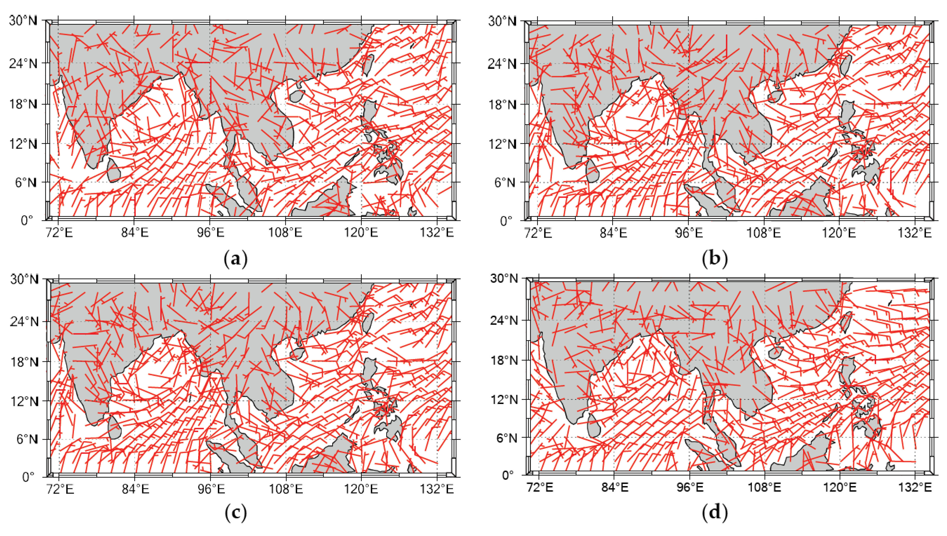
2.1. Time-Varying Ocean Wind Field Visualization Modeling

The representation methods of maps in robotics are divided into four categories, namely feature maps, topological maps, grid maps, and direct representation methods. The grid map, the map closest to human cognition, is the most common way for robots to describe the environment, which divides the environment into a series of grids. Each grid is given a possible value, which represents the probability that the grid is occupied. It was first proposed by NASA’s Alberto Elfes [31] in 1989 and was used on the Mars rover. The grid map is essentially a bitmap image, but each “pixel” represents the probability distribution of obstacles in the real environment. In this paper, a grid map is used to construct a global real ocean wind field environment.

The ocean and land modeling are divided into navigable and prohibited areas through coastline coordinates provided by a Global Self-Consistent, Hierarchical, High-resolution Geography Database (GSHHG) [32]. The data information of the ocean wind field calls the Atmospheric Model high resolution 10-day forecast data set [33], which comes from the European Centre for Medium-Range Weather Forecasts (ECMWF). The resolution of the topographic dataset is 0.04 degrees, and the resolution of the wind field dataset is 0.25 degrees. Assuming that both wind speed and wind direction are linear in space, the wind field data is double interpolated according to latitude and longitude to obtain an augmented wind field dataset with the same resolution as the topographic dataset. According to the information of the above data set, the time-varying modeling of the ocean wind field can be carried out, as shown in Figure 1.

Among them, the red wind vector, composed of a wind direction rod and a wind feather, indicates the size and direction of the wind. The wind direction rod points out the direction of the wind, while the wind feathers use long and short dashes, or combine with wind triangles, to indicate the size of the wind speed. From Figure 1, we can see that the wind speed and wind direction are changing at different locations or at different times. Therefore, the spatial-temporal variation characteristics of wind element information need to be considered when planning the path considering wind energy capture for the NSV.

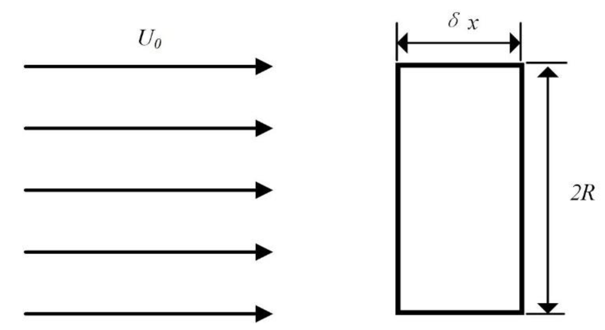
2.2. Airflow Power Density Model for Offshore Wind Field

Conventional marine vehicles usually only need to consider the consumption of the route to complete the search of the planned route; the NSV has a variety of marine energy capture devices that requires energy capture to be considered along with the length of the route. This paper only presents guidance on path planning for energy capture by wind energy capture devices, ignoring the impact of energy capture by other devices.

Based on the demand for wind energy capture, a grid model of offshore wind energy needs to be constructed. The variables appearing in this paper are explained in

Table A1. The name and meaning of the variable.

Variable Name	Variable Meaning
$A_{wind\_turbine}$	Wind turbine circular blade disk area
$R$	Wind turbine blade radius
$\rho$	Airflow density
$U_0$	Airflow velocity
$K$	The kinetic energy passing through the wind wheel
$P_{wind}$	Airflow power of offshore wind field
$P{D}_{wind}$	Airflow power density of offshore wind field
$P_{wind\_turbine}$	The energy power obtained by the wind energy capture system
$C_p$	Power coefficient
$C_p{}_1$	Power coefficient considering the conversion loss of kinetic energy produced by air to electric energy
$V_{wind\_a}$	Apparent wind
${\mathrm{V}}_{wind\_s}$	Ship wind
${\mathrm{V}}_{wind\_t}$	True wind
$P_{wind\_electricity}$	The energy input power of NSV
${\theta }_{wind}$	The angle between the apparent wind and the bow of NSV
$R_{wind}$	The longitudinal wind force on the NSV
$g$	Gravitational acceleration
$R_{wave}$	The longitudinal wave resistance of the NSV
$H$	Significant wave height
$L$	Average wavelength
$T$	Average wave period
${\theta }_{wave}$	The angle between the wave direction and the bow of the NSV
$F_t$	The thrust force generated by the NSV thruster
$P_e$	The average working power of each sensor and control system of NSV
$f_{FP}\left(x\right)$	Thruster power when thrust is $x$
$P_{total}$	The total output power of NSV
$E_{net\_consumption}$	The net energy consumption of NSV

. On the sea, the role of wind turbines is to convert the kinetic energy of wind into electrical energy. In this paper, airflow power density is used to describe the ocean wind field in a digitized manner. The variable $P{D}_{wind}$ is explained below by the Control Volume analysis method [34]. As shown in Figure 2, the wind turbine is represented as a circular blade disk with an area $A_{wind\_turbine}=\pi R^2$, where, $R$ is the radius of the blade and the unit is m. Viewing the rotating blade from the side, we abstract this part into a cuboid, which is the element volume of the airflow.

The element volume is the volume of an area element, that is, the product of the area $\Delta A_{wind\_turbine}$ and the length $\delta x$, so its mass is $\rho \Delta A_{wind\_turbine}\delta x$, $U_0$ is the airflow velocity, and the kinetic energy is $1/2\rho \Delta A_{wind\_turbine}\delta x{U}_0{}^2$. Considering the time $\delta t$ for the element to pass through the blade disc, $\delta x=U_0\delta t$ is obtained. The element’s contribution $\Delta KE$ to the total kinetic energy passed in time $\delta t$ is calculated by using (1):

$$\delta \left(\Delta KE\right)=\frac{1}{2}\rho \Delta A_{wind\_turbine}{U}_0\delta t{U}_0{}^2$$

(1)

The sum of the kinetic energy of all the elements that make up the wind wheel is the kinetic energy passing through the wind wheel. It was calculated by using (2):

$$\delta \left(KE\right)=\frac{1}{2}\rho A_{wind\_turbine}{U}_0{}^3\delta t$$

(2)

By calculating the limit $\left(\delta t\to 0\right)$ of the (2), we can get (3) [33,34]:

$$P_{wind}=\mathrm{d}\left(KE\right)/\mathrm{d}t=\frac{1}{2}\rho A_{wind\_turbine}{U}_0{}^3$$

(3)

where, $P_{wind}$ is power, and the unit is $\mathrm{W}$. To make the formula more universal, we can get the airflow power density of the offshore wind field without considering the blade parameters of the wind turbine, as shown in (4) [35,36]:

$$P{D}_{wind}=P_{wind}/A_{wind\_turbine}=\frac{1}{2}\rho U_0{}^3$$

(4)

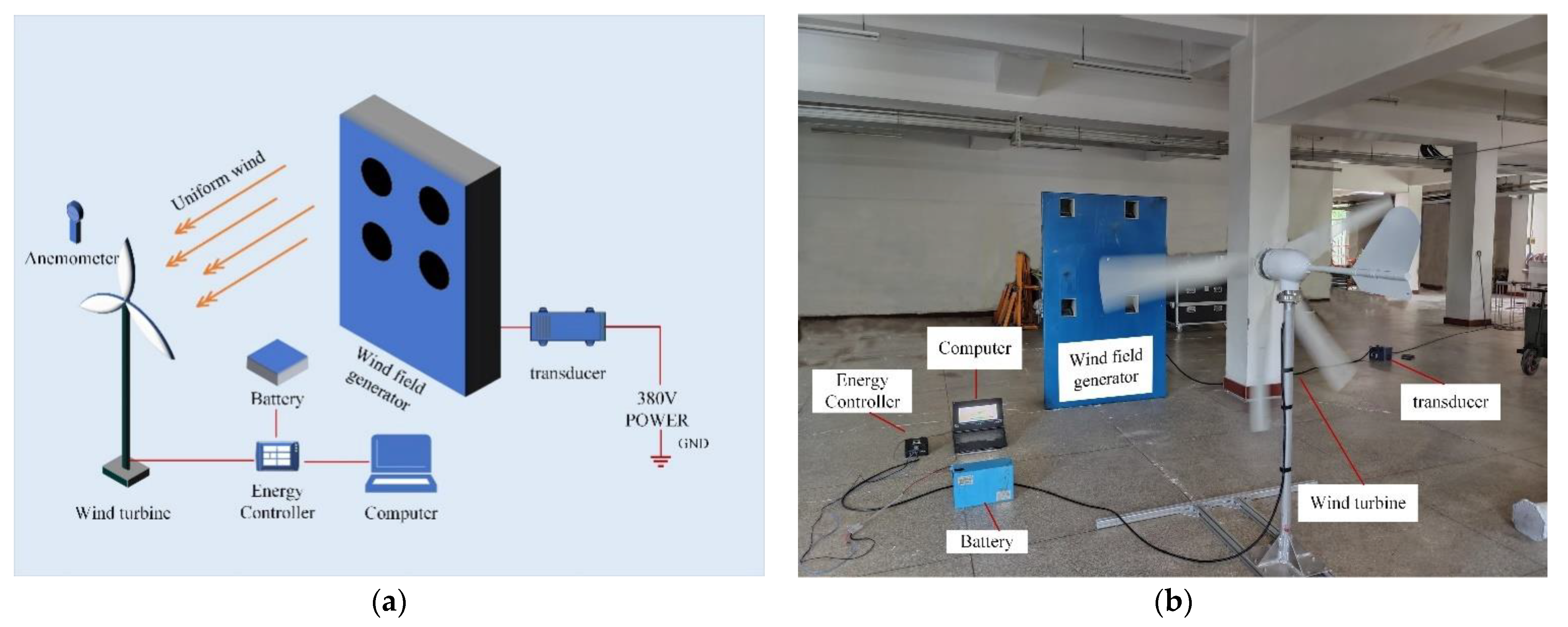
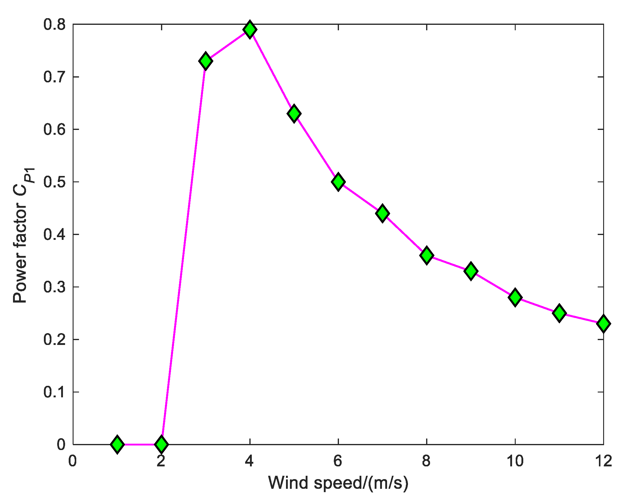
2.3. Wind Energy Capture Experiment

The wind energy capture system carried by the NSV uses a wind turbine to drive the wind turbine blades to rotate, and then the speed of rotation is increased by a speed increaser to promote the generator to generate electricity. Then the electric energy is stored in the battery through the NSV’s dedicated energy management equipment [37], as an energy supply for the NSV.

To obtain the efficiency of the transmission chain and the generator, and the aerodynamic loss of air retention, combined with (4), the energy power obtained by the wind energy capture system is calculated by (5):

$$P_{wind\_turbine}=C_p·P{D}_{wind}·A_{wind\_turbine}=C_p·\frac{1}{2}\rho U_0{}^3\pi R^2$$

(5)

where, $C_p$ is the ratio between the actual output power and the wind power passing through the blade disk, and it has no dimension.

We cannot obtain $C_p$ directly, but we can obtain $C_p{}_1$ by simulating wind field power generation experiments, $C_p{}_1=\eta ·C_p$, where, $\eta$ is the conversion coefficient. We designed the experiment shown in Figure 3 for the determination of $C_p{}_1$. The wind field generator is composed of four electric fans, and a uniform wind field of 0–12 m/s can be produced through a frequency converter. This experiment was completed in a closed room. Before the experiment, the wind speed in the room was measured with an anemometer, and the wind speed in the room was 0 m/s. After switching on the wind field generator, the wind speed is tested at the wind turbine experimental position until the desired wind speed is reached and stabilized by adjusting the transducer, then the wind turbine is allowed to start working. In the test, the wind turbine rotates under the action of the wind, and the energy controller transfers the electric energy converted from the wind turbine to the storage battery and forwards the power signal to the computer, which records the data.

Through the experiment, we got

Table 1. The power and power coefficient $C_p{}_1$ of the wind turbine at different wind speeds.

$\mathbf{Win}\mathbf{d} \mathbf{Speed}/ (\mathbf{m}/\mathbf{s})$	${\mathit{P}}_{\mathit{w}\mathit{i}\mathit{n}\mathit{d}\_\mathit{t}\mathit{u}\mathit{r}\mathit{b}\mathit{i}\mathit{n}\mathit{e}}\mathrm{/} \mathsf{W}$	${\mathit{C}}_{\mathit{P}1}$
1	0	0.00
2	0	0.00
3	28.62	0.73
4	72.48	0.79
5	112.84	0.63
6	154.73	0.50
7	218.46	0.44
8	269.36	0.36
9	345.82	0.33
10	402.33	0.28
11	473.29	0.25
12	572.81	0.23

and Figure 4.

According to Table 1, we can interpolate to obtain $C_p{}_1$ at different wind speeds, and then calculate the power generation of the wind energy capture system by (6):

$$\begin{array}{l}{P}_{wind\_electricity}=\eta ·C_p·P{D}_{wind}·A_{wind\_turbine}\\ =C_{p1}·\frac{1}{2}\rho U_0{}^3\pi R^2\end{array}$$

(6)

3. Design of Path Planning Method Considering Wind Energy Capture

3.1. Energy Input and Output Model of NSV System Considering Wind Energy Capture

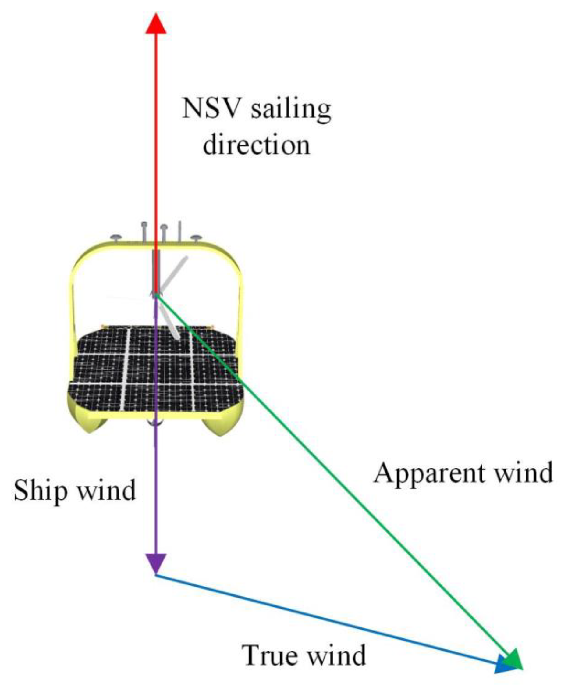
3.1.1. NSV System Energy Input Model

This article focuses on wind energy capture and does not consider the capture of other ocean energy (light radiation, ocean currents, etc.). Assuming that the capture of other ocean energy is zero, the total input of the NSV system is the electrical energy generated by the wind energy capture system. The NSV wind energy capture system is the same as the power generation equipment [37] used in the Section 2.3 wind energy capture experiment, consisting of a wind generator, an energy controller, and a battery. The wind turbine is mounted above the NSV deck. When the NSV is sailing, the power generation effect of the wind turbine is affected by the apparent wind, which is determined by the ship wind and the real wind, as shown in Figure 5.

The direction of the ship wind is opposite to the NSV course, and the magnitude is equal to the speed, while the true wind is the vector representation of the sea breeze relative to the earth coordinate system. The apparent wind is the wind observed on the NSV platform and can be calculated by (7). Therefore, even in an environment with a constant sea breeze, the amount of wind energy captured is affected by the heading and speed of the NSV:

$$V_{wind\_a}={\mathrm{V}}_{wind\_s}+{\mathrm{V}}_{wind\_t}$$

(7)

For a movable NSV, the $U_0$ in Section 2.3 should be corrected according to the NSV speed, that is, $U_0=\left|{\mathrm{V}}_{wind\_a}\right|$. Therefore, according to (6) and (7), the energy input power of the NSV is calculated by using (8):

$$P_{wind\_electricity}=C_{p1}·\frac{1}{2}\rho {\left|{\mathrm{V}}_{wind\_a}\right|}^3\pi R^2$$

(8)

3.1.2. NSV System Energy Output Model

Energy output refers to the energy consumption of the NSV navigating in the marine environment to ensure the normal operation of various sensors, control systems, and thrusters. In this article, we do not consider the impact of ocean currents on the speed of the NSV, but only consider the resistance of wind and waves to the hull of the NSV in the marine environment.

When the wind energy capture system is mounted on the NSV, as the wind speed increases, the NSV will capture more energy, but at the same time, the NSV faces greater wind resistance due to the increase in wind speed. The longitudinal force of the NSV under different wind speeds is calculated by CFD technology, and the longitudinal wind force on the NSV is calculated by using (9) [28]. Where, ${\theta }_{wind}\in \left(0,\pi \right)$ is the angle between the apparent wind and the bow of NSV:

$$R_{wind}=0.163·{\mathrm{V}}_{wind\_a}{}^2·\cos {\theta }_{wind}$$

(9)

With the influence of the sea surface wind field, the sea surface will also produce waves [38]. The wave forecast information is obtained through the date of significant wave height, mean wave period, and mean direction in ECMWF. Here, we simplify the ocean wave forecasting model, taking the significant wave height as the equivalent wave height in the NSV navigation area, and the average wave direction as the equivalent wave direction in the NSV navigation area. Using CFD technology, we calculated the NSV’s movement resistance in waves and obtained the wave resistance that changes with time by using (10)–(11) [38]:

$$\begin{array}{cc}{R}_{wave}=& \left[1715-1236·\cos \left(\frac{5t}{8\sqrt{L}}\right)+4736·\sin \left(\frac{5t}{8\sqrt{L}}\right)\right]\hfill \\ & ·\frac{H^2}{L}·V_{ship}{}^2·\cos {\theta }_{wave}\hfill \end{array}$$

(10)

$$L=0.87·\frac{g}{2\pi }{T}^2$$

(11)

where, ${\theta }_{wind}\in \left(0,\pi \right)$ is the angle between the wave direction and the bow of the NSV.

For the NSV to maintain a constant cruising speed in the ocean, the NSV’s propeller needs to output thrust to offset the resistance during navigation. Therefore, the thrust force was calculated by using (12):

$$F_t=R_{wind}+R_{wave}$$

(12)

To obtain the power of the thruster at different thrusts we carried out thrust tests and performed polynomial fitting. Thruster power was calculated by using (13) [28]:

$$f_{FP}\left(x\right)=1.15x^2+31.61x+13.5$$

(13)

The total output power of the NSV system can be calculated according to (14):

$$P_{total}=f_{FP}\left(F_t\right)+P_e$$

(14)

3.1.3. NSV System Energy Net Output Model

When the NSV conducts route planning, it must not only capture as much natural energy as possible but also consider its energy output. Therefore, the net energy output of the NSV system is an important measure when searching for a route. When the NSV is sailing at sea, its net energy consumption in a period can be obtained by (15):

$$E_{net\_consumption}={\displaystyle \mathsf{\int }\left(P_{total}-P_{wind\_electricity}\right)·}\mathrm{d}t$$

(15)

3.2. Dynamic Path Planning in A Time-Varying Wind Field Environment

Although the NSV is equipped with a multi-energy collection system that can efficiently use various natural energy sources such as solar energy, wind energy, wave energy, etc., the NSV still faces the following main problems when planning long-range routes: (1) The division of navigable and forbidden zones; (2) Spatial changes of the marine wind field environment; (3) Time changes of the marine wind field environment; (4) The trade-off between energy capture for long-range navigation and its energy consumption.

In response to question (1), we analyzed the coastline data of GSHHG and formatted the map as a raster space, with the abscissa as the longitude direction and the ordinate as the latitude direction. The land and islands are marked as 0 and treated as impassable areas, and oceans, straits, and rivers are marked as 1, and are regarded as navigable areas. In this way, the planning space of the route can be limited in the navigable area to ensure the safety of NSV navigation.

We will divide the grid space and add the wind field data predicted by ECMWF according to geographic coordinates. The wind direction and wind speed in each grid characterize the wind field status of this sea area and it is assumed that the wind field status in the same sea area is the same. The different wind characteristics of different grids can express the spatial changes of the marine wind field environment, while the wind direction and wind speed in the same grid also change with time. Assuming that the state of the ocean wind field is constant within a certain interval, the length of the time interval depends on the update interval of the forecast data. When new forecast data is received, the wind element information in the grid is also updated accordingly, so that the time change of the ocean wind field can be expressed. The above method solves problems (2) and (3).

The difficulty of problem (4) is that when the NSV is planning a path, the net energy output of the NSV in various marine wind field environments needs to be predicted. In other words, net energy output varies in time and space. To solve this problem, we propose the following solution, as shown in Figure 6. The navigation area is determined from the starting point of the navigation task and the navigation area is gridded. The resolution of the grid map and topographic dataset is consistent. The wind field dataset and wave field dataset are double-interpolated according to latitude and longitude to obtain an augmented wind field dataset and an augmented wave field dataset at the same resolution as the grid map. Then, based on the above data, the weights of each grid are calculated using Equation (15), in which the wind data and wave data are merged into energy data. Finally, the route search is carried out on the upper computer using the DW–Dijkstra algorithm, and the planned waypoints are sent to the NSV via Beidou communication immediately. Once weather forecast information updates, the above steps are repeated.

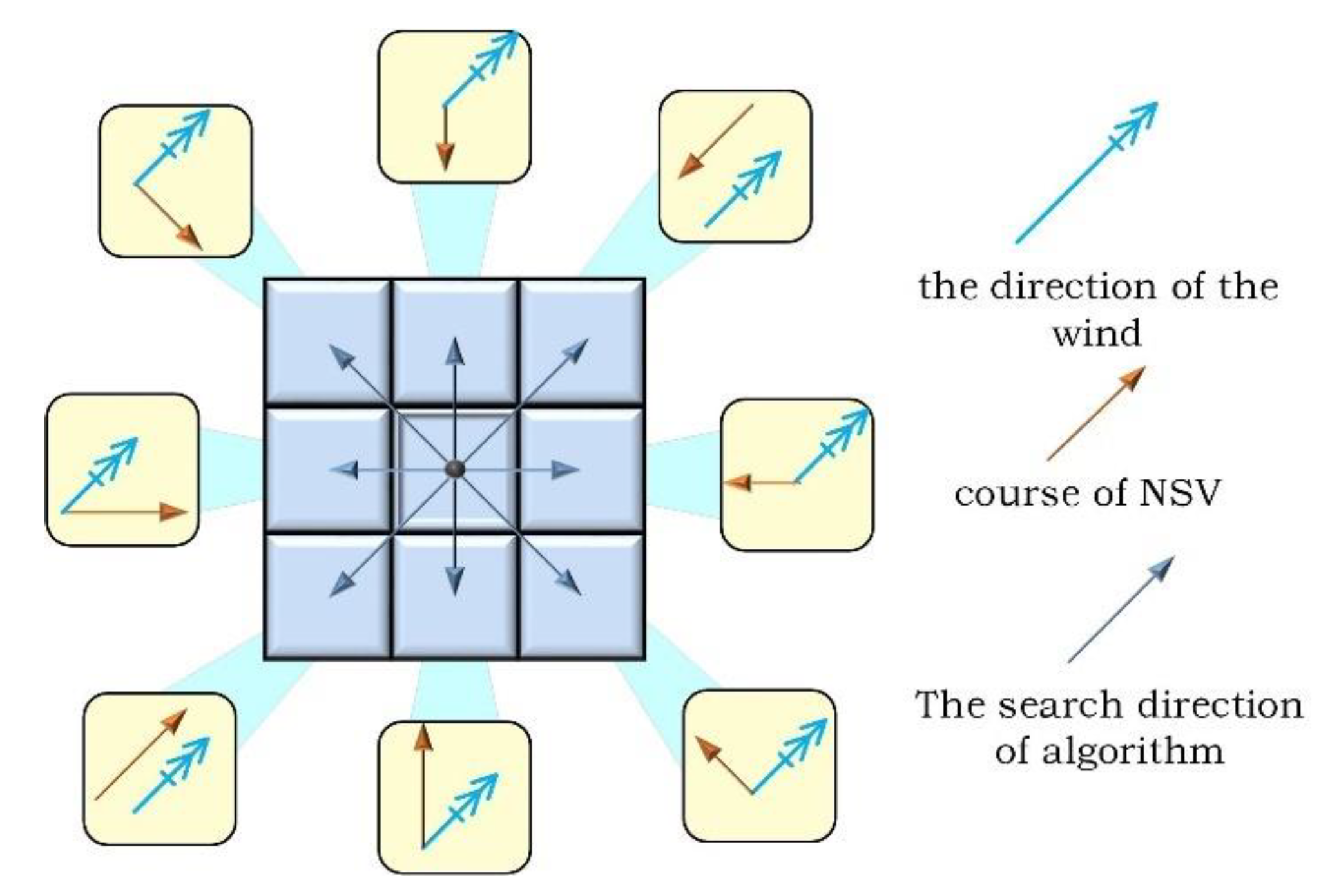
3.3. DW–Dijkstra Algorithm Design

The Dijkstra algorithm is a common algorithm graph for finding the shortest path in the graph theory proposed by Dutch computer scientist E.W. Dijkstra in 1959 [39]. It is suitable for single-source shortest path planning, that is, finding the shortest path from a point to any other vertex in the graph. According to the navigation characteristics of NSV and wind energy capture requirements, the DW–Dijkstra algorithm considering wind capture is proposed in this paper based on the Dijkstra algorithm.

The flow chart of this algorithm to solve NSV long-endurance dynamic path planning is shown in Figure 7. First, it is necessary to determine the navigation area, starting point, and target point according to the mission requirements, and establish a geographic model by calling GSHHG data. The wind field model and wave model are established by obtaining the forecast information of ECMWF and the net output model of the NSV system is calculated. According to the above model, the navigation path with the lowest net energy output of the system is searched from the current position of the NSV to the target point. Then the ECMWF forecast information is updated, the above steps will be used to re-plan the path until the target point is reached.

The pseudo-code of the DW–Dijkstra algorithm is shown in Algorithm 1. First, it is necessary to determine the starting point and target point of the planned task, as well as the current sea state information. Based on formula (15) in Section 3.1.3, $E_{net}$ ( ) can be calculated, and the path with the minimum $E_{net\_consumption}$ can be searched from the mission target point to the start point. Since it is searching backward from the target point, when calculating $c\left(X_n,X_i\right)$ of energy consumption between nodes, it should be noted that the navigation direction of the NSV is opposite to the search direction, and the calculation of ship wind should consider the direction, as shown in Figure 8.

When the sea state information is updated, the $S_{wind}{}_{\left(t\right)}$ and $S_{wave}{}_{\left(t\right)}$ are updated, and the path with the minimum $E_{net\_consumption}$ is re-searched from the mission target point to the current node of the NSV until the NSV sails to the mission target point.

Algorithm 1: DW–Dijkstra algorithm pseudo code.
Input: start node${\mathit{X}}_{local}$, end node${\mathit{X}}_{goal}$
1.	while Sea state is change do
2.	${\mathit{X}}_{end}$ = ${\mathit{X}}_{goal}$, ${\mathit{X}}_{start}$ = ${\mathit{X}}_{local}$, update $S_{wind}{}_{\left(t\right)}$, $S_{wave}{}_{\left(t\right)}$, Path_search( )
3.	function Path_list = Path_search(${\mathit{X}}_{start}$, ${\mathit{X}}_{end}$, $S_{wind}{}_{\left(t\right)}$, $S_{wave}{}_{\left(t\right)}$)
4.	According to the forecast define: wind state$S_{wind}{}_{\left(t\right)}$( ), wave state$S_{wave}{}_{\left(t\right)}$( )
5.	OPEN_list:= ${\mathit{X}}_{end}$, where $E_{net}\left({\mathit{X}}_{end},S_{wind\left(t\right)}\left({\mathrm{X}}_{end}\right),S_{wave}{}_{\left(t\right)}\left({\mathrm{X}}_{end}\right)\right)=0$
6.	CLOSE_list:= { }
7.	while  OPEN_list is not empty do
8.	current node ${\mathit{X}}_n$:= the node in the OPEN_list with the lowest   $E_{net}\left(\mathit{X},S_{wind\left(t\right)}\left(\mathit{X}\right),S_{wave\left(t\right)}\left(\mathit{X}\right)\right)$
9.	if  ${\mathit{X}}_n={\mathit{X}}_{start}$ break
10.	Remove ${\mathit{X}}_n$ from OPEN_list and add it to CLOSE_list
11.	for    each adjacent node, ${\mathit{X}}_i$ of ${\mathit{X}}_n$ do
12.	if $E_{net}\left({\mathit{X}}_i,S_{wind\left(t\right)}\left({\mathit{X}}_i\right),S_{wave\left(t\right)}\left({\mathit{X}}_i\right)\right)=0$‖${\mathit{X}}_i\in$ CLOSE_list continue
13.	if ${\mathit{X}}_i\notin$ OPEN_list
14.	add ${\mathit{X}}_i$ into OPEN_list
15.	the parent node of ${\mathit{X}}_i$, ${\mathit{X}}_{i\cdot parent}={\mathit{X}}_n$
16.	calculate $E_{net}\left({\mathit{X}}_i,S_{wind\left(t\right)}\left({\mathit{X}}_i\right),S_{wave\left(t\right)}\left({\mathit{X}}_i\right)\right)$
17.	if ${\mathit{X}}_i\in$ OPEN_list
18.	$E_{net}\left({\mathit{X}}_i,S_{wind\left(t\right)}\left({\mathit{X}}_i\right),S_{wave\left(t\right)}\left({\mathit{X}}_i\right)\right)\text{'}=E_{net}\left({\mathit{X}}_i,S_{wind\left(t\right)}\left({\mathit{X}}_i\right),S_{wave\left(t\right)}\left({\mathit{X}}_i\right)\right)$       $+c\left({\mathit{X}}_n,{\mathit{X}}_i\right)$
19.	if      $E_{net}\left({\mathit{X}}_i,S_{wind\left(t\right)}\left({\mathit{X}}_i\right),S_{wave\left(t\right)}\left({\mathit{X}}_i\right)\right)\text{'}\ge E_{net}\left({\mathit{X}}_i,S_{wind\left(t\right)}\left({\mathit{X}}_i\right),S_{wave\left(t\right)}\left({\mathit{X}}_i\right)\right)$ continue
20.	else
21.	${\mathit{X}}_{i\cdot parent}={\mathit{X}}_n$         $E_{net}\left({\mathit{X}}_i,S_{wind\left(t\right)}\left({\mathit{X}}_i\right),S_{wave\left(t\right)}\left({\mathit{X}}_i\right)\right)$         $=E_{net}\left({\mathit{X}}_i,S_{wind\left(t\right)}\left({\mathit{X}}_i\right),S_{wave\left(t\right)}\left({\mathit{X}}_i\right)\right)\text{'}$
22.	Resort and keep OPEN_list sorted by $E_{net}$ values
23.	${\mathit{X}}_P={\mathit{X}}_{end}$
24.	Path_list: =${\mathit{X}}_P$
25.	While  ${\mathit{X}}_p\ne {\mathit{X}}_{start}$ do
26.	${\mathit{X}}_p={\mathit{X}}_{p\cdot parent}$
27.	Path_list={Path_list,${\mathit{X}}_p$}
28.	flip(Path_list)
29.	Return: Path_list

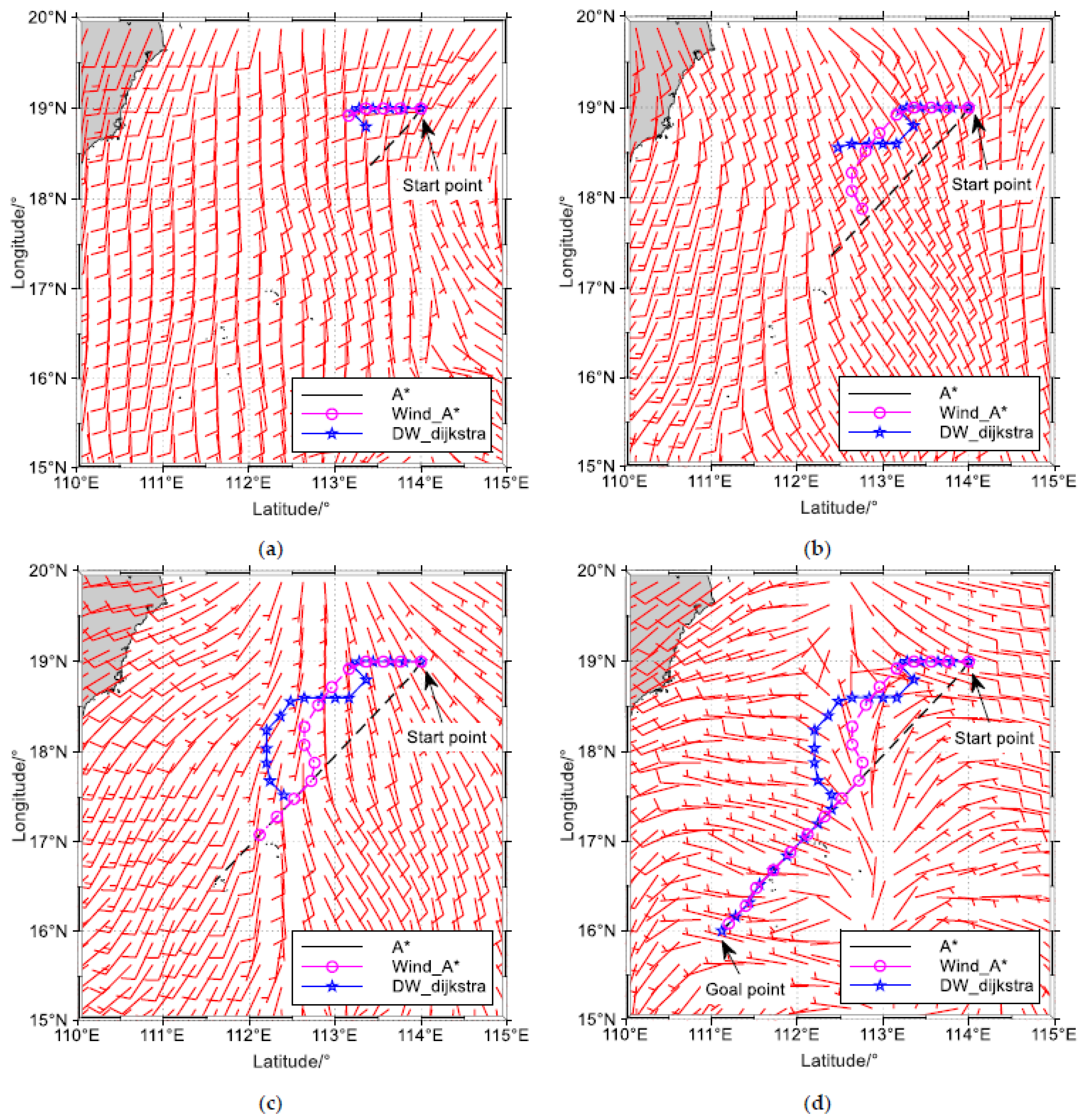
4. Algorithm Comparison Simulation Research

The proposed approach is simulated using Python 3.6 and Matplotlib 2.2.2. All simulations are performed on a PC with Microsoft Windows 10 as OS with Intel i7 2.50 GHz quad-core CPU and 16 GB RAM.

The hardware parameters of the energy capture system and output system of the NSV have been specially designed to meet the long endurance navigation requirements. After repeated measurements and tests, 1.5 m/s is the cruising speed that can maintain the NSV’s long-endurance. Therefore, the simulations set the cruise speed of the NSV as 1.5 m/s and carried out simulations to verify the artificial time-varying wind field environment and the real time-varying wind field environment, respectively.

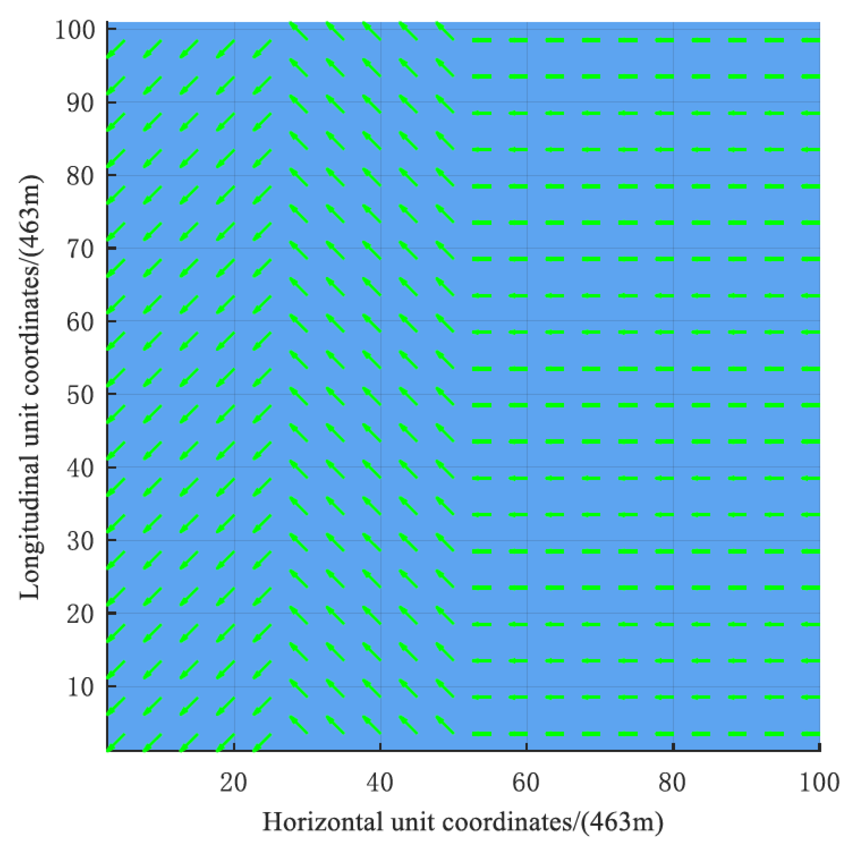
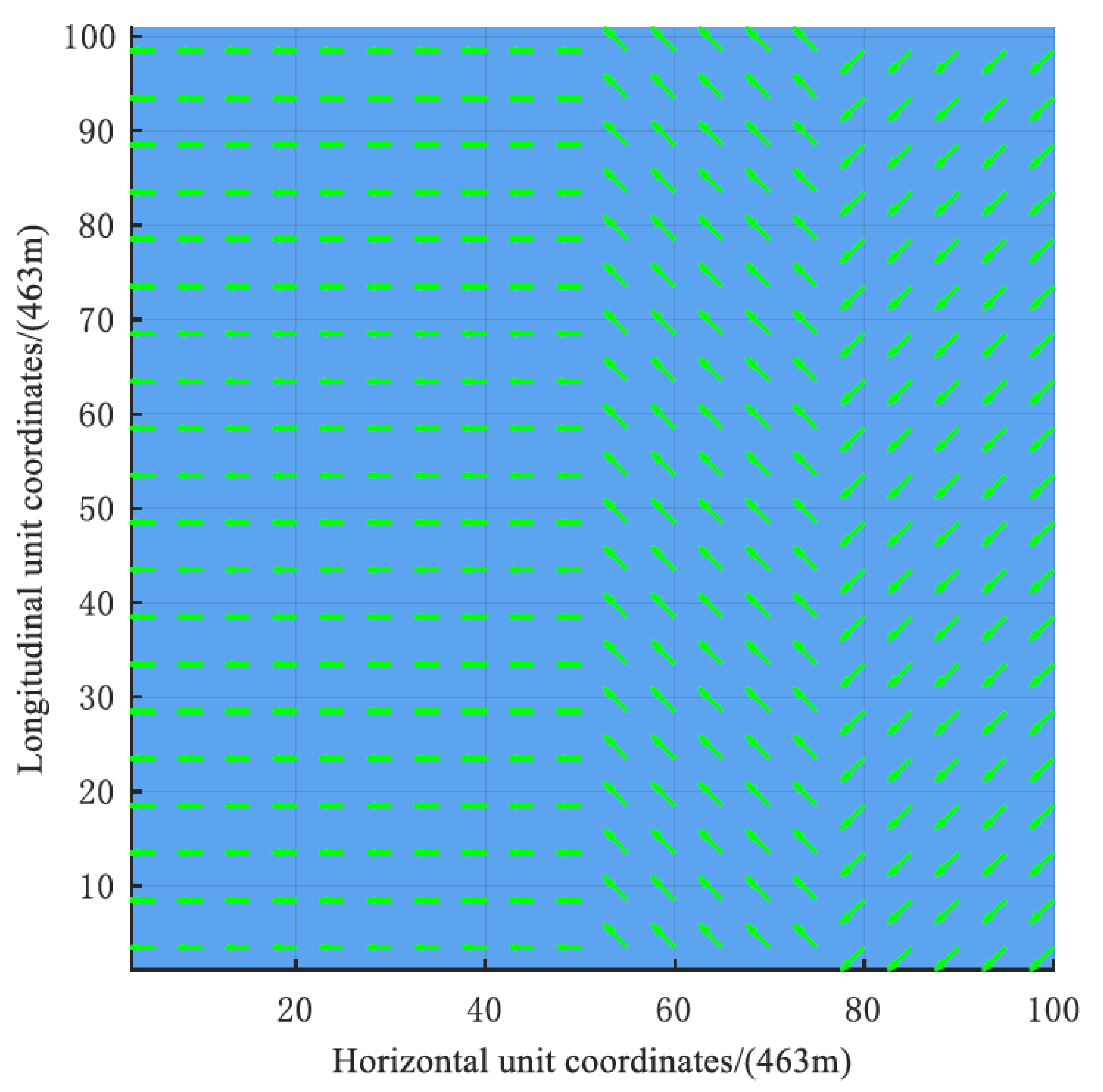
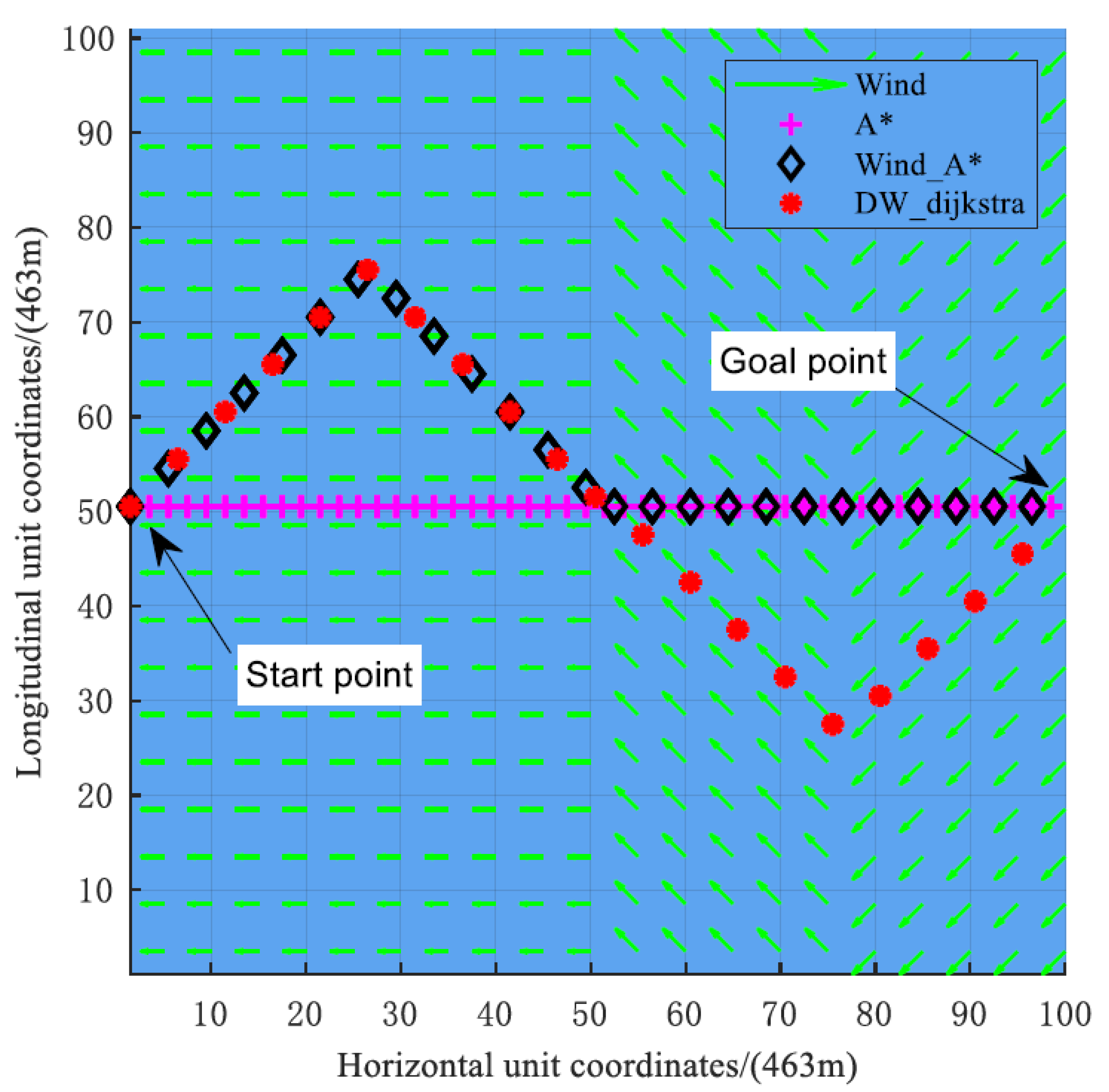
4.1. Simulation Comparison of Artificial Time-Varying Wind Field Environment

The artificial time-varying wind field environment simulation is based on a grid map with a grid resolution of 100 × 100. The unit distance of each grid is 463 m. The design navigation sea condition of the NSV is class 1–4.

According to the Beaufort scale definition [38], the wind speed can be set at 7 m/s for the fourth-level sea state, and the corresponding significant wave height in open ocean areas is 1.7 m, and the wave period is 5.6 s–6.1 s. In this simulation example, it is assumed that the wave period is 6 s, and the wave direction is opposite to the wind direction.

The wind direction and the changing state of the wind direction are shown in Figure 9; Figure 10. The update frequency of the wind state is 6 h, and the wind state in each period is constant by default.

The starting point position of the NSV is (1, 50), and the target point position is (100, 50). To test the effectiveness of the DW–Dijkstra algorithm, the energy consumption of the planned route is compared with the traditional A* algorithm and the Wind_A* algorithm. The results are shown as follows: Figure 11 shows the path diagrams of different algorithms, and

Table 2. Comparison of simulation energy consumption of three algorithms in an artificial wind field.

Algorithm Name	Energy Consumption/MJ	Energy Difference With A* Algorithm/MJ	Save Energy Compared to A* Algorithm/%
A* algorithm	2.23	-	-
Wind_A* algorithm	1.46	0.77	34.62
DW–Dijkstra algorithm	1.33	0.91	40.61

is the simulation energy consumption data comparison of different algorithms.

Figure 11 shows the paths planned by the three algorithms. Although the picture only shows the state of the wind field at the time ${\tau }_2$, it is a dynamic process. The state of the wind field changes from Figure 9 to Figure 10. Since the traditional A* algorithm does not consider the acquisition of energy, its planned route is not affected by either the spatial or temporal changes of the environment, so that it consumes the most energy; Wind_A* algorithm considers the capture of wind energy, it can respond to the spatial change of the wind field state at ${\tau }_1$, and save 34.62% of energy consumption compared with the traditional A* algorithm. The DW–Dijkstra algorithm considers not only the capture of wind energy but also the temporal and spatial changes of the wind field state so that it can effectively respond to the time change from the wind field state at ${\tau }_1$ to the wind field state at ${\tau }_2$. Compared with the traditional A* algorithm, the energy consumption is reduced by 40.61%, and the energy consumption is reduced by 9.16% compared with the Wind_A* algorithm.

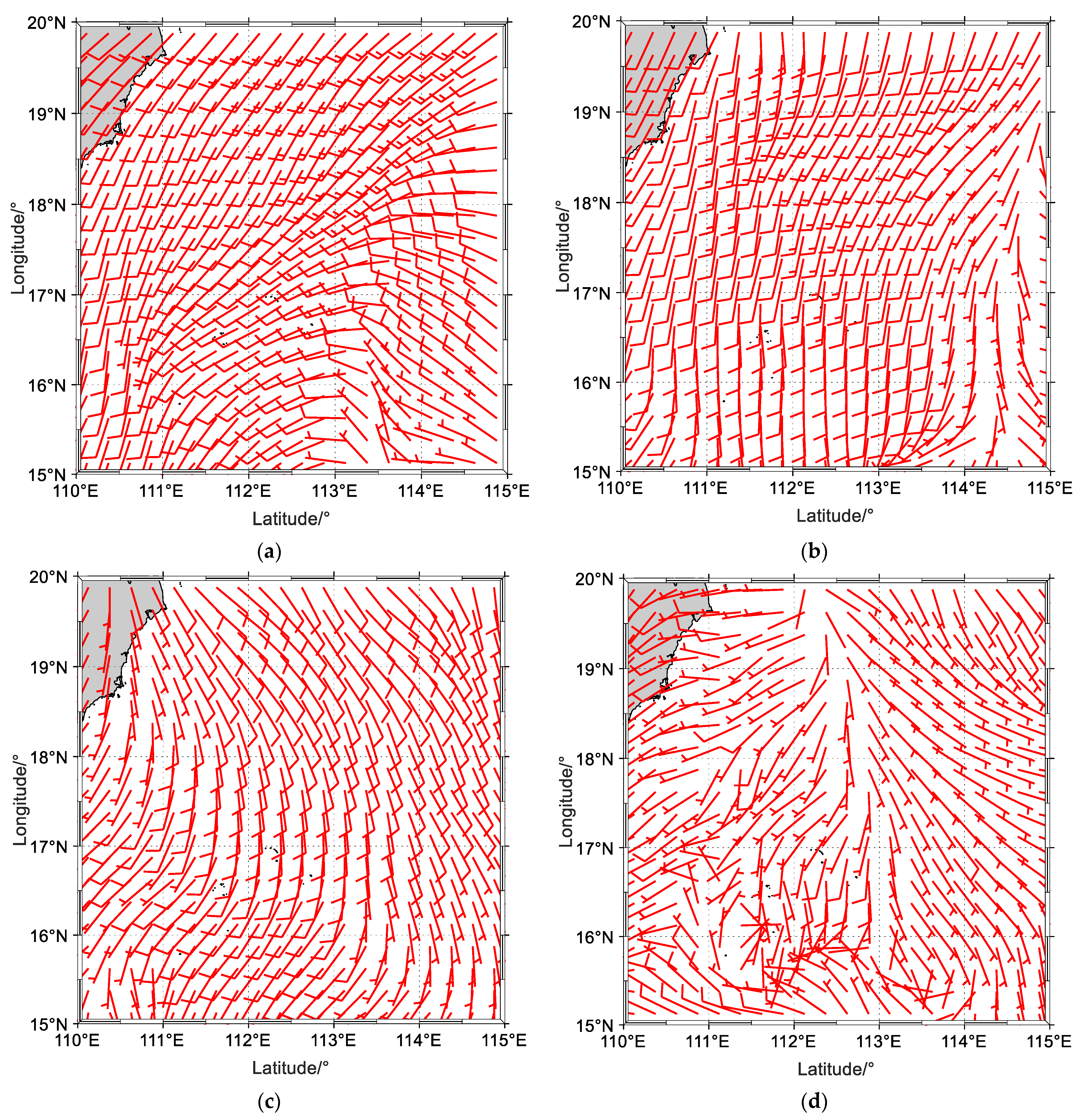
4.2. Semi-Physical Simulation Comparison of Real Time-Varying Wind Field Environment

The semi-physical simulation of the real-time-varying wind field environment is established in the southern China seas of 110° E–115° E, 15° N–20° N. The meteorological information of wind and waves comes from the fifth generation ECMWF re-analysis for the global climate and weather for the past four to seven decades (ECMWF’s ERA5) [40]. Assuming that the forecast information is unbiased and the state of the wind field in the forecast interval is constant, we use this data as the forecast data obtained by the NSV for the semi-physical simulation of the long-range dynamic path planning. Figure 12 shows the wind field model from 6 June 2021 to 9 June 2021. Each day is drawn at 00:00, corresponding to (a), (b), (c), and (d).

As shown in the figures below, the wind conditions in the southern seas of China have changed significantly in the four days.

The starting point of the NSV is 19° N, 114° E, and the target location is 16° N, 111° E. To test the effectiveness of the DW–Dijkstra algorithm, the energy consumption of the planned route is compared with the traditional A* algorithm and the Wind_A* algorithm.

The results are shown as follows: Figure 13 shows the path diagrams of different algorithms, where (a), (b), (c), and (d) correspond to 18:00 in the four days from June 6, 2021 to 9 June 2021 of the trajectory planned by three algorithms.

Table 3. Comparison of energy consumption of three algorithms in a real wind field.

Algorithm Name	Energy Consumption/MJ	Energy Difference with A* Algorithm/MJ	Save energy Compared to A* Algorithm/%
A* algorithm	81.79	-	-
Wind_A* algorithm	74.05	7.74	9.46
DW–Dijkstra algorithm	69.24	12.55	15.34

is the energy consumption data of the semi-physical simulation.

The traditional A* algorithm does not consider the capture of wind energy and directly plans the shortest route between the starting point and the target point. The Wind_A* algorithm considers the capture of wind energy but does not consider the time change of the wind field, so the path planned later cannot change with the change of the wind state. In the early stage, the wind state and planned path calculated by the DW–Dijkstra algorithm or Wind_A* algorithm is the same, but as the wind state changes with time, the path planned by the DW–Dijkstra algorithm also changes.

Compared with the traditional A* algorithm, Wind_A* algorithm and DW–Dijkstra algorithm save energy by 9.64% and 15.07% respectively.

5. Discussion

In this paper, a time-varying ocean wind field environment visualization model for NSV path planning and an offshore wind field airflow power density model are constructed based on ocean weather forecast data from ECMWF and the GSHHG coastline dataset. The $C_p{}_1$ was calibrated through wind energy capture experiments and a mapping between the offshore wind speed and the electricity captured by the wind turbine was obtained. The energy input and output model of the NSV system are constructed based on the wind catching characteristics of the NSV, the wave response, and the energy consumption of the onboard equipment [41].

Based on the net energy output model of the NSV system, the weight function of Dijkstra’s algorithm is modified to adapt to the spatial and temporal variability of the dynamic ocean wind field, and the DW–Dijkstra algorithm is proposed. The DW–Dijkstra algorithm saves 40.61% energy compared to the traditional A* algorithm and 9.16% compared to the Wind_A* algorithm in the simulation. In the semi-physical simulation, the DW–Dijkstra algorithm can save 15.07% compared to the traditional A* algorithm and 6.50% compared to the Wind_A* algorithm. The results in Section 4.2 show a decrease in energy savings compared to the results in Section 4.1, which can be attributed to the following. (1) The wind speed in the real wind field is small, between 2 m/s–5 m/s, resulting in low capturable wind energy at sea. (2) The wind direction change in the real wind field is not as drastic as the change in the artificial wind field. Although the wind speed in the real wind field is small and the wind direction change is not as obvious as that in the artificial wind field, the DW–Dijkstra algorithm can still plan the route with the lowest energy consumption among the three algorithms, which verifies its effectiveness.

The calculation results of the NSV system energy input model can lead to model bias due to the following. (1) The wind dataset used in the algorithm only provides data information at a height of 10 m above the sea surface, while the NSV’s wind turbine is 1.7 m above the sea surface. (2) In addition to the yaw altering the apparent wind, the NSV’s continuous roll and pitch also cause bias in the apparent wind calculation. (3) Vibration of the wind turbine structure caused by attitude changes can also affect the conversion efficiency. These are also the gaps between the semi-physical simulations and experiments in real marine environments.

The method proposed in this paper is large-scale route planning method with a minimum interval of 0.04 degrees between waypoints, which can meet the needs of NSVs navigating over large oceans, ensure the NSV can stay away from large islands and coastlines, and provide a long-range route guidance for NSVs considering wind energy capture. However, it does not meet the fine-scale navigation needs of NSVs (e.g., in ports, waterways) and further research is needed on small and medium-scale path planning methods.

6. Conclusions

In this paper, a long-endurance dynamic path planning method for the NSV considering wind energy capture is proposed. This method was validated by simulation in an artificial time-varying wind field environment. The method was validated by semi-physical simulations in a realistic time-varying wind field environment by calling meteorological data of the southern Chinese waters. The results show that the DW–Dijkstra algorithm can effectively respond to the spatial and temporal variations of both wind fields. While compared with the A* and wind_A* algorithms, this method can plan the navigation path with the lowest net energy output of the system and effectively increase the endurance of the NSV.

Future research should focus on improving the search efficiency of the algorithm, which can be used to overcome the disadvantage of the algorithm requiring multiple searches to complete the pathfinding. In addition, the NSV can carry a variety of energy capture devices, and the coupling effects of combined energy capture by multiple devices on route planning also requires further study.

References

1. Xu, P.F.; Cheng, C.; Cheng, H.X. Identification-based 3 DOF model of unmanned surface vehicle using support vector machines enhanced by cuckoo search algorithm. Ocean Eng. 2020, 197, 1–11. [Google Scholar] [CrossRef]
2. Peng, Z.H.; Wang, J.; Wang, D. An overview of recent advances in coordinated control of multiple autonomous surface vehicles. IEEE Trans. Ind. Inform. 2020, 17, 732–745. [Google Scholar] [CrossRef]
3. Zheng, C.W.; Pan, J. Assessment of the global ocean wind energy resource. Renew. Sustain. Energy Rev. 2014, 33, 382–391. [Google Scholar] [CrossRef]
4. Rynne, P.F.; Ellenrieder, K.D.V. Unmanned Autonomous Sailing: Current Status and Future Role in Sustained Ocean Observations. Mar. Technol. Soc. J. 2009, 43, 21–30. [Google Scholar] [CrossRef]
5. Yu, J.C.; Sun, Z.Y.; Zhang, A.Q. The Present Status of Environmental Energy Harvesting and Utilization Technology of marine Robots. Robot 2018, 40, 91–103. [Google Scholar]
6. Rynne, P.F.; Von Ellenrieder, K.D. A Wind and Solar-Powered Autonomous Surface Vehicle for Sea Surface Measurements; OCEANS: Piscataway, NJ, USA, 2008; pp. 2110–2115. [Google Scholar]
7. ELKAIMGH. System Identification for Precision Control of a Wing Sailed GPS-Guided Catamaran. Ph.D. Thesis, Stanford University, Stanford, CA, USA, 2002.
8. HWT X-3 Production Vessel Design. Available online: http://www.harborwingtech.com/HWT-X-3-Production-Design.htm (accessed on 29 December 2017).
9. Submaran™ S10: Wind and Solar-Powered Freedom to go Further and Faster. Available online: http://www.oceanaero.us/Ocean-Aero-Submaran (accessed on 22 October 2017).
10. Hook, D.; Daltry, R.; Coelho, R. C-Enduro USV Developed for Offshore Long-Endurance Appllications ASV Designs Vehicle for UK NOC’s LEMUSV Concept. Sea Technol. 2014, 55, 15–17. [Google Scholar]
11. Jiang, Q.Q.; Li, K.; Liao, Y.L. Model-free Adaptive Speed Control Method of Natural Energy-driven Unmanned Surface Vehicle. Unmanned Syst. Technol. 2020, 3, 37–42. [Google Scholar]
12. You, X.; Ma, F.; Huang, M. Study on the MMG three-degree-of-freedom motion model of a sailing vessel. In Proceedings of the 2017 4th International Conference on Transportation Information and Safety (ICTIS), Banff, AB, Canada, 8–10 August 2017; pp. 395–399. [Google Scholar]
13. Luo, X. Conception Researchand Validation of Intelligent Green Autonomous Sailboat. Ph.D. Thesis, Shanghai Jiao Tong University, Shanghai, China, 2017. [Google Scholar]
14. Ma, B.Y. Study on Surface Sailing Characteristics of the Wind Powered Vehicle with Deployable/Foldable Wing Sail. Ph.D. Thesis, Tianjin University, Tianjin, China, 2018. [Google Scholar]
15. Zhang, H.N. Automatic Generation and Path Planning of Unmanned Boat Routes Based on Ant Colony Optimization Algorithm. Ship Electron. Eng. 2019, 39, 46–49, 97. [Google Scholar]
16. Mousazadeh, H.; Kiapey, A. Experimental Evaluation of a New Developed Algorithm for An Autonomous Surface Vehicle and Comparison with Simulink Results. China Ocean Eng. 2019, 33, 268–278. [Google Scholar] [CrossRef]
17. Paravisi, M.; Santos, D.H.; Jorge, V. Unmanned Surface Vehicle Simulator with Realistic Environmental Disturbances. Sensors 2019, 19, 68. [Google Scholar] [CrossRef] [Green Version]
18. Dos, S.D.H.; Goncalves, L.M.G. A gain-scheduling control strategy and short-term path optimization with genetic algorithm for autonomous navigation of a sailboat robot. Int. J. Adv. Robot. Syst. 2019, 16, 1–15. [Google Scholar]
19. Du, M.S.; Xu, J.S. Study of Long-term Route Planning for Autonomous Sailboat. Ship Eng. 2018, 40, 11–14, 88. [Google Scholar]
20. Andouglas, G.D.S.J.; Santos, D.H.D.; Negreiros, A.P.F.D. High-Level Path Planning for an Autonomous Sailboat Robot Using Q-Learning. Sensors 2020, 20, 1550–1571. [Google Scholar]
21. Yu, J.C.; Sun, Z.Y.; Zhang, A.Q. Research Status and Prospect of Autonomous Sailboats. J. Mech. Eng. 2018, 54, 112–124. [Google Scholar] [CrossRef]
22. Niu, H.L.; Lu, Y.; Savvaris, A. Efficient Path Planning Algorithms for Unmanned Surface Vehicle. IFAC Pap. 2016, 49, 121–126. [Google Scholar] [CrossRef]
23. Niu, H.L.; Ji, Z.; Savvaris, A. Energy efficient path planning for Unmanned Surface Vehicle in spatially-temporally variant environment. Ocean Eng. 2020, 196, 106766. [Google Scholar] [CrossRef]
24. Song, R.; Liu, Y.; Bucknall, R. A multi-layered fast marching method for unmanned surface vehicle path planning in a time-variant maritime environment. Ocean Eng. 2017, 129, 301–317. [Google Scholar] [CrossRef]
25. Singh, Y.; Sharma, S.; Sutton, R. Optimal path planning of an unmanned surface vehicle in a real-time marine environment using a Dijkstra algorithm. Marine Navigation. In Proceedings of the International Conference on Marine Navigation and Safety of Sea Transportation, Gdynia, Poland, 21–23 June 2017; Weintrit, A., Ed.; CRC Press/Balkema: Plymouth, UK, 2017; pp. 399–402. [Google Scholar]
26. Singh, Y.; Sharma, S.; Sutton, R. A constrained A* approach towards optimal path planning for an unmanned surface vehicle in a maritime environment containing dynamic obstacles and ocean currents. Ocean Eng. 2018, 169, 187–201. [Google Scholar] [CrossRef] [Green Version]
27. Jia, Q.; Liao, Y.L.; Pang, S. Route Planning Method of Natural Energy Driven Unmanned Surface Vehicle Considering Wind Energy Capture. China Patent 2020111040258, 15 October 2020. [Google Scholar]
28. Jia, Q.; Liao, Y.L.; Pang, S. NSV long endurance path planning method considering wind energy capture. J. Cent. South Univ. (Nat. Sci. Ed.). in press.
29. Liang, X.; Li, L.; Wu, J. Mobile robot path planning based on adaptive bacterial foraging algorithm. J. Cent. South Univ. 2013, 20, 3391–3400. [Google Scholar] [CrossRef]
30. Raja, P.; Abhilash, M.; Ravi Shanker, K. Quadrant based incremental planning for mobile robots. J. Cent. South Univ. 2014, 21, 1792–1803. [Google Scholar] [CrossRef]
31. Elfes, A. Using occupancy grids for mobile robot perception and navigation. Computer 1989, 22, 46–57. [Google Scholar] [CrossRef]
32. A Global Self-Consistent, Hierarchical, High-Resolution Geography Database(GSHHG). Available online: http://www.soest.hawaii.edu/wessel/gshhg/ (accessed on 15 June 2017).
33. Atmospheric Model High Resolution 10-Day Forecast (Set I-HRES). Available online: https://www.ecmwf.int/en/forecasts/dataset/atmospheric-model-high-resolution-10-day-forecast (accessed on 12 May 2021).
34. Wood, D. Small Wind Turbines: Analysis, Design, and Application; Springer: Berlin, Germany, 2011; pp. 1–29. [Google Scholar]
35. Burton, T.; Sharpe, D.; Jenkins, N. Wind Energy Handbook; John Wiley & Sons: Chichester, UK, 2001; pp. 11–39. [Google Scholar]
36. Manwell, J.; McGowan, J.; Rogers, A. Wind Energy Explained: Theory, Design and Application; John Wiley & Sons: New York, NY, USA, 2002; pp. 83–140. [Google Scholar]
37. The NSV Wind Energy Capture System; Science and Technology on Underwater Vehicle Laboratory, Harbin Engineering University: Harbin, China, 2021.
38. Wen, S.C.; Yu, Z.W. Ocean Wave Theory and Calculation Principle; Science Press: Beijing, China, 1985; pp. 305–507. [Google Scholar]
39. Dijkstra, E.W. A note on two problems in connexion with graphs. Numer. Math. 1959, 1, 269–271. [Google Scholar] [CrossRef] [Green Version]
40. ERA5 Hourly Data on Single Levels from 1979 to Present. Available online: https://cds.climate.copernicus.eu/cdsapp#!/dataset/reanalysis-era5-single-levels?tab=overview (accessed on 14 June 2018).
41. The NSV Control System; Science and Technology on Underwater Vehicle Laboratory, Harbin Engineering University: Harbin, China, 2021.
Figure 1. South Asia Wind Field Model, (a) wind state at 00:00, (b) wind state at 06:00, (c) wind state at 12:00, and (d) wind state at 18:00.
Jmse 09 00878 g001
Figure 2. Side view of blade rotation.
Jmse 09 00878 g002
Figure 3. Wind field power generation test. (a) Schematic diagram of the experiment, (b) actual diagram of the experiment.
Jmse 09 00878 g003
Figure 4. Line graph of C p 1 .
Jmse 09 00878 g004
Figure 5. Schematic diagram of apparent wind.
Jmse 09 00878 g005
Figure 6. Dynamic path planning methods in time-changing wind field environments.
Jmse 09 00878 g006
Figure 7. DW–Dijkstra algorithm flow chart.
Jmse 09 00878 g007
Figure 8. The calculation method of visual wind in reverse search.
Jmse 09 00878 g008
Figure 9. Artificial wind field at the time τ 1 .
Jmse 09 00878 g009
Figure 10. Artificial wind field at the time τ 2 .
Jmse 09 00878 g010
Figure 11. Comparison of three algorithm simulation paths in an artificial wind field.
Jmse 09 00878 g011
Figure 12. Real wind field at different moments. (a) Wind state at 00:00 on 6 June 2021, (b) wind state at 00:00 on 7 June 2021, (c) wind state at 00:00 on 8 June 2021, and (d) wind state at 00:00 on 9 June 2021.
Jmse 09 00878 g012
Figure 13. Comparison of three algorithm plan paths in a real wind field. (a) Path planed by different algorithms at 18:00 on 6 June 2021, (b) path planed by different algorithms at 18:00 on 7 June 2021, (c) path planed by different algorithms at 18:00 on 8 June 2021, and (d) path planed by different algorithms at 18:00 on 9 June 2021.
Jmse 09 00878 g013