Article

Temporal and Spatial Variability Scales of Salinity at a Large Microtidal Estuary

Instituto de Mecánica de los Fluidos e Ingeniería Ambiental, Facultad de Ingeniería, Universidad de la República, Julio Herrera y Reissig, 565, Montevideo CP 11300, Uruguay
*
Author to whom correspondence should be addressed.
J. Mar. Sci. Eng. 2021, 9(8), 860; https://doi.org/10.3390/jmse9080860
Submission received: 22 June 2021 / Revised: 3 August 2021 / Accepted: 5 August 2021 / Published: 10 August 2021
(This article belongs to the Section Coastal Engineering)

Abstract

:
The Río de la Plata is a large fluvial–estuarine–sea system discharging into the southwestern Atlantic Ocean, which has relevant features such as high fluvial discharge, microtidal astronomical tidal scales, a relevant meteorological tide, and a strong atmospheric forcing effect, due to its large width. The objective of this study is to advance the understanding of the estuarine hydrodynamics and salt transport, as well as discussing the main characteristics of the spatiotemporal variability of the salinity field. To achieve this, the results of a 3D model of the Río de la Plata and its maritime front were used, simulating an extensive period of 10 years. In this study, the model was validated using vertical salinity profiles collected at different locations in the estuary. The temporal variability of the salinity stratification was characterised at different temporal scales: annual, monthly, and storm. At the same time, the influences of fluvial flow and winds were determined. The correlation analysis between fluvial flow and the salinity field showed that high annual fluvial flows generate an extension of the freshwater area, with larger longitudinal salinity gradients and a shift of the salinity front towards the ocean. The tendency at the monthly scale is not as clear as that observed at the annual scale. The results show that the effect of a storm coming from the northwest is quite similar to that of storms coming from the southwest, especially in the central and southern zones of the Río de la Plata, where mixing increases and stratification decreases, according to the intensity of the storm. The effect of south–southeasterly storms increases the mixing process and reduces stratification; the opposite effect was identified with respect to northeasterly storms, under the influence of which the stratified area increases. Synthesising the obtained results, a global zonification of the vertical salinity stratification for the Río de la Plata is proposed.

1. Introduction

Estuarine hydrodynamics have been studied through the use of both generic theories and case studies, the latter approach being much more complex ([1,2]; Valle-Levinson, 2010). Under the influence of oceanic and continental dynamics, the flow in estuarine regions generally presents different temporal and spatial variability scales, being more pronounced in large estuaries [3]. This includes flow variables, such as sea level and velocities, as well as water properties, such as salinity and temperature; these, in turn, determine the density of the water.
One of the most-used estuary classifications has been proposed by Pritchard [4] and Cameron and Pritchard [5], based on the vertical salinity structure. This classification considers the competition between buoyancy force from river discharge and mixing from tidal force [2], defining the salt-wedge, highly stratified, partially mixed, and well-mixed estuary types [6]. A partially mixed estuary is characterised by gravitational circulation due to opposite flow between the bottom and surface layers, with dense water flowing beneath less dense water [6]. Considering the tidal force strength (evaluated by the tidal range, TR), estuaries can be classified as microtidal (TR < 2 m), mesotidal (2 < TR < 4 m), macrotidal (4 < TR < 6 m), or hypertidal (>6 m) [7]. Normally, large river discharge and weak tidal force (leading to microtidal estuaries) result in salt-wedge estuaries [2]; however, it is important to consider both intratidal oscillations (which occur at tidal frequencies of 12–25 h, or on even shorter time scales) and subtidal oscillations (occurring at frequencies of <1 cycle/day) in the tidal evaluation [2]. Although the amplitudes of subtidal and tidal oscillations are similar, the longer duration of subtidal oscillations dominates the velocity time integral, which results in larger excursions of water [8]. Many systems may change from one type to another in consecutive tidal cycles, or from month to month, season to season, or one location to another inside the same estuary [2]. In microtidal estuaries, the mixing generated by other forces, such as wind and freshwater inflows, could be relevant; furthermore, other vertical structures, such as partially mixed or well-mixed estuaries, may be found. Even in shallow estuaries, wind force can dominate over gravitational circulation and, thus, control the salinity structure and residence times [9,10].
There is not much information about the salinity distribution in the Río de la Plata. The information available indicates that it is an estuary that can be characterised as a salt-wedge, partially mixed, or even well-mixed estuary, depending on the temporal scale or the location inside the estuary. There have been some studies assessing the salinity dynamics of the Río de la Plata based on field measurements. Guerrero et al. [11] concluded, from an analysis of survey data from several years, that the salt wedge is a quasi-permanent feature at the Río de la Plata. This vertical structure can be destroyed by moderate-to-strong winds [11]. Framiñan et al. [12] presented 1-day measurements of vertical currents and density over a 10-km transect at the salinity front, analysing the tidal variations. They observed that, during peak flood, the upper layer flow reversed from its predominant downstream direction, and the upstream flow occupied the entire water column; throughout the rest of the cycle, a two-layer estuarine circulation dominated. Changes in the density field were observed in response to tidal straining, tidal advection, and wind-induced mixing, while stratification remained throughout the tidal cycle. From observations of subtidal and tidal flows in the Río de la Plata, Sepúlveda et al. [13] found that the southern sector is characterised by gravitational circulation due to strong tidal currents, while the northern sector is influenced by wind force due to the weak tidal currents and, in the absence of winds, the subtidal flow may be associated with a salt wedge. Simionato et al. [14] studied the vertical structure of current measurements and concluded that stratification is the natural pattern in the Río de la Plata, as a consequence of the intense fluvial discharge, but also due to the prevailing winds, while stratification can only be destroyed by persistent and intense southeasterly winds (which are not frequent).
Other aspects of the salinity distribution in the Río de la Plata have been considered in studies based on numerical models. Regarding the hydrodynamics, the simplest barotropic tidal models [15,16,17,18], some simplified models [19], and more complex 3D baroclinic models [20,21,22] have been implemented and calibrated for this area. These models must include the effect of Coriolis force, due to the wide extent of the Río de la Plata. The fine sediment dynamic has also been studied by coupling the wave effect to a 3D hydrodynamic model [23,24,25,26]. Nevertheless, due to the complexity of the system, only a few 3D hydrodynamic models have been calibrated using salinity data [22,23]. From such models, residual currents in the Río de la Plata have been identified, showing a pattern corresponding to a partially mixed estuary: in the main channels (the deeper zones) an upriver bottom current with a weak outflow surface current was found, while in the shallow zones (e.g., coastal areas, bank areas, and the Samborombón Bay), the simulations showed strong outflow surface currents with weak inflow bottom currents [24].
Recently, numerical modelling studies have allowed for a great increase in the knowledge of the temporal and spatial variability of estuarine systems around the world. Nevertheless, the success of applying a numerical model is strongly dependent on the quality of the input data. In addition, the greater the amount of available measurement data, the better the quality of the results that will be obtained. This is especially relevant in large estuaries and water bodies with high temporal variability. Due to its extent, it is a big challenge to characterise the spatial variability of the processes in the Río de la Plata based on measurements. Furthermore, the high temporal variation of the non-tidal—and, consequently, non-periodic—hydrodynamics limits the utility of surveys, and imposes the need to perform continuous measurements.
The objective of this study is to advance the understanding of the estuarine salt transport, discussing the main characteristics of the salinity field in the Río de la Plata estuary. We present a spatiotemporal characterisation of the vertical stratification conditions over the whole estuary. The analysis is based mainly on the results of a 3D hydrodynamic model. Furthermore, field measurements of vertical profiles collected in the salinity front during an international project developed in the area [27] have been analysed. The 3D numerical model MOHID [28], implemented and calibrated for the Río de la Plata [22,29], has been used to simulate an extensive period of 10 years with realistic forcing. The influence of fluvial flow and weather conditions—such as various storms—on the stratification and salinity field have been analysed, obtaining a spatial classification of the vertical salinity structure of the Río de la Plata. The new aspects of the salinity distribution obtained in this work are discussed in the context of the previous studies and estuarine classifications.

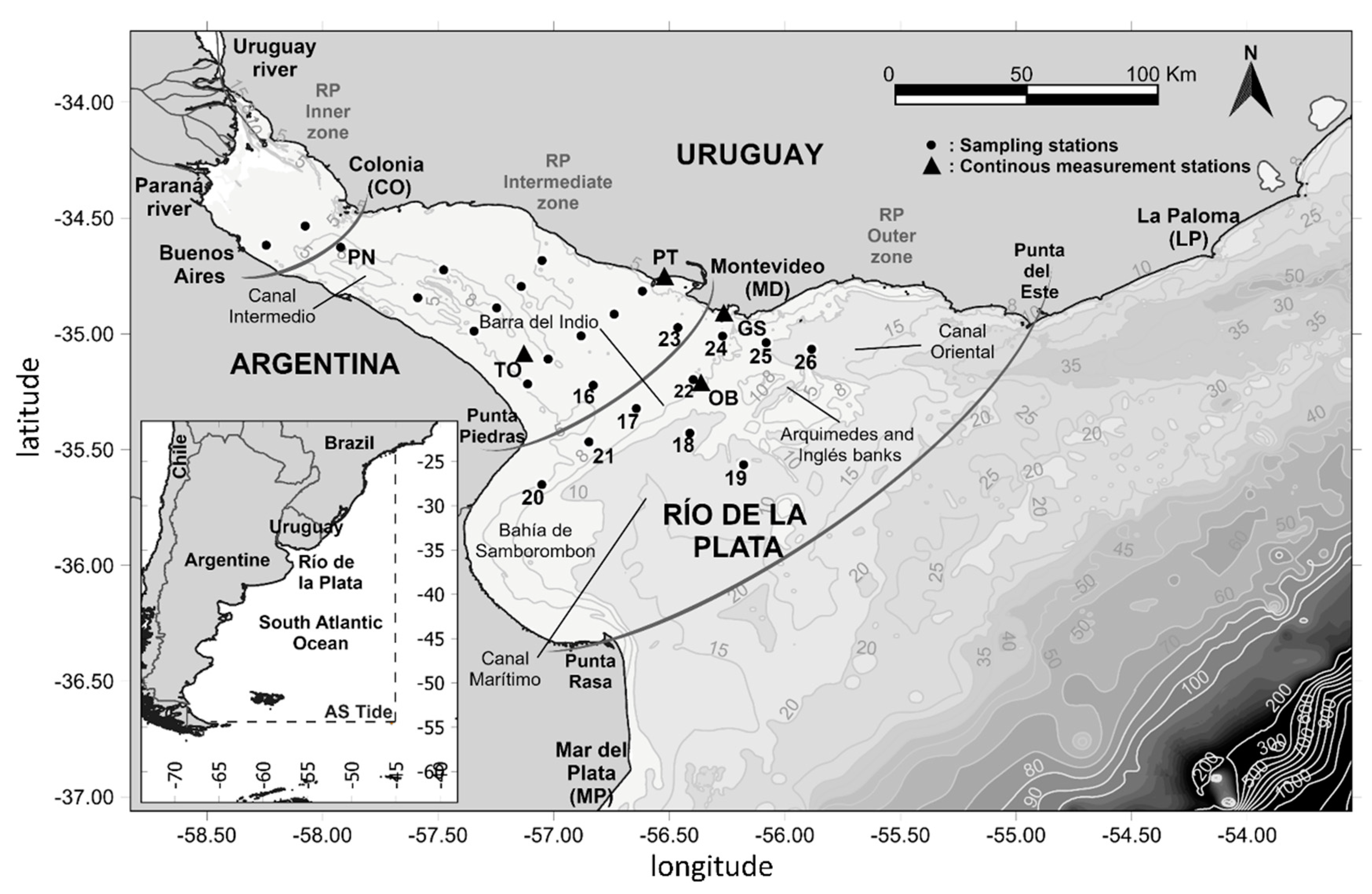
2. The Río de la Plata Estuary

The Río de la Plata, located in South America between Uruguay and Argentina (Figure 1), is a large, wide, and shallow fluvial–estuarine–sea system, classified as microtidal, with a very high fluvial flow, and subtidal oscillations with similar amplitude to the astronomical tidal oscillations (mainly in the northern part). The Río de la Plata extends from the Paraná and Uruguay rivers, discharging into the southwestern Atlantic Ocean. Some relevant dimensions are shown in Figure 1; the inner zone is approximately 2700 km2, the intermediate zone is 9000 km2, and the outer zone is 25,000 km2. The cross-section at the intermediate zone increases from 32 km between Colonia and Buenos Aires to 100 km between Montevideo and Punta Piedras. The cross-section reaches 220 km at the limit of the outer zone between Punta del Este and Punta Rasa. The bathymetry presented in Figure 1 shows depths lower than 10 m in the intermediate zone, with a channel located over the southern coast (‘Canal Intermedio’ channel), while in the outer zone, the ‘Canal Oriental’ channel runs along the northern coast, with depths between 10 and 20 m, as with the ‘Canal Marítimo’ channel on the southern coast; depths greater than 20 m are observed after Punta del Este–Punta Rasa. The continental shelf—with depths greater than 100 m—is located 460 km from the head of the Río de la Plata.
The Río de la Plata receives the fluvial discharge of the Uruguay and Paraná rivers (Figure 1), which is characterised by a mean annual flow of 26,000 m3/s, a 10th percentile of 19,000 m3/s, and a 90th percentile of 32,000 m3/s. The astronomical tide at the Río de la Plata has microtidal characteristics dominated by the semidiurnal M2 signal and K1 and O1 diurnal harmonics. The amplitudes and phases of the main harmonic components at different stations at the Río de la Plata have been presented by Santoro et al. [18] (see Table 2), who showed that the tidal amplitude is greater at the southern coast (the M2 harmonic amplitude is 0.35 m at MP, 0.31 m at TO, and 0.27 m at BA) than at the northern coast (the M2 harmonic amplitude is 0.12 m at LP, 0.14 m at MD, and 0.16 m at CO; see station locations in Figure 1). The non-astronomic tidal component of the sea level variation at the Río de la Plata is very relevant, in terms of both amplitude and frequency [18,24]. Santoro et al. [18] calculated the ratio between the variance of the meteorological tide series and the variance of the observed sea surface elevation series at seven stations in the Río de la Plata; their results showed that, on average, more than 50% of the sea level variability in the study area is related to meteorological tide events.
According to Fossati et al. [24], there is important spatial and temporal variability in the Río de la Plata hydrodynamic and salinity distribution. There is a clear difference between the behaviour observed in the inner/intermediate zones and in the outer zone. In general terms, the salinity front is located inwards at deeper zones (e.g., the ‘Canal Marítimo’ and ‘Canal Oriental’ channels), where saline stratification is more pronounced. Then, the residual velocities in the intermediate zone are fundamentally two-dimensional, typical of river discharge (net transport outwards). On the other hand, the outer zone presents more complex three-dimensional characteristic patterns, with residual velocities in the incoming flow towards the continent in the deeper zones, and discharge flow through the shallower coastal zones. Finally, in the front area, the residual current is almost null. In addition to these spatial differences, the meteorological conditions—particularly, calm versus storm conditions—have a great influence on the dynamics, especially in terms of salinity and fine sediments.
Salinity measurements in the Río de la Plata are scarce. The most extensive measurement campaign was carried out between 2010 and 2011, during the International FREPLATA–IFREMER Project [27]. During this project, continuous salinity measurements were recorded at two locations (OB and TO in Figure 1), using SMATCH equipment fabricated by the NKE instrumentation company. One of the instruments used was at an oceanographic buoy (OB) deployed 30 km south of Montevideo (Lat 35°12′0.00″ S, Long 56°24′0.00″ W), close to the limit between the intermediate and outer zones of the estuary. The mean water depth in the area was 8 m, and the salinity measurements were taken approximately 2.5 m below the water surface. The second location was at an oceanographic tower (Torre Oyarvide, TO in Figure 1), located 18 km from the Argentinian coast (Lat 35°06′0.00″ S, Long 57°07′48.00″ W), in the intermediate zone of the estuary. The mean water depth in the area was 7 m, and the salinity measurements were taken 5 m above the bed. In the OB buoy, a meteorological station was also installed. Additionally, six field campaigns were performed, and several salinity profiles were obtained using CTDs in the region of the salinity front (measured stations 16–25 in Figure 1). The details of the installed instruments, their configuration, and data quality assessments can be found in the work of Simionato et al. [27].

3. Hydrodynamic Numerical Modelling

3.1. Model Description

The 3D model implementation at the Río de la Plata and its maritime front (henceforth denoted as RPtide) was based on the MOHID water surface model [28]. MOHID solves the 3D baroclinic free-surface Reynolds-averaged Navier–Stokes equations with Boussinesq and hydrostatic approximations. MOHID comprises an integrated modelling philosophy, not only involving processes (physical and biogeochemical), but also different scales (allowing for the use of nested models) and systems (estuaries and watersheds). MOHID encompasses a standard finite-volume approach, using a generic combination of sigma and/or Cartesian vertical coordinates with an ADI semi-implicit scheme for the horizontal advection–diffusion numerical schemes, as well as possessing a complete suite of modern and standard open boundary conditions.
The RPtide model is a local high-resolution 3D hydrodynamic baroclinic model with ten vertical sigma layers. The RPtide domain (Figure A1 of the Appendix A) was between the Río de la Plata’s head (i.e., where the rivers discharge) and the area bounded between Mar del Plata (Argentina) and Rio Grande (Brazil), extending approximately 170 km offshore. It is forced, at the oceanic boundary, with water levels and currents from the regional AStide model [29]. The AStide model is a 2D hydrodynamic barotropic implementation of the MOHID numerical model, implemented for the South Atlantic Ocean with a grid of 0.1° resolution in longitude and latitude. It is forced by NCEP reanalysis winds [30] and the FES2004 astronomical tide model [31]. The AStide model has been calibrated and validated using water-level measurements [29].
The RPtide model is forced by the resulting data of hourly sea surface elevation and hourly barotropic currents from the AStide model at oceanic boundaries, by high-resolution winds on the surface obtained from the ECMWF (European Centre for Medium-Range Weather Forecast) global database [32] with a spatial resolution of 0.25° and a temporal resolution of 6 h, and by daily flowrates at the Uruguay and Paraná rivers. The three-dimensional mesh has a latitude–longitude structure, constant horizontal discretisation of 0.02°, and 10 vertical layers, defined from sigma coordinates using a constant coefficient. The RPtide model configuration includes the Coriolis force effect. The Smagorinsky model was used for the calculation of horizontal eddy viscosities. Vertical mixing was modelled in MOHID using the general ocean turbulence model (GOTM) [33]. The bottom stress was computed using a quadratic law formulation with an absolute roughness coefficient. The wind stress at the surface was considered and parameterised by a wind drag coefficient, calculated using the formulation of Large and Ponds [34]. The model time step was 90 s. In this work, an extensive period of 10 years was simulated (2006–2015).
The model was calibrated and validated in previous studies using sea surface levels measured at Pilote Norden, Torre Oyarvide, and Montevideo (PN, TO, and MD, respectively), along with current profiles (ADCP measurements at the OB location) and salinity time series at the oceanography buoy (OB) [22] (see the station locations in Figure 1). The quality of the model results was evaluated using the root-mean-square Error (RMSE), obtaining values of 0.22 m at PN, 0.23 m at TO, and 0.18 m at MD for the sea surface levels. For the current speed, a vertical average of 0.18 m/s of error and, for the salinity, an error of 4 ppt at OB [22] was observed. The details of the calibration process of the model can be found in Appendix A.

3.2. Model Validation

In order to improve the evaluation of the model performance in the salinity dynamic representation, new comparisons between measured data and model results were conducted. The vertical profiles measured during the FREPLATA–IFREMER Project were used to evaluate the quality of the model in the representation of the vertical salinity variations.
Figure 2 presents the salinity profiles at 11 locations, measured during four field campaigns carried out during 2010 (March, June, August, and October), as well as the comparison with model results. The profiles obtained with the numerical model during the days of the measurements are presented hourly, from 12 h before the survey until 12 h after it (i.e., 24 model profiles are shown for each measured profile). The collected salinity profiles showed a wide range of stratification conditions, from vertical mixing to strong stratification conditions. For example, the profiles collected during March 2010 showed a mainly vertical salinity stratification, except for those measured at stations 16, 23, and 24. For the data collected during June 2010, some profiles showed quite uniform conditions (stations 16, 18, 19, 20, and 24), while others showed marked stratification (stations 17, 21, 22, 23, 25, and 26). For the data collected during August 2010, the data showed a strong stratification condition at all measuring stations, while the last campaign during October 2010 showed mostly mixed vertical salinity conditions, with some weak stratification at only some of the measuring stations. These data clearly indicate the great spatial and temporal variability of the vertical salinity distribution in the salinity front area. Comparing measured and simulated instantaneous vertical salinity profiles is very exigent. Figure 2 shows that the model was able to produce both mixed and stratified conditions at most stations. Although the modelled salinity values showed differences from those measured, in most cases, the vertical distribution was reasonably well represented.

3.3. Analysis of Model Results

The spatiotemporal variability of salinity and stratification in the Río de la Plata was analysed based on the numerical results of the RPtide model. The temporal variability was characterised at different temporal scales: annual, monthly, and storm. At the same time, the influence of fluvial flow and winds was determined.
In this paper, stratification is defined as the difference between the salinity at the bottom and that at the surface, while the normalised stratification is defined as the stratification divided by the vertical integrated salinity. Using the numerical model results, the stratification and the normalised stratification were calculated for each instant and node, as follows:
S t r a t i f i c a t i o n ( x , y , t ) = S a l i n i t y ( x , y , z = 10 , t ) S a l i n i t y ( x , y , z = 1 , t ) , N o r m a l i z e d   S t r a t i f i c a t i o n   ( x , y , t ) = S t r a t i f i c a t i o n   ( x , y , t ) / M e a n   S a l i n i t y   ( x , y , t ) , M e a n   S a l i n i t y ( x , y , t ) = 1 d e p t h ( x , y ) z = 1 z = 10 S a l i n i t y ( x , y , z , t ) d z .
The salinity stratification and normalised salinity stratification were calculated from the 10-year (2006–2015) hourly numerical results, for the entire domain. In order to analyse the annual variability and the influence of fluvial flow on the stratification, the yearly averaged salinity stratification and the yearly normalised stratification were calculated and correlated with the annual fluvial flow. Additionally, the monthly scale variability—and the influence of the fluvial flow—was analysed, by selecting one year and calculating the monthly average stratification and normalised stratification.
The spatiotemporal variability at storm scale was analysed by considering the salinity and stratification field before, during, and after storms with different main wind directions. In this study, we use the term storm when the wind intensity (obtained from the ECMWF reanalysis) was over 13 m/s at the OB location (see Figure 1). This condition is observed about 5–10 times a year. The storms of two particular years with fluvial discharges (one year with a relatively low annual mean fluvial flow, and another year with a relatively high annual mean fluvial flow) were analysed, in order to identify the existence of common flow and stratification patterns.

4. Results

4.1. Fluvial Flow Influence

Considering the period between 2006 and 2015, the annual mean fluvial flow from the combined Uruguay and Paraná rivers showed high variability, ranging from 16,000 m3/s (in 2006) to 36,000 m3/s (in 2015) (Figure 3). The spatial variation of the annual mean stratification calculated with the numerical model for this period is presented in Figure 3; in order to analyse its tendency, the results are ordered according to increasing annual mean flow. The results indicate that the highest stratification was observed in the deeper zones of the external Río de la Plata (Canal Oriental and Canal Marítimo). The shallow areas of this zone—the Arquimedes and Inglés banks and Bahia de Samborombón—presented low mean stratification values.
Analysing the correlation between the annual stratification and the tributary mean flow, there was a tendency of higher stratification and more extensive area of stratification with higher annual mean flows. For the years with lower annual mean flow (2006, 2008, 2009, and 2012), the results showed that an area close to Montevideo experienced up to 10 ppt of stratification. With higher annual flow (2017, 2013, 2010, and 2011), this area extended towards the east. In these conditions, the stratification increased over the Canal Marítimo channel zone at the central Río de la Plata, and extended towards the ocean. Finally, with the highest annual flows (2014 and 2015), the stratification reached values greater than 12 ppt and covered all of the external Río de la Plata zone, except for the shallow areas of Bahia de Samborombón, the Uruguayan coast, and the Arquimedes and Inglés banks. The same tendency was observed in the normalised stratification fields (Figure 4). This means that both the average salinity stratification and the normalised stratification increased in magnitude and extent with an increase in the fluvial flow of the Paraná and Uruguay rivers, in terms of the annual variability scale.
In Figure 5, the annually averaged salinity fields at the bottom and surface for the years with the highest, middle, and lowest annual mean river flow (2006, 2007, and 2015, respectively) are presented. Focusing on the bottom fields, the 2006 and 2007 are very similar, with the isohaline of 30 ppt being situated around the exterior limit of the Río de la Plata, while for 2015 there were values of 25 ppt around the same limit. When we focus on the surface fields, the differences between the three years were more noticeable, which is clearly reflected in the isohalines in Bahia de Samborombón, or along the Uruguayan coast between Montevideo and Punta del Este, generating variation in the stratification fields. The results clearly show that high annual average fluvial flow generates the extent of the freshwater area, with a higher longitudinal salinity gradient and the change in the location of the salinity front towards the ocean.
In order to study the influence of the fluvial flow on the monthly variability of the salinity stratification, the correlation between the monthly averages of the variables was analysed. The year 2014 was selected, due to its large monthly average fluvial flow variability, from values of 22,400 m3/s (January) to 48,900 m3/s (July) (Figure 6). The mean salinity stratification obtained with the numerical model for each month of the year, ordered according to increasing fluvial flow, is presented in Figure 6. The tendency at the monthly scale was not as clear as that observed at the annual scale. The monthly average stratification fields showed high spatial variability and extent; for example, the stratification fields obtained for February and April (or December and July) were quite similar, but the fluvial flow varied a lot. Nevertheless, by analysing the monthly normalised salinity stratification fields, a correlation with the monthly mean river flow was again obtained. The results presented in Figure 6 clearly show the increase in the normalised stratification values and the increase in the extent of the stratified area as the monthly fluvial flow increased. It seems that the computation of the normalised stratification filtered out events such as storms, which may generate instantaneous changes in the distribution of the bottom and surface salinities.

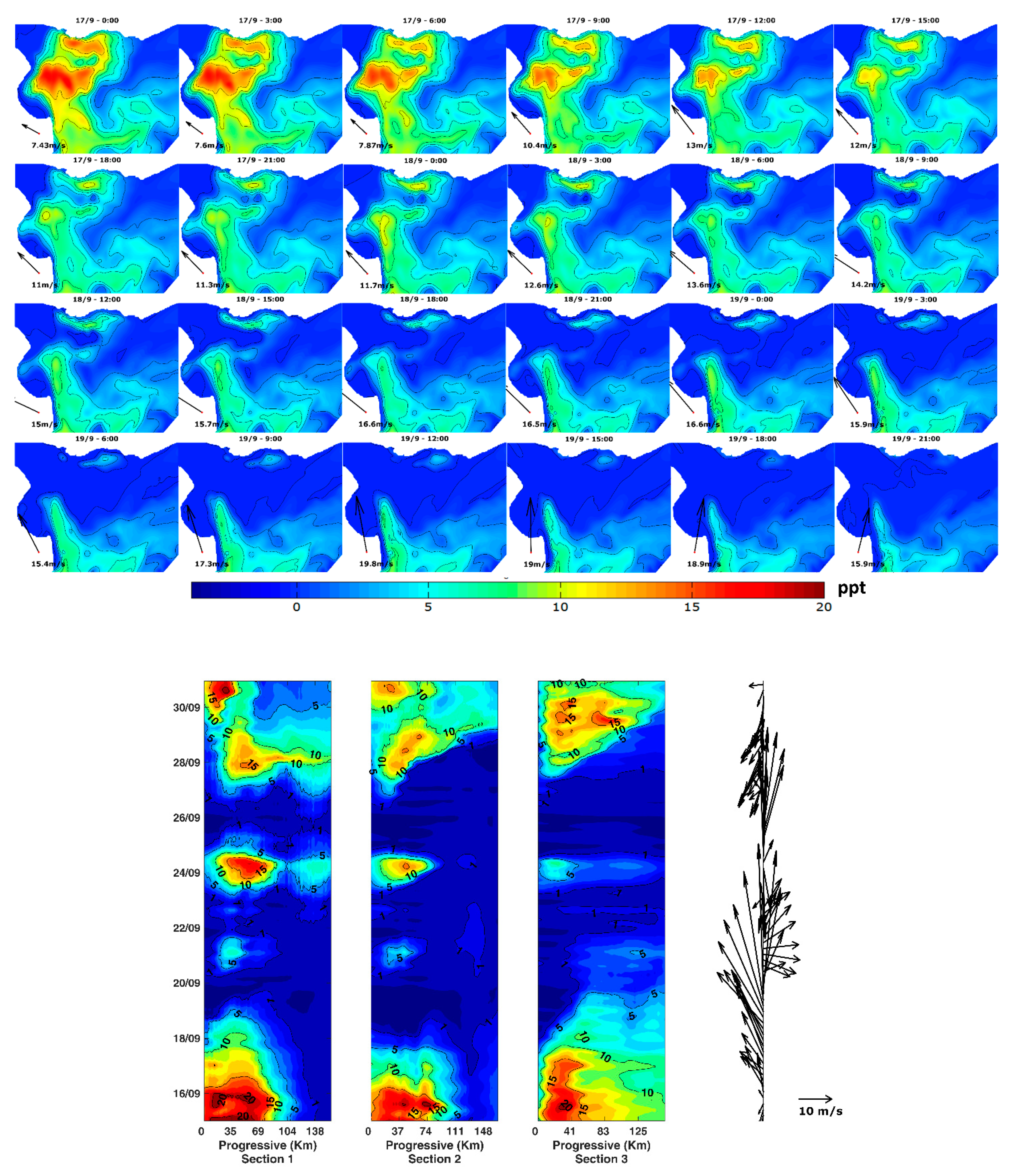
4.2. Influence of Storms

The analysis of the salinity variability during storms was based on the numerical results for the years 2012 and 2014—one year with low annual mean flow and another with high annual mean flow, respectively. These years were selected in order to represent a wide range of fluvial flow conditions. In Table 1, the storms that were analysed in this study are summarised, indicating their date (month) of occurrence, maximum intensity, main wind direction, and duration. The effects of the storms were studied by analysing the spatial variability in the domain and along three longitudinal sections before, during, and after the duration of the storm. The longitudinal sections presented in Figure 7 were defined to cover the deeper northern zone (Canal Oriental), the deeper southern zone (Canal Marítimo), and the shallow middle zone (Arquimedes and Inglés Banks).
Figure 8 shows an example of the temporal evolution of the stratification (3-h time steps) for a storm with a main wind direction from the southwest (April 2014). Figure 8 also presents the results (in a Hovmoller diagram) of the stratification for the longitudinal sections (Figure 7). The effects of other identified storms coming from the southwest were quite similar. Before the storm, there was a marked stratification at the outer Río de la Plata zone, with high values mainly at the deeper channels. This can be seen clearly in the Hovmoller diagram, where the highest stratification values in the deeper section are noted (Section 1). As the wind increases, it is observed that the stratification starts to vanish due to the mixing process (between 13 and 15 April). Consequently, a total mixing (very low stratification) is observed, which was maintained up to two days after the peak of the storm. After that, the stratification was observed to gradually redevelop, mainly over the zone of the salinity front and along the Uruguayan coast.
Complementing the stratification analysis for the southwest storm, the bottom and surface salinity fields before the storm, a few hours after the peak of the storm, and two days after the storm are presented in Figure 9. Due to the storm, the bottom salinity field changed from a stable field that followed the bathymetry to a field corresponding to a water discharge along the northern coast. No significant changes were observed in the central zone or at the Bahia de Samborombón and, after the storm, the bottom salinity field returned to its previous condition. The effect of the southwest storm on the surface salinity field was the same as for the bottom salinity (i.e., the generation of a discharge along the north coast). Before the storm, the surface salinity showed the freshwater extending along the Uruguayan coast, along the central zone (Canal Marítimo channel), and along the Bahia de Samborombón. During the storm, the discharge along the Uruguayan coast was enhanced, and the freshwater plume along the south coast disappeared. In these conditions, the salinity front rotated and established between Punta Piedras and Punta del Este; furthermore, the surface salinity field became almost equal to the bottom salinity field.
The effect of a storm coming from the northwest was quite similar, in terms of the southern and central parts of the Río de la Plata, to that of the storms coming from the southwest, and the mixing increase and the stratification decrease were related to the intensity of the storm. Nevertheless, the stratification kept to the northern coast. An example is presented in Figure 10 where, for a northwest storm, the stratification field every 3 h for the storm in July 2014 is shown. The Hovmoller diagram of the stratification during the storm in the three sections is also presented in Figure 10. The results show that the storm generated mixing in the southern and central parts of the Río de la Plata, shown clearly in longitudinal Section 2 and Section 3 between 7 and 8 July, while stratification was maintained at the northern coast (Section 1). Generally, northwest storms have shorter duration than southwest storms and, thus, their effect on vertical mixing is less predominant.
Figure 11 shows the temporal variation (every 3 h) and the Hovmoller diagram of the stratification during a storm coming from the southeast with a maximum intensity of 19 m/s, which took place in September 2012. Before the storm, most of the study area was stratified. When the storm started, the stratification decreased from west to east, reaching a state of mixing in the whole area. Therefore, the effect of a southeast storm is clearly an increase in the mixing process. From the Hovmoller diagram, it can be observed that, after the storm, the stratification took a few days to redevelop.
Finally, the response of the stratification field to a storm coming from the northeast is presented in Figure 12, where the stratification every 3 h and the Hovmoller diagram in the longitudinal sections during the storm that took place in June 2014 are shown. Before the storm, there was stratification in most parts of the external zone of the Río de la Plata. When the intensity of winds increased, the stratification also increased; furthermore, it extended towards the south and towards the ocean. After the storm, the stratified area was more extended towards the ocean, compared to the previous condition. The common pattern of northeast storms is an increase in the stratified area.

5. Discussion

Continuous measurements in several vertical positions, in order to analyse the temporal evolution of the vertical salinity profile in the Río de la Plata, are not available. Nevertheless, by analysing several CTD vertical salinity profiles obtained from 11 stations during four campaigns distributed in the salinity front area of the Río de la Plata, it was possible to determine some characteristics of the vertical variability. The stations located in the northern zone (stations 23, 24, 25, and 26; in the Canal Oriental) showed vertical salinity stratification in three of the four campaigns. The stations located on a transect between Canal Marítimo and Arquimedes Bank (stations 16, 17, 18, and 19) indicated basic stratification in two campaigns and mixing conditions in the other two. The other stations (20, 21, and 22) showed quite similar behaviour, with both conditions. Considering the classification of estuaries based on the vertical salinity structure, the analysed salinity profiles showed a wide range of vertical mixing and stratification conditions, changing from well-mixed conditions to weakly and strongly stratified ones.
The results presented in this paper complement those described by Fossati et al. [24], who presented salinity time series measured at TO and OB (see locations in Figure 1). According to Fossati et al. [24], the data collected at TO suggest that the salinity front rarely reaches the TO station, except when the Río de la Plata is hit by significant storms. In such occurrences, the measurements show a sharp salinity increase and high water level values, associated with the meteorological storm surge during the storm. The salinity time series measured at OB showed a high temporal variation, with salinity values between 0 and 20 ppt. According to Fossati et al. [24], the salinity measured at OB also increased as a consequence of offshore water being pushed towards the estuary by strong southerly winds.
Complementing the salinity data, the use of numerical models is essential to study the hydrodynamic and salinity variability of estuaries, including the Río de la Plata. In this study, we used a 3D hydrodynamic model (RPtide), which has been continually improved by our research group [20,22,29,35]. Originally, validation of the salinity results was only possible using the salinity time series registered at OB and TO [22]. In this study, the model was validated using vertical profiles collected during four surveys at different locations of the salinity front. Although the exact measured profile values were not reproduced by the model, the difference in the stratified conditions related to calm-weather and storm conditions, as observed in the measurements, were well reproduced by the model; this indicates that the vertical diffusion processes were reasonably represented in the numerical model, as were the wind stress processes.
Although the numerical model has limitations, it is capable of representing the main characteristics of the spatiotemporal variability of salinity in the estuary, and allows for extension of the analysis to the whole Río de la Plata and maritime front, under a wide range of weather and forcing conditions. From hourly salinity results of a long simulation period of 10 years (2006–2015), several results were obtained relating to the stratification and salinity variability at the Río de la Plata. The influence of the fluvial flow of the Paraná and Uruguay rivers over the salinity variability was studied, using the annual mean values, in order to filter the effects of tides and storms. From 2006 to 2015, the annual mean fluvial flow varied from 16,000 m3/s (in 2006) to 36,000 m3/s (in 2015). The results show that the higher the mean fluvial flow, the more extended and intense the obtained stratification. The mean salinity at the bottom is not as dependent on the mean fluvial flow, but the mean surface salinity showed much higher differences between years, generating the variability in the stratification. The results show very clearly that high annual average fluvial flows generate an extension of the freshwater area, with larger longitudinal salinity gradients and a change in the location of the salinity front towards the ocean. As the fluvial discharge increases, the surface layer of freshwater increases in extent and, therefore, there is an inflow of salinity through the bottom layer; This has two consequences: the increment of magnitude, and the extension of mean salinity stratification and normalised stratification. These results are similar to those presented by Maciel et al. [36], who analysed the influence of the fluvial flow over the turbidity front in the Río de la Plata.
Due to the large variation in the monthly mean fluvial flow (e.g., from 22,400 m3/s to 48,900 m3/s in the year 2012), we analysed its effect on the normalised salinity stratification (i.e., the ratio between the salinity stratification and the mean vertical salinity) on a monthly scale. While the monthly average stratification fields did not show a clear correlation with the monthly mean river flow, the monthly normalised salinity stratification fields showed a clear correlation with it. Compared to the classic stratification parameter, it seems that the normalised stratification filters out relevant events, such as storms, at a monthly temporal scale.
In relation to the effects of storms on the salinity field variability, the numerical model results showed a high influence, depending on the duration, intensity, and wind direction of the storm. The effect of a storm coming from the northwest is quite similar to that of storms coming from southwest, especially in the central and southern zones of the Río de la Plata: the mixing increases, and the stratification decreases, according to the intensity of the storm. By analysing the salinity field, it was observed that strong storms from the west generated a flow over the Uruguayan coast towards the ocean, moving the surface salinity field in concordance with the mean bottom salinity field. However, strong winds coming from the east and northeast generate a salty inward flow for the Uruguayan coast, and a less salty outflow for the Canal Marítimo channel, which is opposite to the more stable bottom salinity field. The effect of south–southeast storms was also to increase the mixing process and reduce stratification. Interestingly, the opposite effect was identified for northeast storms, where an increase in the stratified area was observed. Analysis of the salinity response to storms showed that neither the mixing process generated for the storms coming from the west or southeast, nor the stratification generated for the northeast storms, were conditioned by the mean fluvial flow.
Unlike the results obtained by Simionato et al. [14] and Meccia et al., [19], which associated the vertical mixing of salinity only with strong southeasterly winds, our results showed that mixing processes occur for storms coming from the northwest–west and southwest–south–southeast. Although the study presented by Meccia et al. [19] was also based on a numerical modelling approach, the main differences in the results were probably because their model was forced at the oceanic boundary only by the M2 tidal constituent, thus ignoring the meteorological tide effect.
Finally, based on the model results, it was possible to construct a spatiotemporal characterisation of the vertical stratification conditions over the whole estuary. Figure 13 presents the frequency associated with vertical salinity stratification higher than 5 ppt for the 10 simulated years (2005–2015). Although this was an arbitrary limit value, it separated two clearly different conditions of the vertical salinity structure identified in the Río de la Plata: stratified, and well-mixed. It can be seen that the higher frequencies (80%) were obtained on the northern coast (Canal Oriental). The stratification frequency was close to 70% in the Canal Marítimo, while it was around 60% in the outer zone of the estuary. Both the Arquimedes and Ingles Banks and the Bahia de Samborombón presented low stratification frequency. Related to the classical estuarine vertical structure classification presented by Valle-Levinson [2], it was possible to confirm that, in an average classification, the Río de la Plata presents strongly stratified conditions in the deeper zones (Canal Marítimo and Canal Oriental), well-mixed conditions in the shallow areas (Arquimedes Bank and Samborombón Bay), and weakly stratified conditions (or partially mixed, according to Dean, [6]) in the rest of the Río de la Plata, inward to the fluvial discharge zones and outward to the Atlantic Ocean.

6. Conclusions

From numerical modelling results and recent in situ measurements, the main aspects of the spatiotemporal variability of the salinity and vertical salinity stratification in the Río de la Plata were studied. Complementing salinity data with numerical modelling is essential in the study of the temporal and spatial variability of large estuaries, such as the Río de la Plata. Measured vertical salinity profiles distributed in the front area of the Río de la Plata showed a wide range of vertical mixing and stratification conditions, changing from well-mixed to weakly and strongly stratified conditions. The numerical model was able to reproduce the different stratification conditions related to calm weather and storm events.
The numerical model allowed us to extend the analysis to the whole Río de la Plata and maritime front, under a wide range of weather and forcing conditions. Regarding the influence of the fluvial flow of the Paraná and Uruguay rivers on the salinity dynamics, the results showed that the higher the mean fluvial flow, the more extended and stronger the obtained stratification. The mean salinity at the bottom showed less variability with respect to the mean fluvial flow than the mean surface salinity, thus generating variability in the stratification. The results clearly show that high annual average fluvial flows increase the extent of the freshwater area, with larger longitudinal salinity gradients, and change the location of the salinity front towards the ocean.
Regarding the effect of storms on the salinity field, the numerical modelling results showed a high influence, depending on the duration, intensity, and wind direction of the storm. The effect of a storm coming from the northwest was quite similar to that of storms coming from the southwest, especially in the central and southern zones of the Río de la Plata, both generating increased mixing and decreased stratification, according to the intensity of the storm. The effect of south–southeast storms is also to increase the mixing process and reduce stratification. Strong storms from the west generate a flow over the Uruguayan coast towards the ocean, moving the surface salinity field in concordance with the mean salinity bottom field. Interestingly, strong winds coming from the east and northeast generate a salty inward flow along the Uruguayan coast, and a less salty outflow for the Canal Marítimo channel, which is opposite to the more stable bottom salinity field, thus increasing the stratified area. Neither the mixing process generated for the storms coming from the west or southeast, nor the stratification generated for the northeast storms, were conditioned by the mean fluvial flow.
Although the numerical model used herein represents the main characteristics of the salinity behaviour in the estuary, it has limitations. Further steps include improving the representation of the temporal variability and horizontal extension of the salinity front, increasing the numerical model spatial resolution, and recalibrating the wind stress.

Author Contributions

Conceptualization, M.J. and M.F.; methodology, M.J. and M.F.; formal analysis, M.J. and G.S.; investigation, M.J. and M.F.; writing—original draft preparation, M.J., P.S. and M.F.; writing—review and editing, M.J., G.S., P.S. and M.F.; supervision, M.F.; project administration, M.F.; funding acquisition, M.F. All authors have read and agreed to the published version of the manuscript.

Funding

This research received no external funding.

Institutional Review Board Statement

Not applicable.

Informed Consent Statement

Not applicable.

Data Availability Statement

Not applicable.

Conflicts of Interest

The authors declare no conflict of interest.

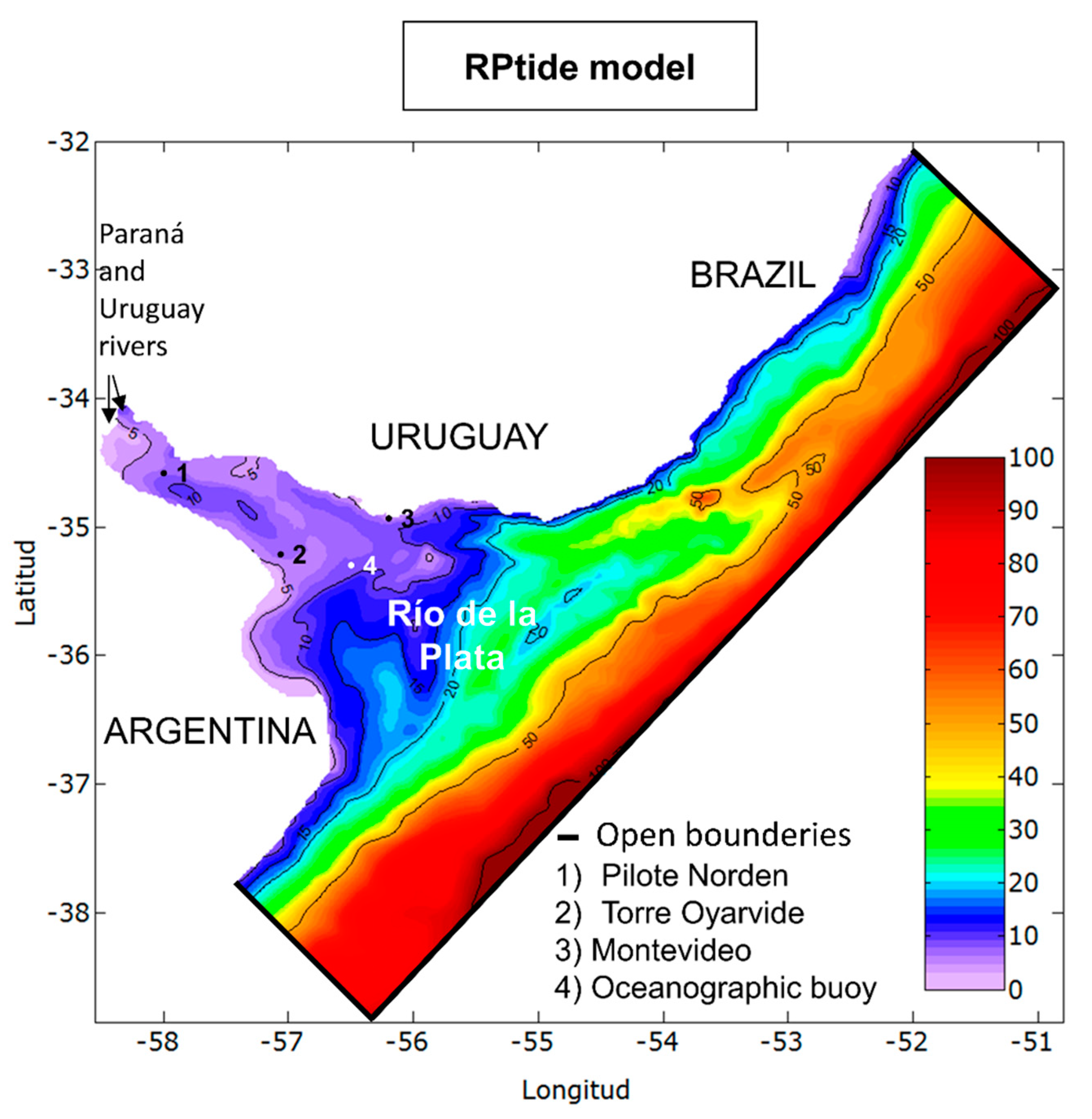
Appendix A. RPtide Model Implementation and Calibration

The RPtide model is an implementation of the 3D hydrodynamic baroclinic model MOHID, based on the implementation of a previous model described by Fossati et al. [20]. The main improvement, with respect to the previous MOHID implementation for the Río de la Plata, was related to the main forces and the associated boundary conditions.
The RPtide domain is presented in Figure A1. The RPtide model implementation is characterised by the following:
(1)
Latitude–longitude coordinate system;
(2)
Horizontal grid with constant resolution of 0.02° × 0.02°;
(3)
Vertical grid with 10 uniformly distributed sigma layers;
(4)
Bathymetry from charts published by the Uruguayan Oceanographic, Hydrographic, and Meteorological Service of the Army (SOHMA) and the Argentinian Naval Hydrographic Service (SHN);
(5)
Coastline from the NOAA/NGDC Marine Geology and Geophysics Division database and from local high-resolution measurements;
(6)
Bottom stress is computed using a quadratic law formulation with a roughness length;
(7)
Free-surface boundary conditions: winds and pressure from global reanalysis of ECMWF (European Centre for Medium-Range Weather Forecast) data, with a spatial resolution of 0.25° and temporal resolution of 6 h;
(8)
Oceanic boundary conditions: astronomical and meteorological tides (water level and 2D currents) from the barotropic 2D hydrodynamic model of the South Atlantic Ocean (AStide) in each cell of the southwest and northeast boundaries and every two cells in the southeast boundary;
(9)
Continental boundary condition: daily mean values of the fluvial discharges of the Uruguay and Paraná (two branches: Paraná-Guazú and Paraná-Las Palmas) rivers;
(10)
Time step of 90 s;
(11)
The vertical viscosity is solved by the GOTM model;
(12)
The horizontal viscosity is solved by the Smagorinsky model, with a coefficient of 0.1;
(13)
The diffusivity (horizontal and vertical) is related with viscosity through the Schmidt number;
(14)
The wind stress at the surface is applied and parameterised by a wind drag coefficient, calculated using the formulation of Large and Ponds;
(15)
For the salinity, the boundary conditions are freshwater for the continental boundary and a fixed value of 35 ppt for the oceanic boundary;
(16)
Initial conditions: zero velocity, constant water level, and uniform salinity;
(17)
Spin-up period: a long period (1 year) is required for the initial salinity condition.
The calibration test and range parameters are presented in Table A1; the calibration period was July 2010. The results were evaluated using sea level measurements at PN and TO, as well as salinity time series measured at OB (see measured stations location in Figure A1). Table A2 presents the RMSE obtained for each variable in the calibration test, while Figure A2 shows a time-series comparison. The selected configuration is the one named Final. The validation period corresponds to the years 2009 and 2010; the results were evaluated using sea level measurements at PN, TO, and MVD, current profiles (ADCP measurements) at OB, and salinity time series measured at OB. Table A3 shows the RMSE values obtained for the validation period for water levels, velocity, and salinity. The quality of the model results was even better during the validation stage. The validation results are presented in Alonso et al. [22] (Figure 6, Figure 7 and Figure 8).
Figure A1. RPtide model domain, bathymetry (m), and location of stations.
Jmse 09 00860 g0a1
Table A1. RPtide model calibration test and range parameters. Ref is the reference simulation; for the other simulations, only the modified parameters are shown. The parameters for the selected configuration after the calibration process are referred to as Final.
Simulation NameRugosityNº SchmidtOceanic BCObjective
Ref0.000650.2Blumber and Kanta Radiation condition Tlag = 1000 sReference simulation
Sim10.001--Rugosity influence
Sim20.0001--Rugosity influence
Sim3-0.1-Nº Sch influence
Sim4-0.5-Nº Sch influence
Sim5-1-Nº Sch influence
Sim6--Flather conditionOceanic BC influence
Sim7--Blumber and Kanta Radiation condition Tlag = 5000 sOceanic BC influence
Final0.0010.2Blumber and Kanta Radiation condition Tlag = 1000 sSelected configuration
Table A2. Statistics for the calibration period (July 2010), for water levels at PN and TO and salinity at BO.
Simulation NameRMSE (m) Water Level PNRMSE (m) Water Level TORMSE (ppt) Salinity BO
Ref0.340.243.39
Sim10.330.243.38
Sim20.350.253.39
Sim30.340253.72
Sim40.330.243.23
Sim50.330.233.55
Sim60.350.323.15
Sim70.360.243.03
Final0.320.233.45
Figure A2. RPtide model calibration test results for the water level (m) at PN (upper panel), for the water level (m) ar TO (middle panel), and for salinity (ppt) at BO, with respect to data obtained in July 2010.
Jmse 09 00860 g0a2
Table A3. Statistics obtained during the validation stage for water levels at PN, TO, and MVD; velocity currents at BO; and salinity at BO. The periods of time used for the comparison between data and model are provided.
Water Level1 November 2009–31 December 20108 April 2010–25 June 201026 June 2010–31 July 2010
RMSE (m) PN0.240.200.23
RMSE (m) TO 0.230.23
RMSE (m) MVD0.18--
Velocity26 January 2009–18 March 2010--
RMSE (m/s) velocity U BO0.17--
RMSE (m/s) velocity V BO0.18--
Salinity26 November 2009–22 January 2010-25 June 2010–31 July 2010
RMSE (ppt) BO4.57-3.65

References

  1. Prandle, D. Estuaries: Dynamics, Mixing, Sedimentation and Morphology; Cambridge University Press: Cambridge, UK, 2009. [Google Scholar] [CrossRef]
  2. Valle-Levinson, A. (Ed.) Contemporary Issues in Estuarine Physics; Cambridge University Press: Cambridge, UK, 2010. [Google Scholar] [CrossRef]
  3. Valle-Levinson, A. Large Estuaries (Effects of Rotation). In Treatise on Estuarine and Coastal Science; Wolanski, E., McLusky, D., Eds.; Academic Press: Cambridge, MA, USA, 2011; pp. 123–140. ISBN 9780080878850. [Google Scholar]
  4. Pritchard, D.W. Estuarine circulation patterns. Proc. Am. Soc. Civ. Eng. 1955, 81, 1–11. [Google Scholar]
  5. Cameron, W.M.; Pritchard, D.W. Estuaries. In The Sea; Hill, M.N., Ed.; John Wiley & Sons: New York, NY, USA, 1963; Volume 2, pp. 306–324. [Google Scholar]
  6. Dyer, K.R. Estuaries. In A Physical Introduction; John Wiley & Sons: New York, NY, USA, 1997. [Google Scholar]
  7. Davies, J.H. A morphpgenetic approach to world shorelines. Z. Geomorphol. 1964, 8, 127–142. [Google Scholar] [CrossRef]
  8. O’Callaghan, J.; Pattiaratchi, C.; Hamilton, D. The response of circulation and salinity in a micro-tidal estuary to sub-tidal oscillations in coastal sea surface elevation. Cont. Shelf Res. 2007, 27, 1947–1965. [Google Scholar] [CrossRef]
  9. Geyer, W.R. Influence of Wind on Dynamics and Flushing of Shallow Estuaries. Estuar. Coast. Shelf Sci. 1997, 44, 713–722. [Google Scholar] [CrossRef]
  10. Huang, W.; Li, C.; White, J.R.; Bargu, S.; Milan, B.; Bentley, S. Numerical Experiments on variation of freshwater plume from Mississippi River diversion in Lake Pontchartrain estuary. J. Geophys. Res Ocean. 2020, 125, C2019JC015282. [Google Scholar] [CrossRef]
  11. Guerrero, R.A.; Acha, E.M.; Framiñan, M.B.; Lasta, C. Physical Oceanography of the Río de la Plata Estuary. Cont. Shelf Res. 1997, 17, 727–742. [Google Scholar] [CrossRef]
  12. Framiñan, M.B.; Valle-Levinson, A.; Sepúlveda, H.H.; Brown, O.B. Tidal variations of flow convergence, shear, and stratification at the Rio de la Plata estuary turbidity front. J. Geophys. Res. 2008, 113, C08035. [Google Scholar] [CrossRef] [Green Version]
  13. Sepúlveda, H.; Valle-Levinson, A.; Framiñan, M. Observations of subtidal and tidal flow in the Río de la Plata Estuary. Cont. Shelf Res. 2003, 24, 509–525. [Google Scholar] [CrossRef]
  14. Simionato, G.C.; Meccia, V.L.; Guerrero, R.; Dragani, W.C.; Nuñez, M. Rio de la Plata estuary response to wind variability in synoptic to intraseasonal scales: 2. Currents’ vertical structure and its implications for the salt wedge structure. J. Geophys. Res. 2007, 112, C07005. [Google Scholar] [CrossRef] [Green Version]
  15. Simionato, C.; Dragani, W.; Meccia, V.; Núñez, M. A numerical study of the barotropic circulation of the Río de la Plata estuary: Sensitivity to bathymetry, the Earth’s rotation and low frequency wind variability. Estuar. Coast. Shelf Sci. 2004, 61, 261–273. [Google Scholar] [CrossRef]
  16. Palma, E.; Matano, R.; Piola, A. A numerical study of the Southwestern Atlantic Shelf circulation: Barotropic response to tidal and wind forcing. J. Geophys. Res. 2004, 109, C08014. [Google Scholar] [CrossRef]
  17. Fossati, M.; Piedra-Cueva, I. Numerical modelling of residual flow and salinity in the Río de la Plata. Appl. Math. Model. 2008, 32, 1066–1086. [Google Scholar] [CrossRef]
  18. Santoro, P.; Fossati, M.; Piedra-Cueva, I. Study of the meteorological tide in the Río de la Plata. Cont. Shelf Res. 2013, 60, 51–63. [Google Scholar] [CrossRef]
  19. Meccia, V.L.; Simionato, C.G.; Guerrero, R.A. The Rio de la Plata estuary response to wind variability in synoptic timescale: Salinity fields and salt wedge structure. J. Coast. Res. 2013, 29, 61–77. [Google Scholar] [CrossRef]
  20. Fossati, M.; Piedra-Cueva, I. A 3D hydrodynamic numerical model of the Río de la Plata and Montevideo’s coastal zone. Appl. Math Modell. 2013, 37, 1310–1332. [Google Scholar] [CrossRef]
  21. Silva, C.; Marti, C.; Imberger, J. Horizontal transport, mixing and retention in a large, shallow estuary: Río de la Plata. Environ. Fluid Mech. 2014, 14, 1173–1197. [Google Scholar] [CrossRef]
  22. Alonso, R.; Jackson, M.; Santoro, P.; Fossati, M.; Solari, S. Wave and tidal energy resource assessment in Uruguayan shelf seas. Renew. Energy 2017, 114A, 18–31. [Google Scholar] [CrossRef]
  23. Fossati, M.; Cayocca, F.; Piedra-Cueva, I. Fine sediment dynamics in the Río de la Plata. Adv. Geosci. 2014, 39, 75–80. [Google Scholar] [CrossRef] [Green Version]
  24. Fossati, M.; Santoro, P.; Mosquera, R.; Martínez, C.; Ghiardo, F.; Ezzatti, P.; Pedocchi, F.; Piedra-Cueva, I. Dinámica de flujo, del campo salino y de los sedimentos finos en el Río de la Plata. RIBAGUA Rev. Iberoam. Del Agua 2014, 1, 48–63. [Google Scholar]
  25. Santoro, P.; Fossati, M.; Tassi, T.; Huybrechts, N.; Pham Van Bang, D.; Piedra-Cueva, I. A coupled wave–current–sediment transport model for an estuarine system: Application to the Río de la Plata and Montevideo Bay. Appl. Math. Model. 2017, 52, 107–130. [Google Scholar] [CrossRef]
  26. Moreira, D.; Simionato, C.G. Modeling the suspended sediment transport in a very wide, shallow, and microtidal estuary, the Río de la Plata, Argentina. J. Adv. Modeling Earth Syst. 2019, 11, 3284–3304. [Google Scholar] [CrossRef]
  27. Simionato, C.; Moreira, D.; Piedra Cueva, I.; Fossati, M. Proyecto FREPLATA—FFEM Modelado numérico y mediciones insitu y remotas de las transferencias de sedimentos finos a través del Río de la Plata. Parte A: Adquisición de datos. Frente Marítimo 2011, 22, 265–304. [Google Scholar]
  28. Mateus, M.; Neves, R. (Eds.) Ocean Modelling for Coastal Management—Case Studies with Mohid; IST Press: Lisbon, Potrugal, 2013. [Google Scholar]
  29. Martínez, C.; Silva, J.P.; Dufrechou, E.; Santoro, P.; Fossati, M.; Ezzati, P.; Piedra-Cueva, I. Towards a 3D Hydrodynamic numerical modeling system for long term simulations of the Río de la Plata dynamic. In Proceedings of the E-Proceedings of the 36th IAHR World Congress, The Hague, The Netherlands, 28 June–3 July 2015. [Google Scholar]
  30. Saha, S.; Moorthi, S.; Pan, H.L.; Wu, X.; Wang, J.; Nadiga, S.; Tripp, P.; Kistler, R.; Woollen, J.; Behringer, D.; et al. The NCEP Climate Forecast System Reanalysis. Bull. Am. Meteorol. Soc. 2010, 91, 1015–1057. [Google Scholar] [CrossRef]
  31. Lyard, F.; Lefevre, F.; Letellier, T.; Francis, O. Modelling the global ocean tides: Modern insights from FES2004. Ocean. Dyn. 2006, 56, 394–415. [Google Scholar] [CrossRef]
  32. Dee, D.P.; Uppala, S.M.; Simmons, A.J.; Berrisford, P.; Poli, P.; Kobayashi, S.; Andrae, U.; Balmaseda, M.A.; Balsamo, G.; Bau-er, D.P.; et al. The ERA-Interim reanalysis: Configuration and performance of the data assimilation system. Q. J. R. Meteorol. Soc. 2011, 137, 553–597. [Google Scholar] [CrossRef]
  33. Villareal, M.; Karsten, B.; Burchard, H.; Demirov, E. Coupling of the GOTM turbulence module to some three dimensional ocean models. In Marine Turbulence. Theories, Observations, and Models; Cambridge University Press: Cambridge, UK, 2005; pp. 225–237. [Google Scholar]
  34. Large, W.G.; Pond, S. Open ocean momentum flux measurements in moderate to strong winds. J. Phys. Ocean. 1981, 11, 324–481. [Google Scholar] [CrossRef] [Green Version]
  35. Santoro, P.; Fernandez, M.; Fossati, M.; Cazes, G.; Terra, R.; Piedra-Cueva, I. Pre-operational forecasting of sea level height for the Río de la Plata. Appl. Math. Modell. 2011, 35, 2462–2478. [Google Scholar] [CrossRef]
  36. Maciel, F.; Santoro, P.; Pedocchi, F. Spatio-temporal dynamics of the Río de la Plata turbidity front; combining remote sensing with in-situ measurements and numerical modeling. Cont. Shelf Res. 2021, 213, 104301. [Google Scholar] [CrossRef]
Figure 1. Río de la Plata: location and bathymetry (in m), as well as main geographical and morphological references. CTD vertical profile stations (numbered dots 16–25) and continuous salinity measurement deployment stations (triangles TO and OB), collected from during the FREEPLATA–FEEM project, are shown.
Jmse 09 00860 g001
Figure 2. Vertical salinity profiles (stations 16–26) measured during the IFREMER surveys in March, June, August, and October 2010, as well as vertical salinity profiles obtained hourly with the RPtide model for each survey at each station from 12 h prior to 12 h after the measured time.
Jmse 09 00860 g002aJmse 09 00860 g002b
Figure 3. Annual average salinity stratification (ppt) obtained with the model for the period 2006–2015, ordered according to increasing annual mean river flow (right corner panel). All maps are in geographic coordinates between Lat (−36.9, −34.7) and Long (−57.4, 54.2).
Jmse 09 00860 g003
Figure 4. Annual normalised salinity stratification for the period 2006–2015, ordered according to increasing annual mean river flow. All maps are in geographic coordinates between Lat (−36.9, −34.7) and Long (−57.4, 54.2).
Jmse 09 00860 g004
Figure 5. Bottom and surface salinity: annual (ppt) average for the years with lower annual mean fluvial flow (2006), middle annual mean fluvial flow (2007), and higher annual mean fluvial flow (2015). All maps are in geographic coordinates between Lat (−36.9, −34.7) and Long (−57.4, 54.2).
Jmse 09 00860 g005
Figure 6. Upper panel: daily flow of the Uruguay and Parana rivers during 2014, with bars indicating monthly mean. Middle and lower panels: monthly mean salinity stratification (ppt) and monthly mean normalised salinity stratification, respectively, obtained with the numerical model for 2014, and ordered according to increasing monthly average river flow. All maps are in geographic coordinates between Lat (−36.9, −34.7) and Long (−57.4, 54.2).
Jmse 09 00860 g006
Figure 7. Location of the three longitudinal sections considered for the analysis: Section 1 for the Canal Oriental (Red), Section 2 for the Arquimedes and Inglés banks (Black), and Section 3 for the Canal Marítimo (Green). Bathymetry in m.
Jmse 09 00860 g007
Figure 8. Stratification for a storm with main wind direction from the southwest, which occurred in April 2014. Upper panel: temporal evolution of the stratification field (ppt; time step: 3 h). Time increasing from left to right and upper to lower panels. All maps are in geographic coordinates between Lat (−36.9, −34.7) and Long (−57.4, 54.2). Lower panel: Hovmoller diagram along longitudinal sections (Figure 7); wind evolution on the right. Y-axis shows the date (dd/mm).
Jmse 09 00860 g008
Figure 9. Bottom (upper panels) and surface (lower panels) salinity fields (ppt) for the southwest storm (April 2014) before the storm (left panels), a few hours after the peak of the storm (central panels), and two days after the storm (right panels). All maps are in geographic coordinates between Lat (−36.9, −34.7) and Long (−57.4, 54.2).
Jmse 09 00860 g009
Figure 10. Stratification for a storm with main wind direction from the northwest, which occurred in July 2014. Upper panel: temporal evolution of the stratification field (ppt; time step: 3 h). Time increasing from left to right and upper to lower panels. All maps are in geographic coordinates between Lat (−36.9, −34.7) and Long (−57.4, 54.2). Lower panel: Hovmoller diagram along longitudinal sections (Figure 7); wind evolution on the right. Y-axis shows the date (dd/mm).
Jmse 09 00860 g010
Figure 11. Stratification for a storm with main wind direction from the southeast, which occurred in September 2012. Upper panel: temporal evolution of the stratification field (ppt; time step 3 h). Time increasing from left to right and upper to lower panels. All maps are in geographic coordinates between Lat (−36.9, −34.7) and Long (−57.4, 54.2). Lower panel: Hovmoller diagram along longitudinal sections defined in Figure 7; wind evolution on the right. Y-axis shows the date (dd/mm).
Jmse 09 00860 g011
Figure 12. Stratification for a storm with main wind direction from the northeast, which occurred in June 2014. Upper panel: temporal evolution of the stratification field (ppt; time step 3 h). Time increasing from left to right and upper to lower panels. All maps are in geographic coordinates between Lat (−36.9, −34.7) and Long (−57.4, 54.2). Lower panel: Hovmoller diagram along longitudinal sections defined in Figure 7; wind evolution on the right. Y-axis shows the date (dd/mm).
Jmse 09 00860 g012aJmse 09 00860 g012b
Figure 13. Frequency (percentage) associated with vertical salinity stratification higher than 5 ppt for the Río de la Plata obtained from hourly RPtide results for the period 2005–2015.
Jmse 09 00860 g013
Table 1. Characteristics of the storms identified in 2012 and 2014: maximum intensity (m/s), approximate duration (h), and main direction. Based on ECMWF reanalysis of wind data extracted at the OB location (Figure 1).
20122014
DateMaximum Intensity (m/s)Approximate Duration (h)Main DirectionDateMaximum Intensity (m/s)Approximate Duration (h)Main Direction
March13.77SWApril1719SW
May14.29SWJune13.53NE
June13.68SWJuly15.511NW
September19.744SEAugust17.737SW
October1817SWNovember1517EW
October154SE----
November13.73SE–SW----
Publisher’s Note: MDPI stays neutral with regard to jurisdictional claims in published maps and institutional affiliations.

