
Artificial Neural Network Model for the Evaluation of Added Resistance of Container Ships in Head Waves


Abstract
:1. Introduction
2. Numerical Calculation of Added Resistance
Validation and Verification Studies
3. Data Acquisition
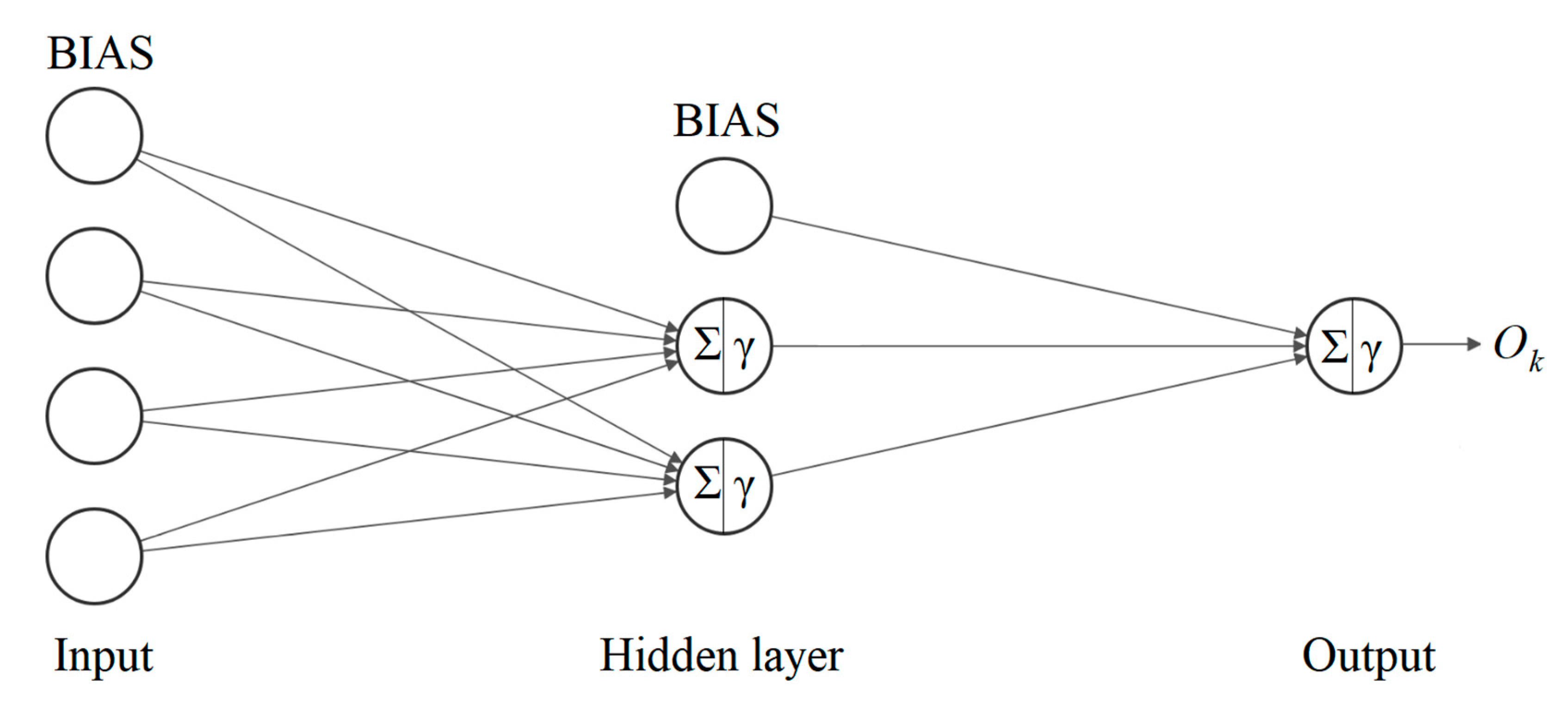
4. Artificial Neural Network Model
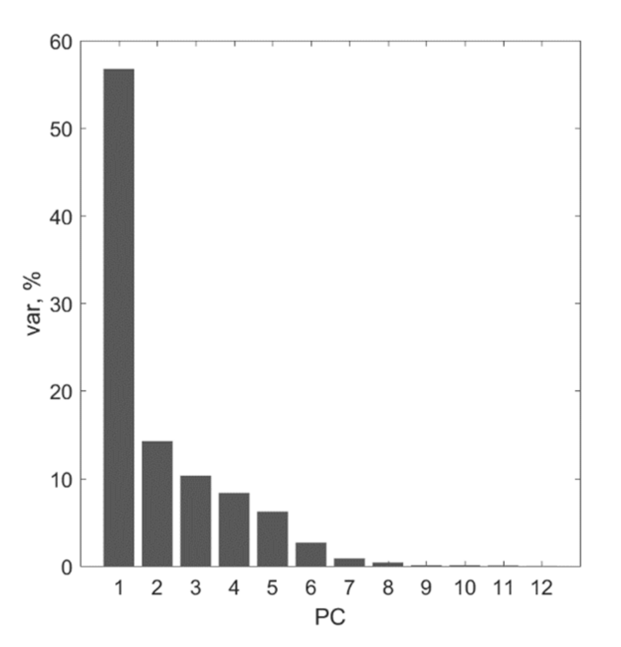
Preparation of Data
5. Results and Discussion
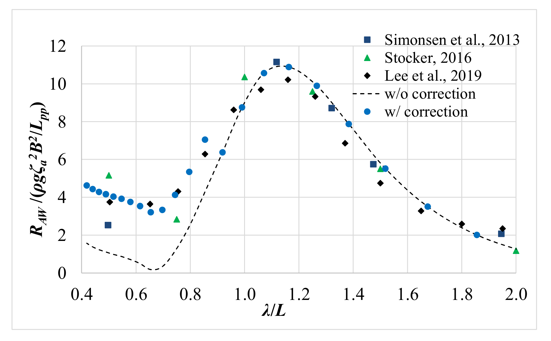
5.1. Validation and Verification of the Numerical Results
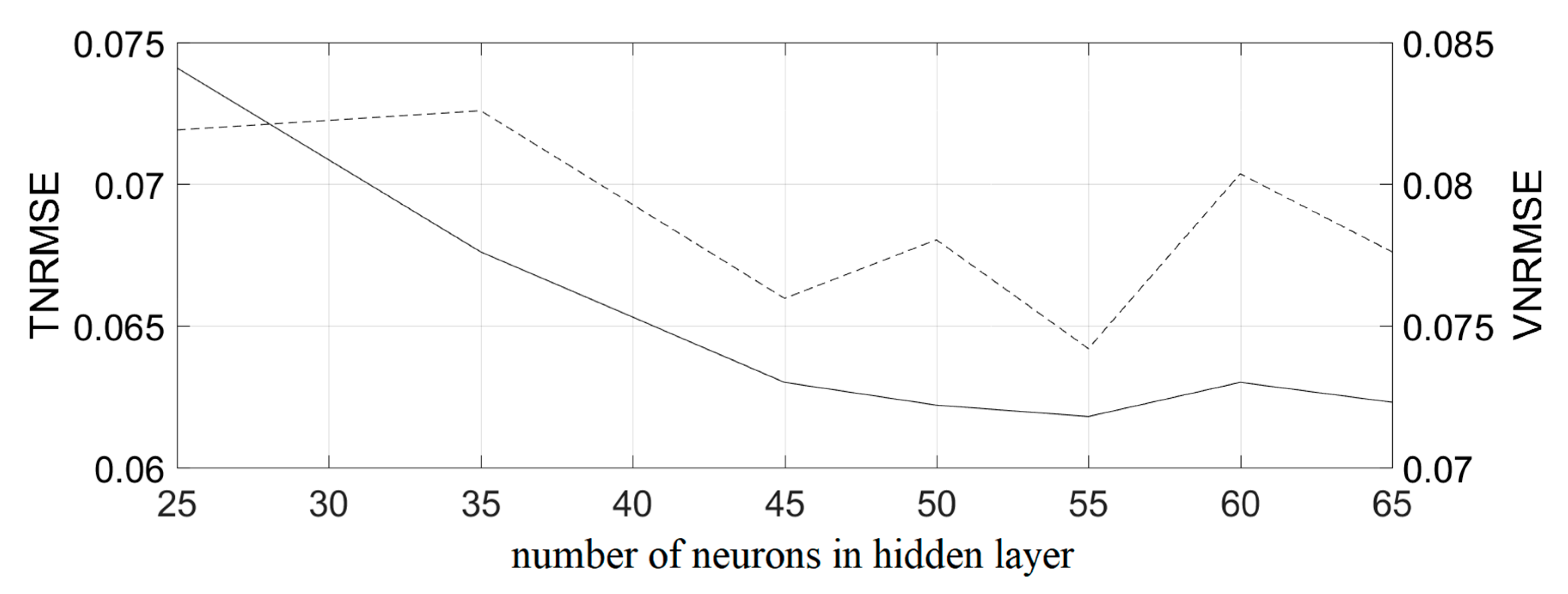
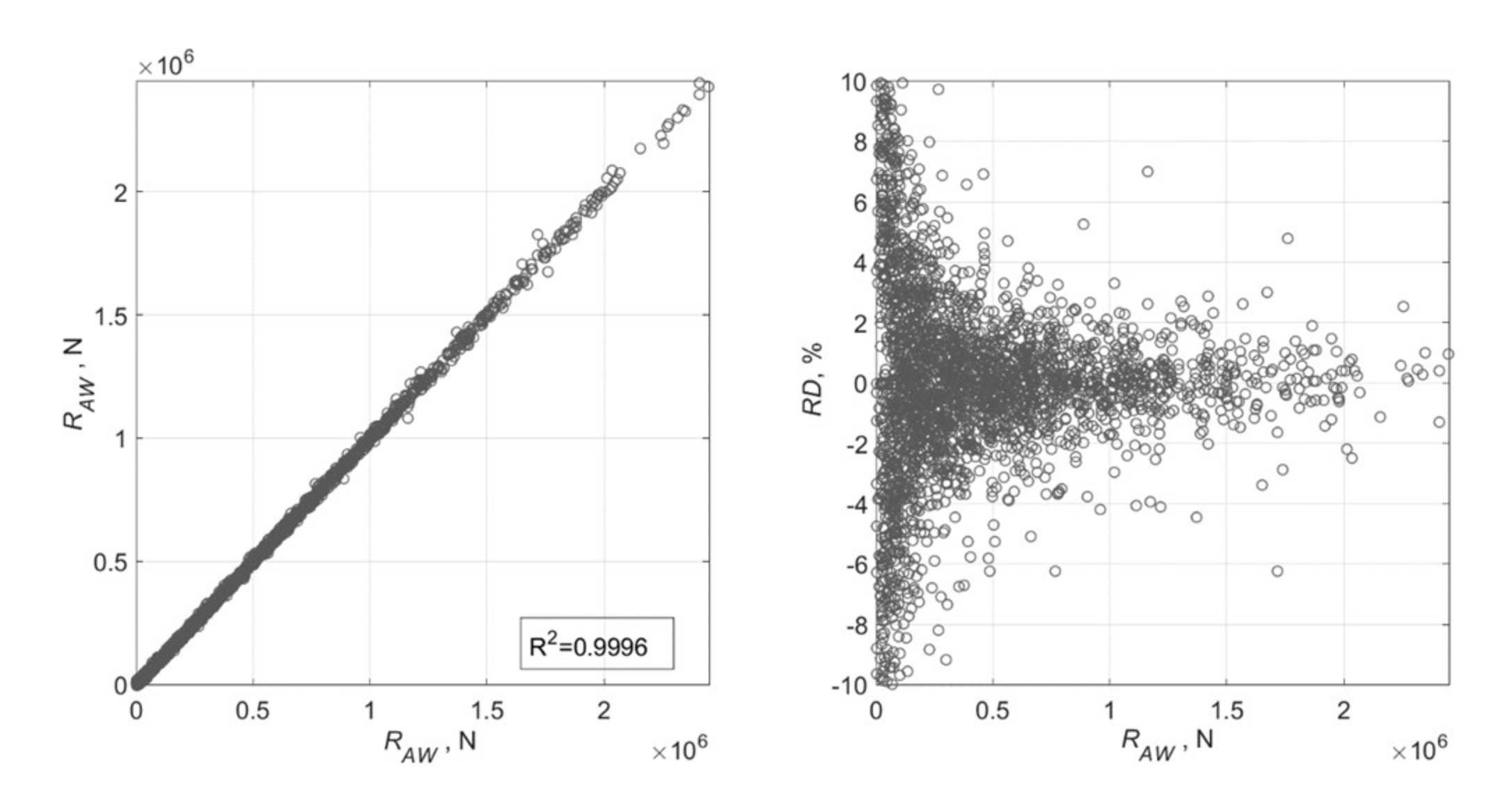
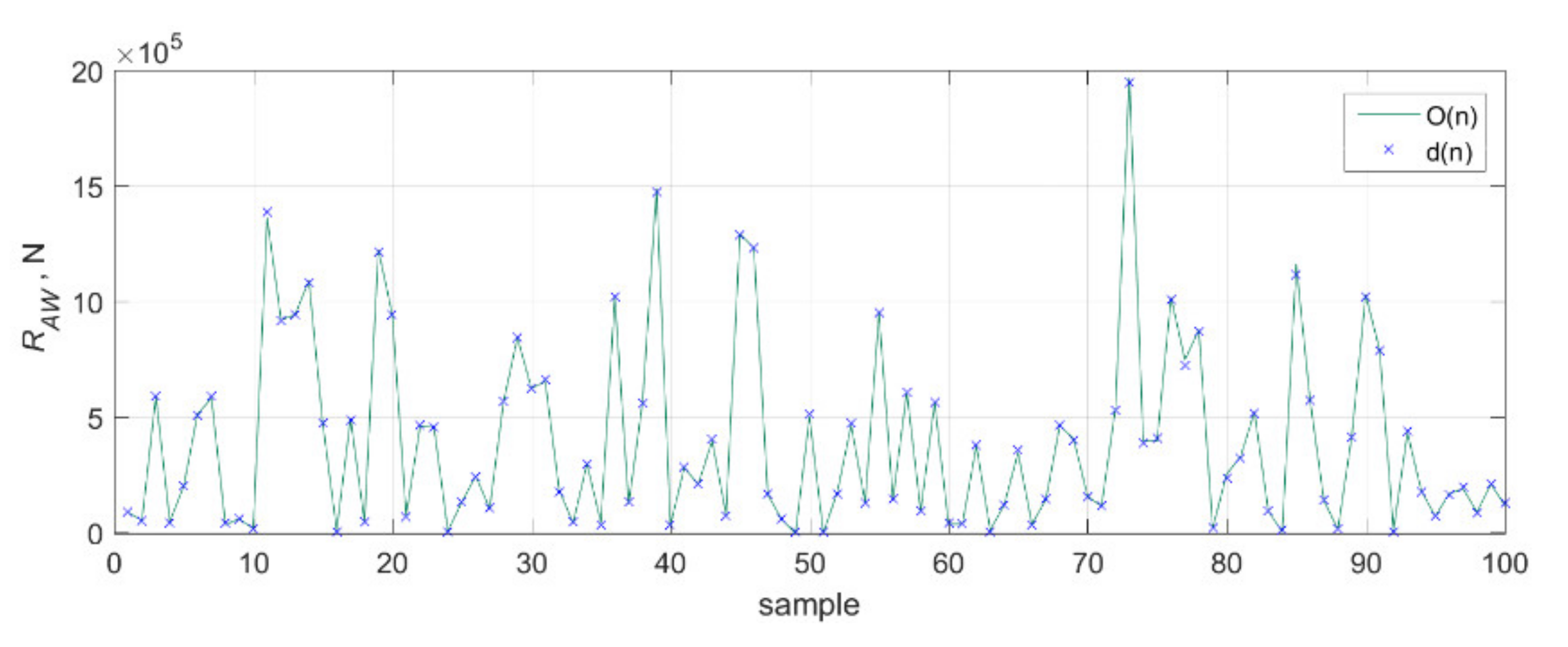
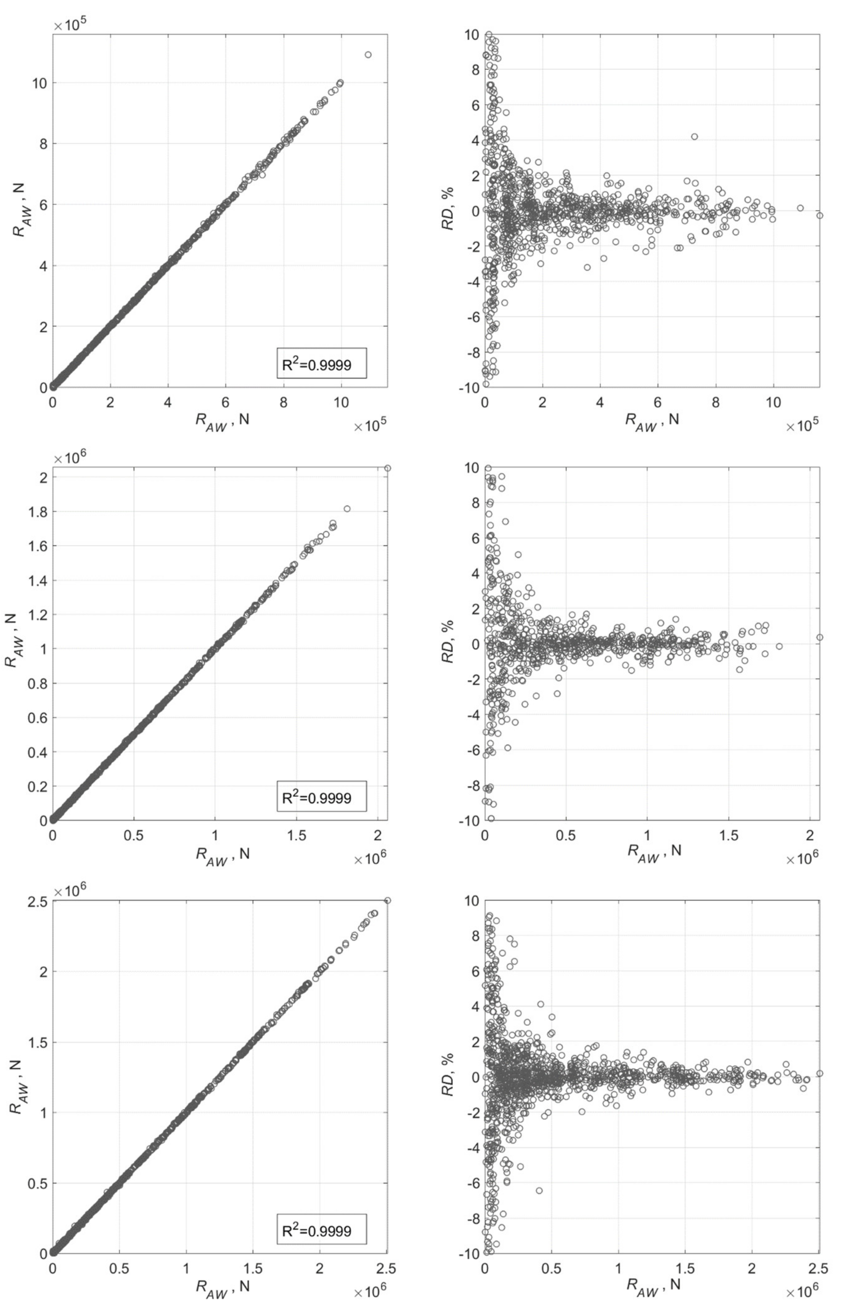
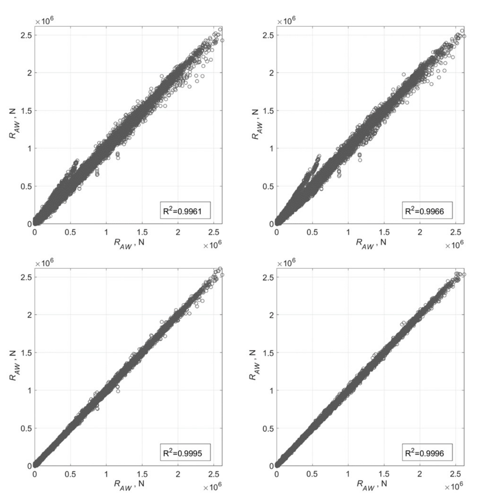
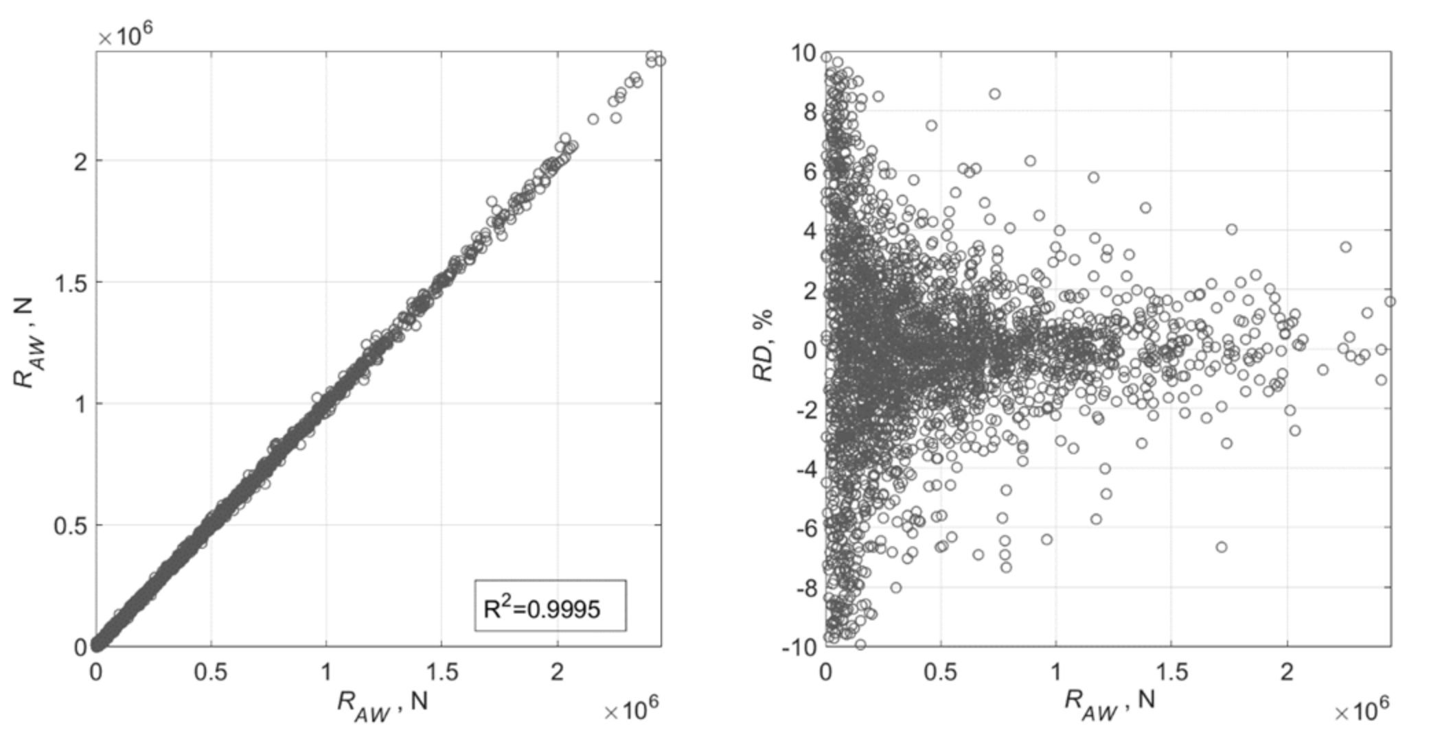
5.2. Results of Artificial Neural Network
6. Conclusions
Author Contributions
Funding
Institutional Review Board Statement
Informed Consent Statement
Data Availability Statement
Acknowledgments
Conflicts of Interest
References
- International Maritime Organization. MARPOL Annex VI MEPC.203(62); International Maritime Organization: London, UK, 2013. [Google Scholar]
- International Towing Tank Conference (ITTC). Recommended Procedures and Guidelines, Seakeeping Experiments, 7.5-02-03-01.5; International Towing Tank Conference (ITTC): Zürich, Switzerland, 2014. [Google Scholar]
- Kim, M.; Hizir, O.; Turan, O.; Incecik, A. Numerical studies on added resistance and motions of KVLCC2 in head seas for various ship speeds. Ocean Eng. 2017, 140, 466–476. [Google Scholar] [CrossRef] [Green Version]
- Youngjun, Y.; Jin Woo, C.; Dong, Y.L. Development of a framework to estimate the sea margin of an LNGC considering the hydrodynamic characteristics and voyage. Int. J. Nav. Archit. Ocean Eng. 2020, 12, 184–198. [Google Scholar]
- Degiuli, N.; Martić, I.; Farkas, A. Environmental aspects of total resistance of container ship in the North Atlantic. J. Sustain. Dev. Energy Water Environ. Syst. 2019, 7, 641–655. [Google Scholar] [CrossRef]
- Degiuli, N.; Martić, I.; Farkas, A.; Gospić, I. The impact of slow steaming on reducing CO2 emissions in the Mediterranean Sea. Energy Rep. 2021. (accepted for publication). [Google Scholar] [CrossRef]
- Sigmund, S.; el Moctar, O. Numerical and experimental investigation of added resistance of different ship types in short and long waves. Ocean Eng. 2018, 147, 51–67. [Google Scholar] [CrossRef]
- Lee, Y.G.; Kim, C.; Park, J.H.; Kim, H.; Lee, I.; Jin, B. Numerical simulations of added resistance in regular head waves on a container ship. Brodogr. Teor. Praksa Brodogr. Pomor. Teh. 2019, 70, 61–86. [Google Scholar] [CrossRef]
- Bunnik, T.; van Daalen, E.; Kapsenberg, G.; Shin, Y.; Huijsmans, R.; Deng, G.; Delhommeau, G.; Kashiwagi, M.; Beck, B. A comparative study on state-of-the-art prediction tools for seakeeping. In Proceedings of the 28th Symposium on Naval Hydrodynamics, Pasadena, CA, USA, 12–17 September 2010. [Google Scholar]
- International Maritime Organization. Interim Guidelines for Determining Minimum Propulsion Power to Maintain the Manoeuvrability of Ships in Adverse Conditions—RESOLUTION MEPC.232(65); International Maritime Organization: London, UK, 2013; Volume 232. [Google Scholar]
- Liu, S.; Papanikolaou, A. Fast approach to the estimation of the added resistance of ships in head waves. Ocean Eng. 2016, 112, 211–225. [Google Scholar] [CrossRef]
- Liu, S.; Papanikolaou, A. Approximation of the added resistance of ships with small draft or in ballast condition by empirical formula. Proc. Inst. Mech. Eng. Part M J. Eng. Marit. Environ. 2019, 233, 27–40. [Google Scholar] [CrossRef]
- Martić, I.; Degiuli, N.; Farkas, A.; Gospić, I. Evaluation of the Effect of Container Ship Characteristics on Added Resistance in Waves. J. Mar. Sci. Eng. 2020, 8, 696. [Google Scholar] [CrossRef]
- Gkerekos, C.; Lazakis, I.; Theotokatos, G. Machine learning models for predicting ship main engine Fuel Oil Consumption: A comparative study. Ocean Eng. 2019, 188, 106282. [Google Scholar] [CrossRef]
- Farag, Y.B.A.; Olçer, A.I. The development of a ship performance model in varying operating conditions based on ANN and regression techniques. Ocean Eng. 2020, 198, 106972. [Google Scholar] [CrossRef]
- Tarelko, W.; Rudzki, K. Applying artificial neural networks for modelling ship speed and fuel consumption. Neural. Comput. Appl. 2020, 32, 17379–17395. [Google Scholar] [CrossRef]
- Kim, J.H.; Kim, Y.; Lu, W. Prediction of ice resistance for ice-going ships in level ice using artificial neural network technique. Ocean Eng. 2020, 217, 108031. [Google Scholar] [CrossRef]
- Im, N.; Nguyen, V. Artificial neural network controller for automatic ship berthing using head-up coordinate system. Int. J. Nav. Archit. Ocean Eng. 2018, 10, 235–249. [Google Scholar] [CrossRef]
- Shuai, Y.; Li, G.; Cheng, X.; Skulstad, R.; Xu, J.; Liu, H. An efficient neural-network based approach to automatic ship docking. Ocean Eng. 2019, 191, 106514. [Google Scholar] [CrossRef]
- Prpić-Oršić, J.; Valčić, M.; Čarija, Z. A Hybrid Wind Load Estimation Method for Container Ship Based on Computational Fluid Dynamics and Neural Networks. J. Mar. Sci. Eng. 2020, 8, 539. [Google Scholar] [CrossRef]
- Awad, T.; Elgohary, M.A.; Mohamed, T.E. Ship roll damping via direct inverse neural network control system. Alex. Eng. J. 2018, 57, 2951–2960. [Google Scholar] [CrossRef]
- Cepowski, T. The prediction of ship added resistance at the preliminary design stage by the use of an artificial neural network. Ocean Eng. 2020, 195, 106657. [Google Scholar] [CrossRef]
- Chen, X. Hydrodynamics in Offshore and Naval Applications—Part I; An updated version of the paper presented as a keynote lecture. In Proceedings of the 6th International Conference on Hydrodynamics, Perth, Australia, 24–26 November 2004; pp. 1–28. [Google Scholar]
- Martić, I.; Degiuli, N.; Farkas, A.; Malenica, Š. Discussions on the convergence of the seakeeping simulations. In Proceedings of the 37th International Conference on Ocean, Offshore & Arctic Engineering, OMAE, Madrid, Spain, 17–22 June 2018; pp. 1–10. [Google Scholar]
- Tsujimoto, M.; Shibata, K.; Kuroda, M.; Takagi, K.A. Practical Correction Method for Added Resistance in Waves. J. Jpn. Soc. Nav. Archit. Ocean Eng. 2008, 8, 177–184. [Google Scholar] [CrossRef] [Green Version]
- International Towing Tank Conference (ITTC). Recommended Procedures and Guidelines, Seakeeping Experiments, 7.5-02-07-02.1; International Towing Tank Conference (ITTC): Zürich, Switzerland, 2014. [Google Scholar]
- International Towing Tank Conference (ITTC). Recommended Procedures and Guidelines, Verification and Validation of Linear and Weakly Nonlinear Seakeeping Computer Codes 7.5-02-07-02.5; International Towing Tank Conference (ITTC): Zürich, Switzerland, 2011. [Google Scholar]
- International Towing Tank Conference (ITTC). Recommended Procedures and Guidelines, Uncertainty Analysis in CFD Verification and Validation, Methodology and Procedures 7.5-03-01-01; International Towing Tank Conference (ITTC): Zürich, Switzerland, 2017. [Google Scholar]
- Hizir, O.; Kim, M.; Turan, O.; Day, A.; Incecik, A.; Lee, Y. Numerical studies on non-linearity of added resistance and ship motions of KVLCC2 in short and long waves. Int. J. Nav. Archit. Ocean Eng. 2019, 11, 143–153. [Google Scholar] [CrossRef]
- Eca, L.; Hoekstra, M. An Evaluation of Verification Procedures for CFD Applications. In Proceedings of the 24th Symposium on Naval Hydrodynamics, Fukuoka, Japan, 8–13 July 2002; pp. 8–13. [Google Scholar]
- Eca, L.; Vaz, G.B.; Falcao de Campos, J.A.C.; Hoekstra, M. A verification of calculations of the potential flow around 2D foils. AIAA J. Am. Inst. Aeronaut. Astronaut. 2004, 42, 2401–2407. [Google Scholar] [CrossRef]
- United Nations. Review of Maritime Transport 2019; United Nations: New York, NY, USA, 2019. [Google Scholar]
- United Nations. UNCTADSTAT. Available online: https://unctadstat.unctad.org/wds/TableViewer/tableView.aspx (accessed on 5 July 2021).
- International Maritime Organization. Fourth IMO Greenhouse Gas Study 2020; International Maritime Organization: London, UK, 2020. [Google Scholar]
- DELFTship v11.20; Delftship BV: Hoofddorp, The Netherlands, 2019.
- Martić, I.; Degiuli, N.; Komazec, P.; Farkas, A. Influence of the approximated mass characteristics of a ship on the added resistance in waves. In Proceedings of the IMAM 2017, 17th International Congress of the International Maritime Association of the Mediterranean, Maritime Transportation and Harvesting of Sea Resources, Lisabon, Portugal, 9–11 October 2017. [Google Scholar]
- Kristensen, H.O. Statistical Analysis and Determination of Regression Formulas for Main Dimensions of Container Ships Based on IHS Fairplay Data; Project no. 2010-56, Report; Technical University of Denmark: Kongens Lyngby, Denmark, 2013. [Google Scholar]
- Papanikolaou, A. Ship Design, Methodologies of Preliminary Design; Springer: Berlin/Heidelberg, Germany, 2014. [Google Scholar]
- Lackenby, H. On the systematic geometrical variation of ship forms. Trans. Inst. Nav. Archit. 1950, 92, 289–315. [Google Scholar]
- Hagan, M.T.; Demuth, H.B.; Beale, M.H. Neural Network Design; PWS Publishing: Boston, MA, USA, 1996. [Google Scholar]
- Hagan, M.T.; Menhaj, M.B. Training Feedforward Networks with the Marquardt Algorithm. IEEE Trans. Neural Netw. 1994, 5, 989–993. [Google Scholar] [CrossRef] [PubMed]
- Moller, M.F. A Scaled Conjugate Gradient Algorithm for Fast Supervised Learning. Neural Netw. 1993, 6, 525–533. [Google Scholar] [CrossRef]
- MacKay, D.J. Bayesian interpolation. Neural Comput. 1992, 4, 415–447. [Google Scholar] [CrossRef]
- Simonsen, C.D.; Otzen, J.F.; Joncquez, S.; Stern, F. EFD and CFD for KCS heaving and pitching in regular head waves. J. Mar. Sci. Technol. 2013, 18, 435–459. [Google Scholar] [CrossRef]
- Stocker, M.R. Surge Free Added Resistance Tests in Oblique Wave Headings for the KRISO Container Ship Model; University of Iowa: Iowa, IA, USA, 2016. [Google Scholar]
- Lee, C.; Park, S.; Yu, J.; Choi, J.; Lee, I. Effects of diffraction in regular head waves on added resistance and wake using CFD. Int. J. Nav. Archit. Ocean Eng. 2019, 11, 736–749. [Google Scholar] [CrossRef]


| Main Particular | Value |
|---|---|
| , m | 230 |
| , m | 32.2 |
| , m | 10.8 |
| , m3 | 52,030 |
| 0.651 | |
| , m2 | 9530 |
| , % | −1.48 |
| , m | 111.6 |
| , m | 7.28 |
| 0.40 | |
| 0.25 | |
| , kn | 24 |
| Ship | , m | , m | , m3 | |||||
|---|---|---|---|---|---|---|---|---|
| CS1 | 319 | 42.8 | 13 | −3.49 | 0.9682 | 0.5907 | 0.6100 | 104,841.9 |
| CS2 | 153 | 25 | 8 | −0.691 | 0.9836 | 0.6583 | 0.6693 | 21,357.9 |
| CS3 | 132 | 21.5 | 7 | −0.691 | 0.9836 | 0.6583 | 0.6693 | 13,865.9 |
| CS4 | 247 | 32.26 | 12 | −2.438 | 0.9589 | 0.6057 | 0.6316 | 61,018.5 |
| CS5 | 178 | 25.85 | 9 | −0.849 | 0.9598 | 0.5853 | 0.610 | 24,457.2 |
| CS6 | 234 | 32.42 | 11.25 | −1.464 | 0.9506 | 0.6812 | 0.7166 | 59,445.3 |
| CS7 | 106 | 20.3 | 4.25 | 0.138 | 0.9622 | 0.7146 | 0.7426 | 6221.82 |
| CS8 | 104.8 | 18 | 7.9 | −0.499 | 0.9697 | 0.6173 | 0.6366 | 9937.3 |
| CS9 | 155.4 | 23.3 | 9.2 | −1.683 | 0.9878 | 0.5619 | 0.5689 | 19,473.8 |
| CS10 | 300 | 37 | 11 | −2.963 | 0.9305 | 0.5292 | 0.5687 | 67,244 |
| CS11 | 196 | 28 | 8.5 | −1.614 | 0.9622 | 0.5721 | 0.5946 | 26,687.6 |
| CS12 | 120.7 | 19 | 7.5 | −0.886 | 0.9824 | 0.6682 | 0.6802 | 12,537.6 |
| CS13 | 215 | 27 | 8 | −0.216 | 0.9769 | 0.7097 | 0.7265 | 34,808 |
| CS14 | 360 | 49 | 15 | −1.137 | 0.9632 | 0.5830 | 0.6053 | 164,760.5 |
| CS15 | 340 | 44 | 15 | −2.438 | 0.9588 | 0.6100 | 0.6360 | 143,199.6 |
| 2.0 | 1.518 | 1.513 | 1.492 | 4.4882 | / | / | / | / |
| 1.5 | 6.326 | 6.244 | 6.221 | 0.2911 | 1.7803 | 0.0098 | 6.211 | 0.197 |
| 1.33 | 9.193 | 9.069 | 8.989 | 0.6483 | 0.6252 | 0.1484 | 8.840 | 2.098 |
| 1.15 | 11.279 | 10.996 | 10.718 | 0.9828 | / | / | / | / |
| 0.5 | 0.780 | 0.762 | 1.568 | −43.1464 | / | / | / | / |
| 10.813 | 10.578 | 10.455 | 0.5238 | 0.9329 | 0.1353 | 10.320 | 1.639 |
| Learning Algorithm | SGD | LM | SCG | BR | |||
|---|---|---|---|---|---|---|---|
| Error | TNRMSE | VNRMSE | TNRMSE | VNRMSE | TNRMSE | VNRMSE | TNRMSE |
| Norm. data 1 | 0.0624 ) | 0.0766 ) | 0.0231 | 0.0239 | 0.0583 | 0.0589 | 0.0231 |
| 0.0615 ) | 0.0756 ) | ||||||
| 0.0613 ) | 0.0736 ) | ||||||
| 0.0647 ) | 0.0703 ) | ||||||
| Stand. data 2 | 0.0633 ) | 0.0772 ) | 0.0238 | 0.0246 | 0.0581 | 0.0585 | 0.0238 |
| 0.0616 ) | 0.0757 ) | ||||||
| 0.0618 ) | 0.0742 ) | ||||||
| 0.0665 ) | 0.0725 ) | ||||||
| PCA data | 0.0639 ) | 0.0792 ) | 0.0234 | 0.0236 | 0.0545 | 0.0559 | 0.0204 |
| 0.0628 ) | 0.0788 ) | ||||||
| 0.0619 ) | 0.0774 ) | ||||||
| 0.0670 ) | 0.0804 ) | ||||||
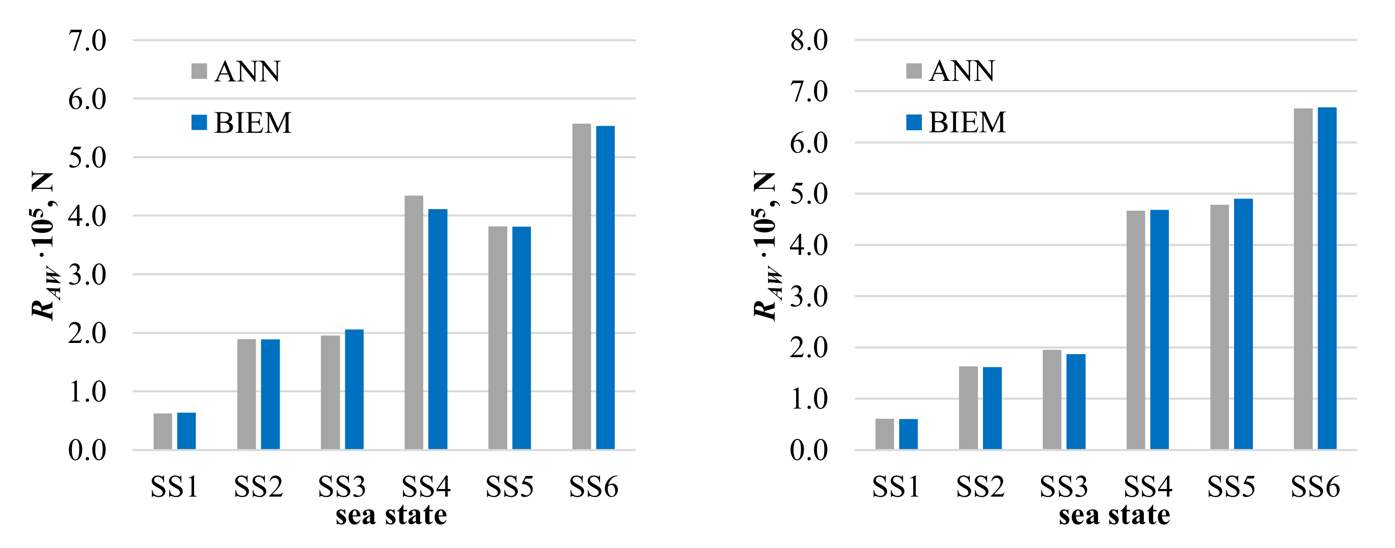
| Sea State | ||
|---|---|---|
| SS1 | 1.5 | 6.5 |
| SS2 | 2.5 | 7.5 |
| SS3 | 2.5 | 8.5 |
| SS4 | 3.5 | 9.5 |
| SS5 | 3.5 | 10.5 |
| SS6 | 4.5 | 11.5 |
| Sea State | SS1 | SS2 | SS3 | SS4 | SS5 | SS6 |
|---|---|---|---|---|---|---|
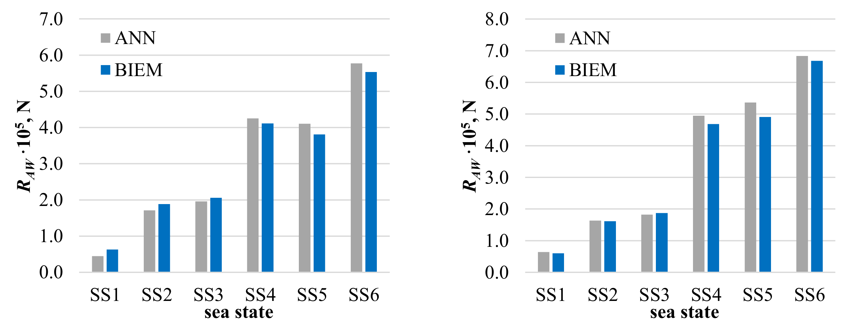
| Bretschneider | −18,871.77 N (−29.74%) | −17,570.78 N (−9.32%) | −9839.05 N (−4.78%) | 14,353.20 N (3.49%) | 29,563.43 N (7.76%) | 23,951.34 N (4.33%) |
| JONSWAP | 4175.82 N (6.95%) | 1610.69 N (1.00%) | −5053.55 N (−2.70%) | 26,480.53 N (5.66%) | 45,777.20 N (9.34%) | 15,146.23 N (2.27%) |
| Sea State | SS1 | SS2 | SS3 | SS4 | SS5 | SS6 |
|---|---|---|---|---|---|---|
| Bretschneider | −979.25 N (−1.54%) | 412.74 N (0.22%) | −10,368.66 N (−5.04%) | 23,358.19 N (5.68%) | 413.40 N (0.11%) | 3841.04 N (0.69%) |
| JONSWAP | 930.11 N (1.55%) | 1258.65 N (0.78%) | 8318.72 N (4.45%) | −1038.39 N (−0.22%) | −11,775.83 N (−2.40%) | −1692.20 N (−0.25%) |
Publisher’s Note: MDPI stays neutral with regard to jurisdictional claims in published maps and institutional affiliations. |
© 2021 by the authors. Licensee MDPI, Basel, Switzerland. This article is an open access article distributed under the terms and conditions of the Creative Commons Attribution (CC BY) license (https://creativecommons.org/licenses/by/4.0/).
Share and Cite
Martić, I.; Degiuli, N.; Majetić, D.; Farkas, A. Artificial Neural Network Model for the Evaluation of Added Resistance of Container Ships in Head Waves. J. Mar. Sci. Eng. 2021, 9, 826. https://doi.org/10.3390/jmse9080826
Martić I, Degiuli N, Majetić D, Farkas A. Artificial Neural Network Model for the Evaluation of Added Resistance of Container Ships in Head Waves. Journal of Marine Science and Engineering. 2021; 9(8):826. https://doi.org/10.3390/jmse9080826
Chicago/Turabian StyleMartić, Ivana, Nastia Degiuli, Dubravko Majetić, and Andrea Farkas. 2021. "Artificial Neural Network Model for the Evaluation of Added Resistance of Container Ships in Head Waves" Journal of Marine Science and Engineering 9, no. 8: 826. https://doi.org/10.3390/jmse9080826
APA StyleMartić, I., Degiuli, N., Majetić, D., & Farkas, A. (2021). Artificial Neural Network Model for the Evaluation of Added Resistance of Container Ships in Head Waves. Journal of Marine Science and Engineering, 9(8), 826. https://doi.org/10.3390/jmse9080826