Article

The Effect of Mesoscale Eddy on the Characteristic of Sound Propagation

1
Acoustic Science and Technology Laboratory, Harbin Engineering University, Harbin 150001, China
2
Key Laboratory of Marine Information Acquisition and Security, Ministry of Industry and Information Technology, Harbin Engineering University, Harbin 150001, China
3
College of Underwater Acoustic Engineering, Harbin Engineering University, Harbin 150001, China
*
Author to whom correspondence should be addressed.
J. Mar. Sci. Eng. 2021, 9(8), 787; https://doi.org/10.3390/jmse9080787
Submission received: 15 June 2021 / Revised: 9 July 2021 / Accepted: 17 July 2021 / Published: 22 July 2021
(This article belongs to the Special Issue Sea Level Fluctuations)

Abstract

:
A mesoscale eddy is detected and tracked in the western North Pacific region. Within the life cycle of the cyclonic eddies, the intensities of eddies make a difference. Satellite images indicate the oceanic eddy keeps westward-moving until it disappears. Oceanographic and acoustic characteristics of the eddy are studied. The acoustic energy distribution results from the different intensity of both modelled eddy and measured eddy are calculated. With sound propagation through the cyclonic eddy and anticyclonic eddy, the position of convergence zone moves away from and towards the acoustic source compared with the sound propagation through background hydrography. The coupling coefficient of different orders of normal modes changes significantly. The closer to the centre of the eddy, the stronger the coupling coefficient.

1. Introduction

Ocean dynamic phenomena have been distributed in the global ocean. Among them, eddies are characterised by unstable, time-dependent water masses, which separate from their respective currents and enter water bodies with different physical, chemical and biological characteristics [1]. More than half of the kinetic energy of the ocean circulation is stored in the mesoscale eddies, with the remainder contained in the large-scale circulation, swirling motions of eddies mixed between layers and consequent mixing of nutrients, heat and salinity. Sound propagation through eddies has a crucial impact on humans, marine animals and invertebrates [2]. Under the influence of oceanic eddies, human underwater acoustic communication networks are impacted. The existence of eddies affects the detection and communication of marine creatures [3]. Some whales, seals and fishes use low-frequency sound to communicate, perceive the environment and respond to those sounds [4]. At present, there are some experiments to prove that the sound of deep-sea creatures is detected at a location of 15 km away. Fishes feed along with the density structure of the eddies, which indicates that eddies accelerate the transfer of energy and nutrients in the ocean. Anticyclonic eddies carry higher surface chlorophyll than cyclonic eddies. Because the mixed layer of cyclonic eddies is often shallower than that of anticyclonic eddies, the pycnocline depth of the anticyclonic eddies is deeper. More plankton in the deeper mixed layer therefore provides more nutrients for zooplankton [5]. The study of sound propagation through the eddies clearly plays a significant role in the life of human and marine organisms. Regarding the deep-sea sound propagation issue, we always focus on the convergent position of sound energy and the acoustic intensity distribution. Aiming at the phenomenon of how the oceanic eddy affects the position of the convergence zone, this paper uses the parabolic equation method to solve sound field and combines it with the normal mode theory to analyse the difference of energy distribution of the acoustic wave at different positions.
It is of great significance for weather and marine scientific research to grasp the real-time movement of eddies. The nonlinear interaction of barotropic and baroclinic Rossby waves could lead to strong instability, which is a major source of the kinetic energy of eddies [6]. These eddies are affected by Coriolis, which lifts high-temperature cyclones from subsurface water to the surface of the sea [
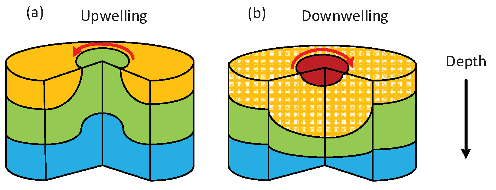
7]. Some smaller-scale eddies (tens of kilometres in diameter) are formed due to the instability of baroclinic at the horizontal density, while larger-scale eddies located near the warm current of Gulf Stream and the Kuroshio Current are generally due to strong horizontal shear motion, which intensely affects the temperature and salinity distribution in the depth direction. The dynamic model of the eddies was proposed as early as the 19th century. Taking the change of sea surface height and the temperature in the depth direction caused by the eddies into account, the sound speed shapes in space can be divided into the following types: bowl shape, lens-shaped, cone-shaped, moreover, the generation mechanism of eddies are divided into three types, sea surface wind, the interaction between ocean currents and bottom topography, and Kuroshio intrusion [8]. In the northern hemisphere, these cyclonic eddies rotate clockwise, whereas, in the southern hemisphere, they rotate counterclockwise. The low-temperature anticyclonic eddies cause the downwelling of the surface layer and dent formed in opposite directions of rotation. Eddies could be distinguished through the combination of sea surface height and sea surface temperature anomalies. Some scholars used buoys to capture the formation, the movement and the extinction of eddies. Mesoscale eddies in the Pacific generally last several weeks. Their motion trajectories are approximately circular with a diameter of 100–200 km. The effect of the mesoscale eddies gradually concerns many scholars and has great investigation result. The oceanic eddies not only affect the circulation structure of the ocean but also ocean temperature, salinity, sound speed profile. Mesoscale eddies keep rotating and moving every moment, and momentum and energy are transported, interacting strongly with oceanic circulations, affecting the vertical profile structure of the marine environment. In 1977, based on practical experience, Henrick proposed a quasi-elliptical eddy model. To detect and track mesoscale eddies [9], Dong used sea surface height fluctuations to study the distribution laws and characteristics of eddies from the perspective of oceanography [10]. We study from the perspective of ocean acoustics the influence of spatial and temporal distribution characteristics of eddies.
Since the 1970s, hydro-acoustics scientists have been concerned about the influence of ocean eddies on sound propagation. The ray method is used for analysing the receiver’s time of arrival which is affected by the size, intensity and position of the eddy. By using the ray-tracing model, people could understand how rays refract and bend. Additionally, what people tracing is the ray stimulated from a particular source then propagating in free space [11]. In the classical ray theory, the sound energy in the waveguide is shown in the form of acoustic rays. With regards to sound rays from the point source traveling along certain paths to the receiving point, the acoustic field at the receiver is the consequence of the superposition of all types of sound rays. Furthermore, the receivers’ signal phase shift is also calculated by Jian [12] combining the current model with the acoustic field model when an eddy is present. In addition to the frequency domain, scholars have also done some research on sound propagation through the eddies. Nysen [13,14] studied how the acoustic energy leaked into the deep sound channel from the subsurface sound channel with the dependence of frequency off the east coast of Australia. The strong coupling between the two ducts leads to the near-surface acoustic energy being trapped in the duct area affected by water mass. Lawrence [15] modelled a warm-core eddy propagation problem and expounded the widening of the acoustic convergence zone. Baer [16] bonded split-step parabolic-equation and used Henrick eddy model to calculate a non-typical three-dimensional structure of eddy and examined the signal amplitude of vertical line array. Specifically, the gain of the hydrophone array increased, and the energy flows horizontal angle changed by over 0.5 degrees. As underwater acoustic horizontal refraction has attracted attention because of the eddy, Weinberg [17] simulated acoustic propagation through ocean fronts and single mesoscale eddy. The received voltage amplitude was significantly dependent upon the position of the Gulf Stream ring by a fixed system experiment. Afterwards, the three-dimensional fully coupled parabolic equation method was applied to investigate the effect of the horizontal refraction of the sound field caused by mesoscale ocean dynamics on the impact of acoustic source localisation [18].
Even though the parabolic equation and the ray method could solve the sound field problem of horizontal ocean environment fluctuations, the normal mode theory still plays an irreplaceable role of analysing the effect of deep-sea eddies on the sound field. Dozier and Tapert [19] deduced the normal mode amplitude distribution in a random ocean, Colosi [20] used the coupling coefficient of acoustic normal mode to analyse the average energy and sound pressure correlation characteristics of sound propagation under the influence of internal waves. Similarly, we use the coupling coefficient derived by Tapert to apply it to the ocean environment with an eddy to analyse the coupling relationship of the normal mode of various orders in the deep ocean environment. As the sea depth increases, the total of normal mode order increases. The theory of deep-sea normal modes is more complicated than that of shallow-sea. High-order normal mode of the energy coupling is more intense, according to the simulation results. Consistent with the coupling and transmission characteristics of shallow sea normal mode, however, as the sound source is located far away from the channel axis and closer to the sea surface, the low-order normal mode no longer maintains a stable propagation path over a long distance. As a consequence, we focus on the energy distribution of higher-order normal modes in the deep sea. Incidentally, due to the surface and seabed boundary limitation of the impedance character, the confined depth direction is expressed as a specific form of a standing wave, whereas the unconfined direction is known as a form of a travelling wave, which is called normal mode in a given waveguide. The modal expansion is a sum of resonances or eigenfunctions for the waveguide. The eigenfunction mentioned here is limited to the formal solution of the Helmholtz equation under the conditions of a given waveguide section and a fixed edge condition, and eigenfunction, namely, mode shape function expansion is often done in the numerical models based on the normal mode approach [11]. Local eigenfunctions of different positions are used to analyse the redistribution of energy of the normal mode of each order in the eddy affecting the sound field and explain the root cause of the change of the convergence zone position. As follows in Section 2, an eddy environment was tracked and used to resolve the sound propagation and the forecasting process of the sound transmission based on the parabolic equation method, and then, the sound propagation experiments in the Kuroshio are introduced, and the comparison between the measured results and numerical results is carried out in Section 3. In Section 4, the numerical results of the modelled cyclonic and anticyclonic eddies acoustic propagation and coupling characteristics are described, the character of sound propagation of different normal modes is analysed. Summary of the discussions is drawn in Section 5.

2. Materials and Methods

2.1. Gaussian Eddy Hydrology Model

In the deep ocean, the speed of sound varies between 1450 and 1570 m per second. Notably, sound speed profiles have a remarkable influence on the variation of the temperature and salinity which is associated with eddies. Specifically, the intensity of eddy represents the difference between the acoustic properties at the eddy edge and eddy centre. Its intensity does also reflect how surface cool water rises or how deeply warm water descends. The upwelling and downwelling of the eddy (as shown in the Figure 1) could be simplified as an asymmetric model with Gaussian distribution. The temperature/salinity profile for a cold-core or warm-core eddy could be simply modelled as (referring to the theory section of [21,22]):
T ( r , z ) = T k ( z ) ( 1 e ( r R ) ) + T c ( z ) e ( r R ) ,
where T k is the background value of temperature/salinity without eddy, and T c is the value of temperature/salinity of an eddy core. Typically, R = 3 R 0 , where R 0 is the radius of Rossby. Particular temperature and salinity formulation for an elliptical eddy feature model is simplified given by
T ( r , z ) = T c ( z ) α β ( r ) ,
where α is generally a delta function, β ( r ) is an exponential function depending on the current characteristic. The empirical formula of sound speed profile could be determined by temperature and salinity. Gaussian eddy sound speed model has an advantage in considering underwater sound propagation related issues, and the overall sound speed is distributed as
c ( r , z ) = c 0 ( z ) + δ c ( r , z ) = c 0 ( z ) + D C e x p ( ( r r 0 d r ) 2 ( z z 0 d z ) 2 )
where D C is the amplitude of variation of sound speed because of the existence of the eddy, r 0 and z 0 are the location of the core of eddy and d r and d z are the radius of semi-major axis and radius of semi-axis of eddy, respectively. Otherwise, background sound speed satisfies the Munk deep ocean sound speed profile, where c 0 ( z ) = 1500 ( 1 + 0.0057 ( e ζ ( 1 ζ ) ) ) , z c 0 is the depth of the sound channel axis in the equation ζ = 2 ( z z c 0 ) z c 0 .

2.2. Parabolic Equation Modelling

To solve range dependent propagation problem for low-frequency sound propagation, a more appropriate model is the parabolic equation. The acoustical wave equation can be derived as serial spatial iterative equations [23,24,25]. Previously, we start with the Helmholtz equation with a point source for constant density sediment:
2 P r 2 + 1 r P r + ρ z 1 ρ P z + k 2 P = 0
where k = ω c = ω c 0 n = k 0 n , k 0 is defined as reference wave number, ω is the angular frequency, c is the sound speed, c 0 is the reference sound speed of 1500 m per second, and n is the index of refraction. Simulating the acoustic field by frequency-domain finite difference method, selecting and keeping only the outgoing sound pressure component we consequently obtain
[ ϕ H 0 ( 1 ) ( k 0 r ) ] r = i k 0 1 + X [ ϕ H 0 ( 1 ) ( k 0 r ) ]
P = ϕ H 0 ( 1 ) ( k 0 r ) , where H 0 ( 1 ) is zeroth-order Hankel function of the first kind, which satisfies the Bessel differential equation. Then it is displayed in the iterative form, ϕ ( r + r ) = e i k 0 r 1 + X ϕ ( r ) , where operator X = 1 k 0 2 [ 1 α ( z ) z ( α ( z ) z ) + k 2 k 0 2 ]
This approximation equation is a one-way wave equation that could be estimated step by step in the recursion. Eventually, sound transmission loss is decibel quantities
T L = 20 l g P p 0 ( r = 1 )
where p 0 is the pressure of the source in the free space. For a smoothed transmission loss result ( j = 1 J P ( r , z ) 2 ) 1 / 2 , where J is the total number of wide-band covered frequency points.

2.3. Normal Mode Method

For the purposes of acquiring the primary causes of the redistribution of the sound energy, the mode decomposition method is applied. According to normal mode theory [11,26], the sound field is represented as the superposition of the normal modes.
P ( r , z ) = n = 1 a n ( r ) ϕ n
where ϕ n are eigenfunctions of depth separated equations, and a n ( r ) is amplitude of range dependence. The orthogonal property of ϕ n is represented as
0 D ϕ n ϕ m ρ d z = δ n m
By multiplying local eigenfunctions to both sides of Equation (8), the amplitude distributions of different orders of normal modes are solved after integrating with the total depth direction. We then obtain the following form:
0 D p ( r , z ) ϕ m ( z ) d z = 0 D n = 1 N a n ( r ) ϕ n ( z ) ϕ m ( z ) d z
To illustrate the effect of coupling between normal modes of each order, putting 7 into formation wave Equation (4) we obtained
n = 1 N ( ω 2 c 2 a n ( r ) ϕ n ( z ) + 2 a n ( r ) r 2 ϕ n + a n ( r ) 2 ϕ n ( z ) z 2 ) = 0
The form expressed as a potential function is 2 ϕ n ( z ) z 2 = ( k n 2 k 0 2 ) ϕ n ( z ) , where k n is horizontal wave number of nth normal mode. The above formula is reorganised and obtained as follows,
n = 1 N ( ω 2 c 2 a n ( r ) ϕ n ( z ) + 2 a n ( r ) r 2 ϕ n + a n ( r ) ( k n 2 k 0 2 ) ϕ n ( z ) ) = 0
The orthogonal property of eigenfunction is used, and as a result we get
2 a n ( r ) r 2 + a n ( r ) k n 2 + m 1 M B n m ( r , t ) a m ( r ) = 0
The coupling coefficient is described as
B m n ( r , t ) = 2 ω 2 c 0 2 0 D δ c ( r , z ) c 0 ϕ n ( z ) ϕ m ( z ) d z
The range dependent amplitude component is obtained by using small angle single scattering approximation
a n z i k n a n = i n = 1 N B n m ( r ) a m
The expression of coupling coefficient of the stochastic ocean is obtained
B m n = k 0 2 k n k m 0 D δ c ( r , z ) c 0 ϕ n ( z ) ϕ m ( z ) d z

3. Eddy Tracking Experiments and Underwater Acoustic Propagation Experiment

From May to July 2019, a joint acoustic propagation/mesoscale eddy physics experiment was carried out near the Kuroshio. The purposes of the experiment were to explore eddy hydrology structure and the influence of eddy on sound propagation. The expendable conductivity temperature depth (XCTD), conductivity temperature depth (CTD) and moving vessel profiler (MVP) were used to measure temperature and salinity in the ocean. Observational networks were extended to cover practically the entire mesoscale eddy area, a longitude from 148.5° E to 150.5° E and latitude from 33.65° N to 34.15° N. Receiver hydrophone line array coordinate is located at 150°30 E, 33°42 
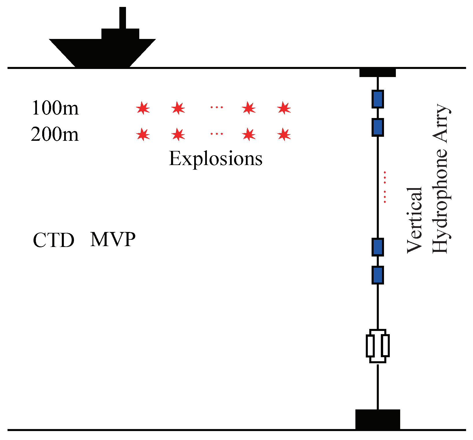
N. Moreover, the survey depth fluctuates obviously from 5900 to 6040 m. The surface sound speed approximately is 1520 m/s; the sound speed at the lowest channel axis position is 1484 m/s and increases to around 1547 m/s near the seabed. The equipment used for the experiment is shown in Figure 2 to track and measure the distribution of sound speed which lasted four days since 16 June 2019. Two types of explosives were selected whose explosion depth is 100 m and 200 m, respectively. The deep-sea sound propagation experiment was conducted by 1 kg explosions, dropped evenly spaced at the constant latitude and along the direction of longitude. The broadband explosive was occurring every 3 km, and the ship sailing within 3 h at a speed of 5 knots on the survey line. Inasmuch as the impact of ocean currents, two depth meters are hung on the vertical hydrophone line array to determine the position of each hydrophone in actual time.
With the influence of sea conditions, the depth of the receiving hydrophones fluctuates up and down. After the depth of hydrophones is determined through depthometers, the signal of sound pressure at the same depths is corrected. The sampling frequency is 10 kHz. To guarantee the integrity of the received signal, the time window for intercepting the signal is selected according to the actual signal amplitude. What is more, the signal spectrum is distributed at 5–500 Hz. In a practical process of data processing, 320 Hz with the strongest received signal spectrum is truncated for one-third octave band filtering to process the voltage signal. The parabolic equation method is used for calculating the sound intensity at the receiving position, and the broadband average sound intensity is achieved by averaging the frequency points within the bandwidth to ensure the consistency of the processing result of the experiment and the propagation loss curve.

3.1. Hydrographic Data

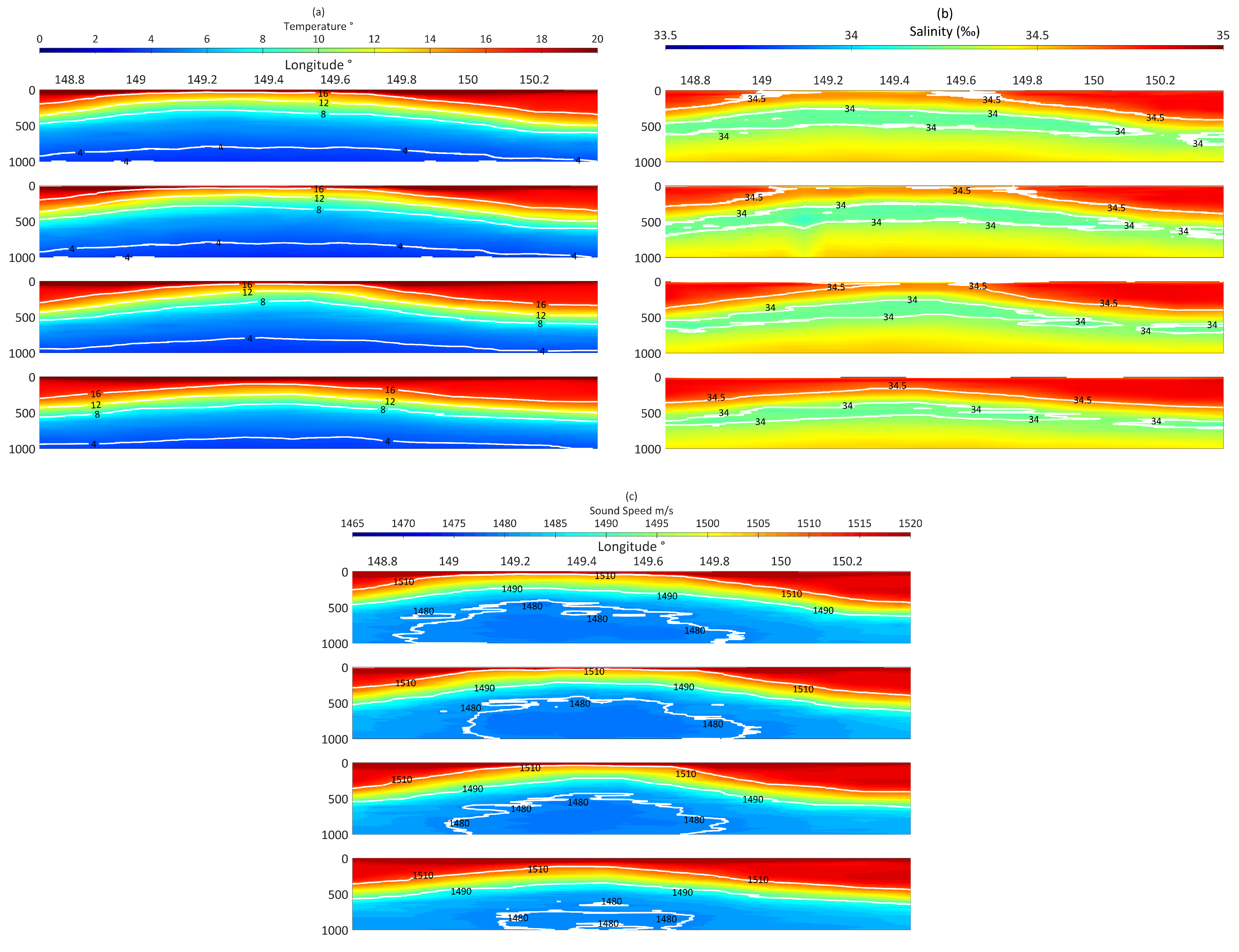
The observation data and satellite remote sensing data are used for studying the evolution process of the vertical structure, such as the growth and extinction of this cyclonic eddy. The 
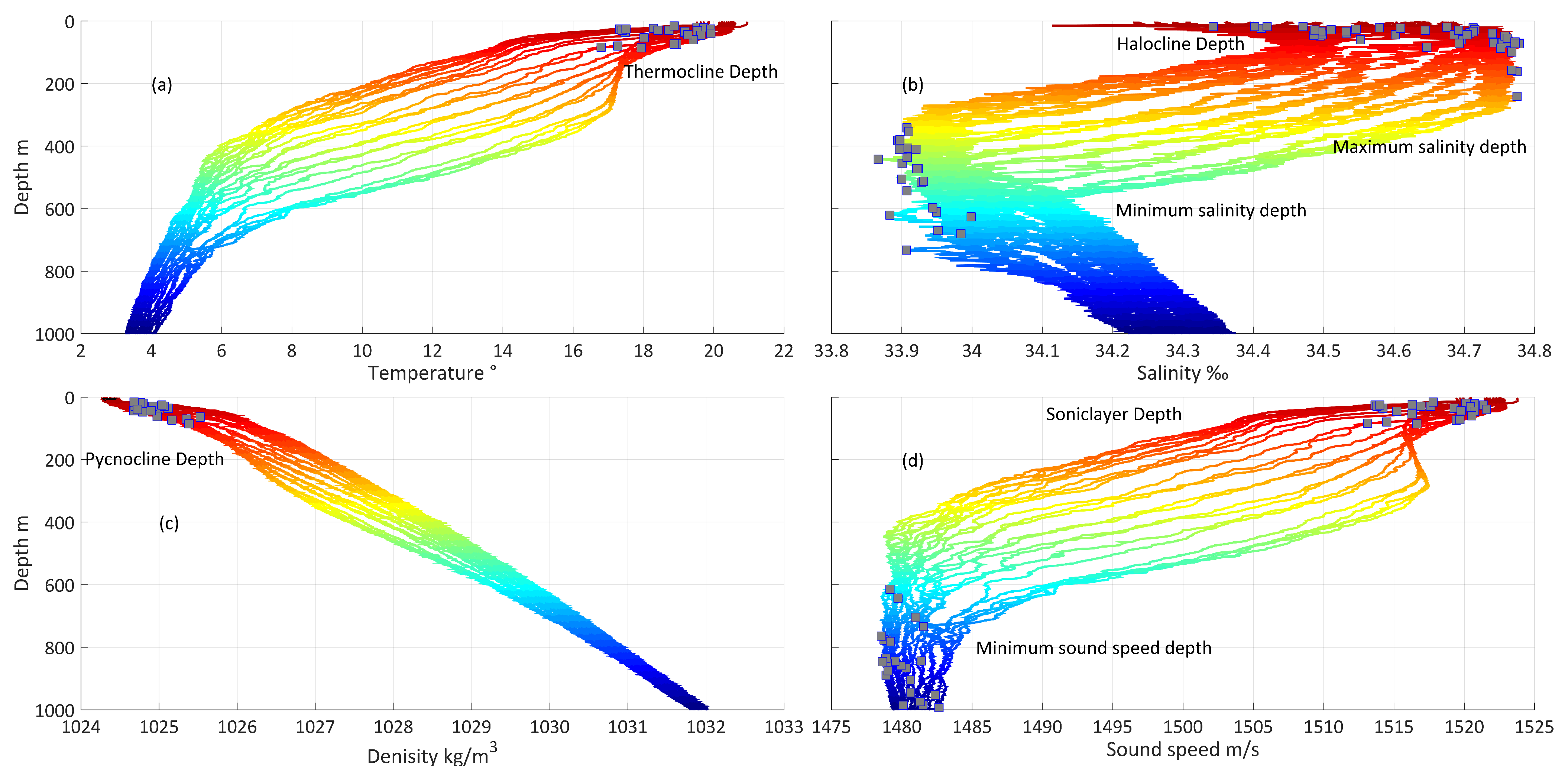
Figure 3 shows the temperature and salinity and the speed of sound profiles collected by MVP 33.7° N, 33.78° N, 33.95° N and 34.10° N, respectively. The sound propagation experiment is located at the latitude of 33.7° N section; the thermocline, halocline, sonic cline and sonic cline at each site are shown in the Figure 4.
It is known from Figure 4 that the depths of the thermocline, halocline and pycnocline came close. The position of saltation is important for human submersible vehicle and marine animal in underwater navigation and action. Above those depths, oceans mix whereby winds, turbulence and currents, the temperature, salinity, density and sound speed differ greatly. Mesoscale eddy redistributes heat and brings carbon and other elements from one part of a body of water to another. Below those depths, the temperature and sound speed gradually decreased. Taking an eddy in the North Pacific as an example, in the section of 33.7° in latitude, the depth of the maximum salinity layer (34.68 psu) is located at about 70 m, and the depth of the minimum salinity layer (33.9 psu) is about 500 m. Sound speed approximate minimum at 1480 m/s, and the depth of the sound channel is nearly 800–1000 m. Judging from Figure 3, from the surface to 300 m depth, along the latitude of the section, temperature, salinity, density and speed of sound have a peak and two valleys. The peak value position is near 149.3° E that also represents the centre of the cyclonic eddy, while the valley value locations are near 148.7° E and 150.5° E. Moreover, the difference in temperature and sound speed between the cyclonic centre and the surroundings is much weightier than that of the salinity and density. The temperature and sound speed at the eddy centre (0–1000 m vertical integral) is greater than the surrounding values by about 0.97 C and 3.5 ms 1 . While the salinity and density differences are about 0.05 psu and 0.14 kgm 3 , respectively.
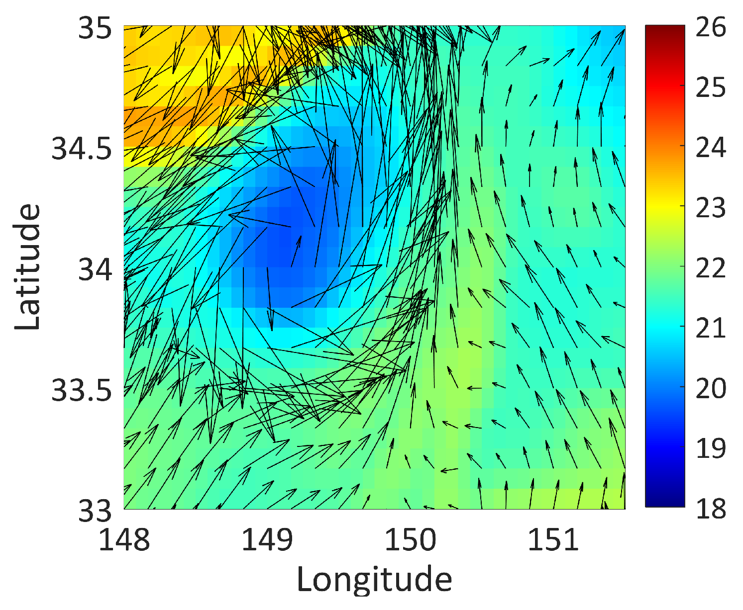
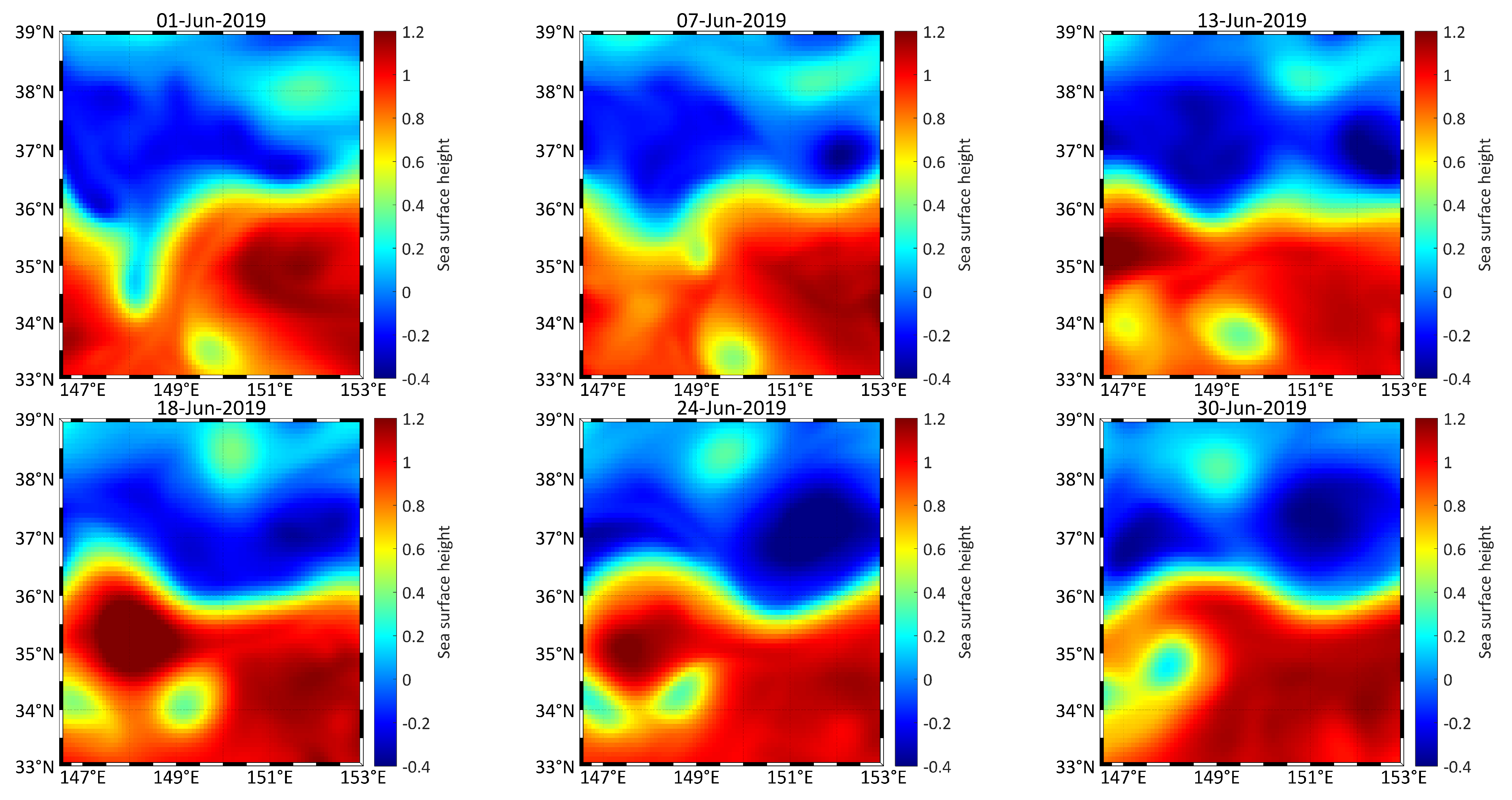
Satellite remote sensing data were obtained on the CMEMS website, and we tracked the position of the cyclonic eddy. The centre of the eddy moved westward by 18 min on the day of finishing the sound propagation experiment. The process of movement of the cyclonic was observed through sea surface height. The size, intensity and kinetic energy of the eddy increased at the early youth of the eddy’s life cycle; these characteristics remain stable in the later 3/5 of its adult period, and then rapidly decrease in the final old age of eddy’s life. As shown in Figure 5, the research area was from 148.5 to 151 east longitudes and from 33.5 to 34.5 north latitudes. The North Pacific cyclonic eddy moved westward over time and merged into Kuroshio after about three weeks. In Figure 6, the colour represents the satellite altimeters data and geostrophic velocity as the black arrow shows. Getting the information of marine and according to the sea surface temperature to determine the position of the eddy centre, we replan the acoustic propagation experiment, particularly the location of explosions. The scale of the tracked eddy is about 50 km. Combined with the distribution of hydrographic data, the eddy centre is predicted to be at 149.25° E and 34° N. 
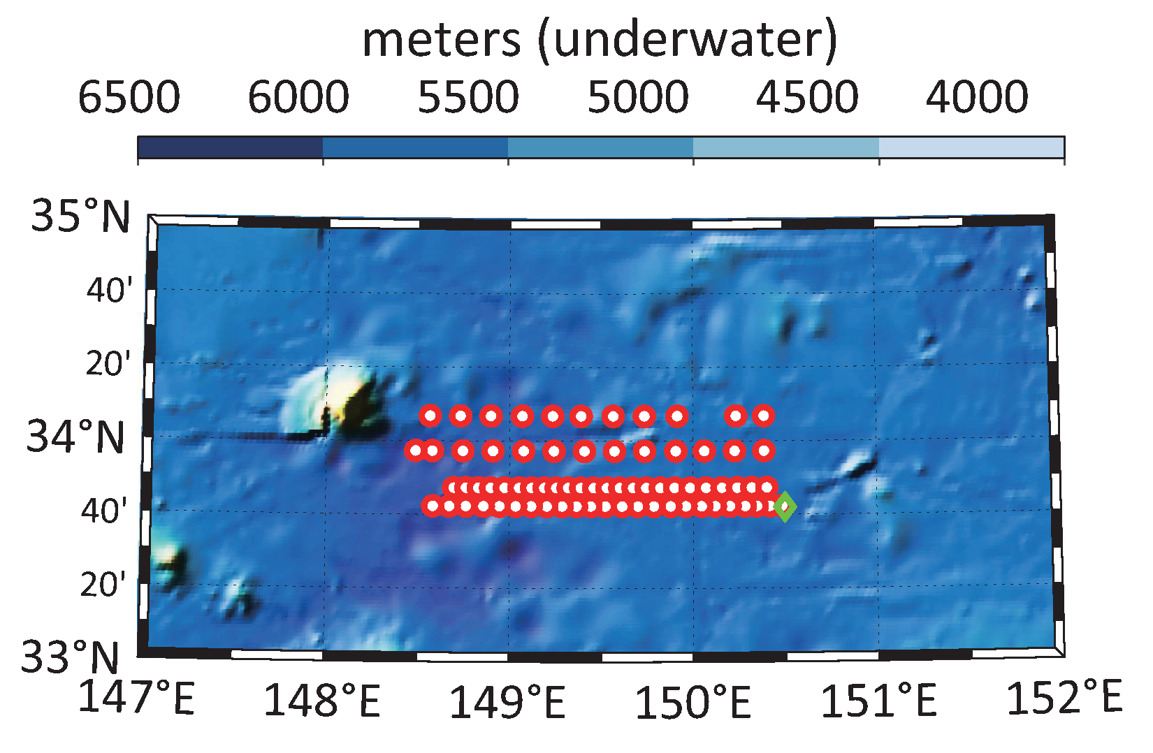
Figure 7 shows the topography of the experimental area in the western North Pacific, the path of MVP300 (red dots) and the position of the vertical line array (green circle) on 18 June 2019.

3.2. Acoustical Data

Considering multiple sources and a fixed receiver array, the acoustic reciprocity theorem was generalised. Moving explosions can be regarded as a receiver moving away from the sound source. Unfortunately, the measurement error was much higher because vertical spacing between the adjacent hydrophones is around 50 m. Only data whose standard deviation of receiver depth and hydrophones real depth are sufficiently small are selected when compared with the simulation of sound pressure transmission loss. Therefore, fewer receivers acoustic data are picked, calculated and analysed.
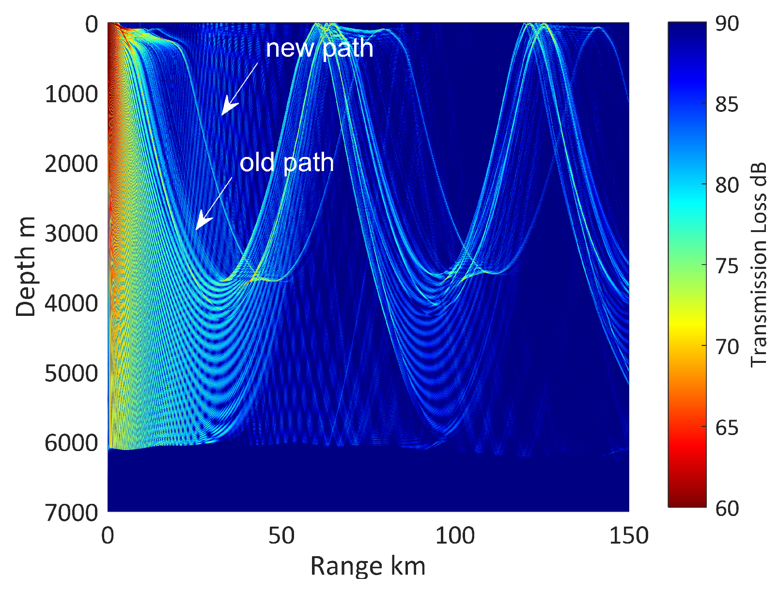
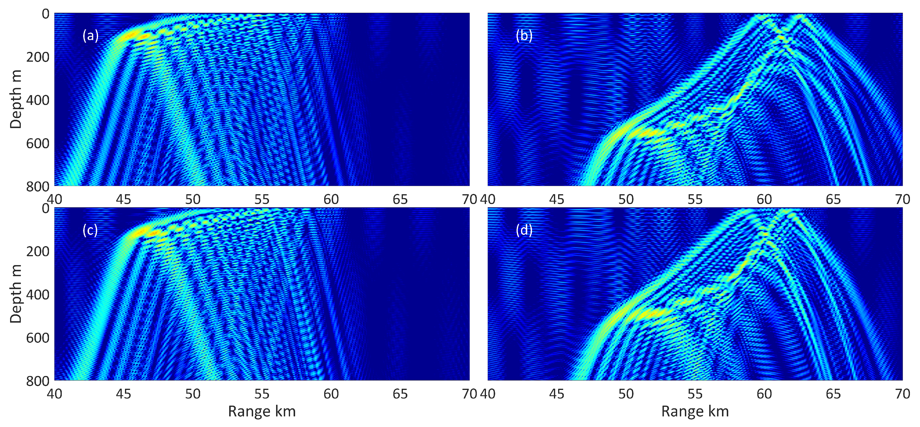
The whole depth of sound pressure transmission loss diagram is illustrated in Figure 8, and the simulated acoustic source was located in depths of 200 m. The sediment parameter is as follows: sound speed is 1650 m/s, density is 1.5 g cm 3 , and the bottom attenuation coefficient is 0.5 dB/ λ . The average depth of the ocean is 6137 m, which is approximately horizontal. Owing to the change of thermocline arising from cold-core eddy downwelling, surface sound channel (ranging from 0 m to 400 m in depth) is formed. New sound path markedly appears, as can be seen in Figure 8, marked as “new path”.
According to the eddy structure discussed in the previous section, we select the position of placing the receiver hydrophones array and the place of dropping the explosions. Through the prior simulation results of sound propagation, we know that the convergence zone was expected to be the most affected on both the energy distribution and arrival time structure. Ultimately, we dropped explosions within the scope of the first and second convergence zones, removed the locations where the ocean current has a great impact on the depth of the hydrophones, and calculated the propagation loss distribution using the remaining locations. Compared with sound pressure transmission loss impact by oceanic eddy, topography could be ignored. 
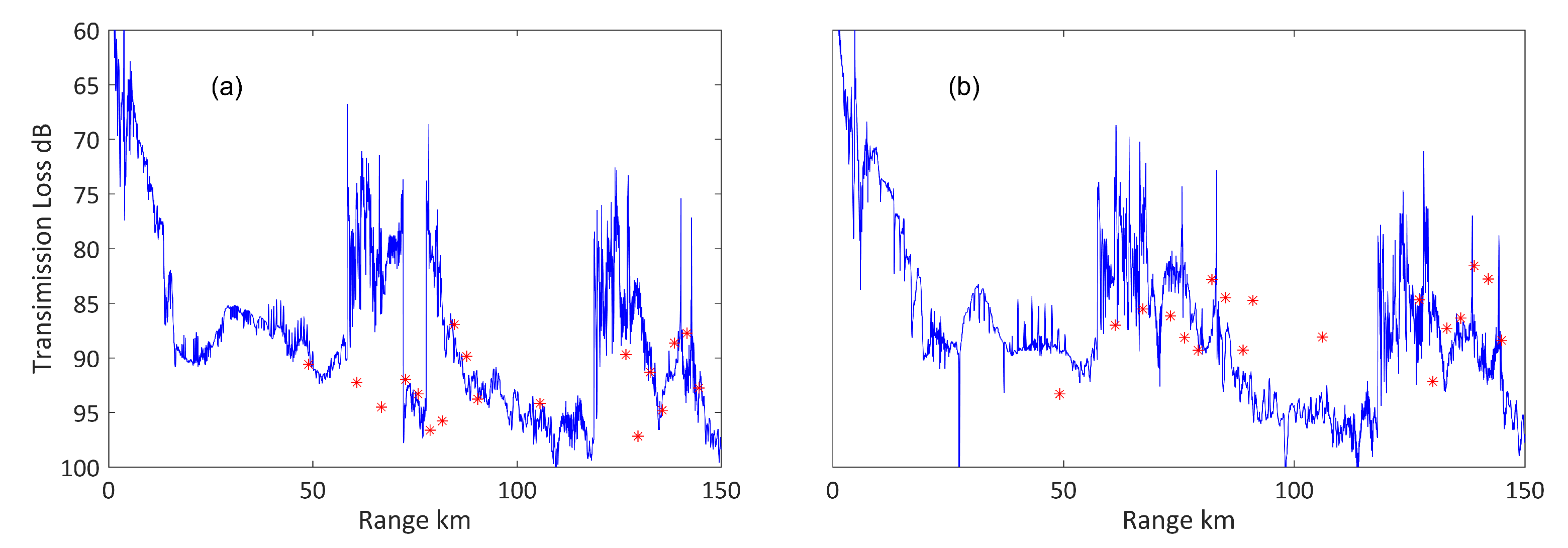
Figure 9 shows the comparison of the the numerical results with experimental data when the sound source was located in the mixed layer (200 m). The agreement of experiment and modelling can get a satisfactory result.
The curve of diagrams 
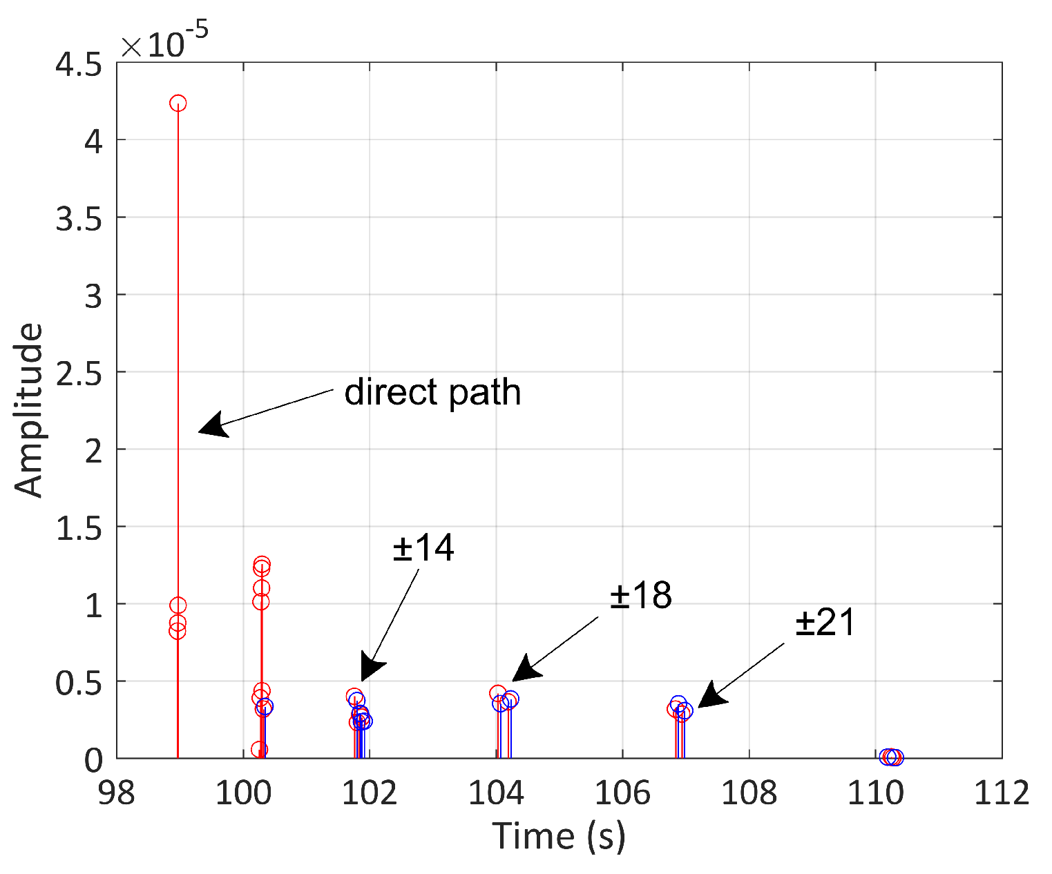
Figure 9 best illustrates the existence of a “new path”, which can be seen in the splitting of convergent zone approximately at 70 and 140 km. It is a pity that we have not been able to measure the sound propagation at the same location in the absence of the eddy situation. Eventually, the comparison of the two simulations of travel times results is given in Figure 10, which respectively are travel through the eddy and without the eddy.
For receiver at the depth of 200 m and at the range of 150 km, arrivals structure contain the number of echoes or arrivals. The direct path is missing under the circumstance of sound traversing the cyclonic eddy. An acoustic signal arrives earlier in range independent horizontal sound speed stratification environment than that of in cold-core eddy environment.

4. Discussion

4.1. Analysing the Influence of Mesoscale Eddy on the Sound Field

The analysis of effect of eddies on acoustic properties implied that the movement of the sound field converging zone is caused by the vertical gradient of the sound speed. Setting up the location of minimum sound speed profile as 1000 m, coefficient DC in Equatoin (3) is −25 m/s and 25 m/s for cyclonic and anticyclonic eddy, respectively. Furthermore, the semi-major axis of the Gaussian eddy model is 40 km, while the semi-minor axis is 400 m. Figure 11 shows sound speed contours of the cold core eddy and the warm core eddy. The bottom of the western North Pacific’s sound speed is 1650 m per second, and density is 1.5 g per cubic centimetre. The sediment parameters of deep water have little effect on the sound intensity in the distance. We select the parameters based on historical data in the Pacific. The parabolic equation method is applied to sound propagation problems to discuss how sound waves traverse eddies. The harmonic point source is located 200 m below the surface of the ocean. Subsequently, sound pressure redistribution is investigated.
A sound source produced waves of frequency 300 Hz and wavelength 5 m, and the first convergence zone typically moved 2.5 km closer to the sound source compared to that of the sound field excited in the background sound speed environment. The convergence area of the sound field influenced by the anticyclonic eddy has moved 3.3 km away from the sound source. In addition, the warm eddy has resulted in an obvious widening of the convergence zone. The sound rays go deeper into the influence region of eddies, and sound rays were no longer limited into the deep-ocean sound channel which could propagate for a great distance. As the sound rays will deflect towards a negative gradient direction of the SSP, due to the cold-core of the cyclonic eddy, more rays tend to deflect to the centre of the eddy like the convex lens effect. The rays refract gradually and deflect upwards exceeding the position where they should horizontally reverse. The width of the convergence zone became narrower, and the location of it moved toward the sea surface. Eddy intensity is characterised by the sound speed of eddy currents. Figure 12 shows the influence of intensity of eddy on transmission loss of the enlarged picture of the position of the first convergence zone. With a larger absolute intensity of the eddy, the convergence zone position moves farther away from the source. When the eddy intensity increases from 20 to 25 m/s, the sound speed changes by 1 m/s per 10 km in a horizontal direction, the location of the cyclonic eddy convergence zone moves towards the point source by 0.25 km, and the location of the anticyclonic eddy convergence zone moves away from the point source by 0.85 km.
Figure 13 shows sound propagation through cyclonic eddy and anticyclonic eddy. To analyse the affection of ocean eddy on sound transmission, typical acoustic propagation paths are drawn by white curves. Among them, SRBR is surface reflected/bottom-reflected rays, RSR is refracted/surface-reflected rays, and RR is refracted/refracted rays. SRBR rays are closely linked to seafloor parameters and are valid for short ranges (<20 km). When the ocean is deeper than the critical depth, the remainder of the depth causes the formation of a convergence zone. Except for the SRBR rays, other types of rays are influenced by the critical depth. In addition, comparing these two pictures, the change of RSR rays caused by eddies is the greatest. At the location of the first converge zone, the depth of ray reversal changes dramatically. Near the sound source, those acoustic rays have a small grazing angle corresponding to the lower-order normal mode being excited. When it comes to the position of rays convergence in Figure 13a, the sound should be reversed at a small angle; however, reversal occurs at larger angles near the sea surface and vice versa. Instead of using the ray method, analysing from the normal mode perspective can get a similar conclusion. Figure 14 illustrates, on the one hand, the whole depth function (eigenfunction) moving up at the centre of the cold eddy and, on the other hand, the whole depth function (eigenfunction ) moving down at the centre of warm eddy. Indeed, the closer the receiver position gets to the centre of the eddy, the more violently the eigenfunction moves. Above all, with the process of sound propagation, the position of the seabed reversal points moves toward the source. Then, the rays reverse near the surface more quickly, which causes the position of the convergent area to move toward the source. As a consequence, the eigenfunction at the location of the convergence zone moves both upwards and forwards. Equally, with each order eigenfunction influenced by warm-core eddy, firstly, the position of seabed reverses downwards; secondly, surface reversals occur in a position further away; thirdly, the convergence zone keeps away from the source and to the surface.

4.2. Analysing the Acoustic Characteristics of Mesoscale Eddy Using Normal Mode Method

Based on the Equation (9) in the second section, the amplitude of each order normal mode is calculated. The Figure 15 displays the normalised amplitude distribution of the normal mode of various orders at different positions away from the sound source.
The blue line illustrates the normal mode amplitude distribution under the influence of cyclonic eddy, and the red dotted line shows the normal mode amplitude distribution under the influence of anticyclonic eddy. Amplitude distribution of normal mode at various distances is calculated. At different horizontal distances, after passing through the cold eddy, that is, 100 to 200 km, the amplitude of the lower-order is generally increased. On the contrary, after passing through the warm eddy, the amplitude distribution curve of the normal mode will move towards higher-order as a whole. Affected by the eddy, the amplitude distribution of the normal mode of each order varies greatly from 10 to 90 km away from the source. Under the influence of the cold eddy, when the receiver position moves from the eddy edge to the position close to the eddy centre, more energy is distributed in the higher-order, corresponding to more sound rays emitted from the source at a larger grazing angle. Those rays have a shorter sound path, and a nearby convergence zone occurs at a close distance. However, under the influence of the warm eddy, when the receiver position moves from the edge of the eddy to the position close to the eddy centre, more energy is distributed in the lower order, corresponding to more sound rays emitted from a comparatively smaller grazing angle. These rays have longer sound paths, and energy will converge at a greater distance.
Figure 16 shows the coupling matrix at 10, 50 and 90 km of the main orders of normal mode. The left panel is the distribution of the coupling coefficient affected by the cyclonic eddy, and the right panel is the distribution of the coupling coefficient affected by the anticyclonic eddy. Because the eddy centre is located above the background sound channel axis, sound speed continues to decrease at 500 m below sea level, causing the change of the depth of the axis of the sound channel. For the cold-core eddy, the order of the normal mode coupling is more than that of the warm-core eddy. In addition, the reasons for the variation of the coupling strength of the normal mode at different distances from the eddy center can be influenced by the variation rate of sound speed.
Measurement of sound speed of the eddy is used for taking everything into account. From Figure 17 we can learn that, with the movement of the distance to the centre of the eddy, normal mode theory is used for getting the amplitude of local modes at different distances to the centre of the eddy. The same as the simulation of the cold eddy, the measured eddy shows the same conclusion that the amplitude of higher-order normal modes increases when the receiver position is to the centre of the eddy.

5. Conclusions

Mesoscale eddy will lead to changes in the location of the convergence zone relative to the acoustic source position. The convergence zone shifts toward the acoustic source as the cyclonic eddy occurs on the acoustic propagation path, and the anticyclonic eddy causes the convergence zone to move away from the acoustic source and increases the width of the convergence zone. Each order eigenfunction moves up influenced by cold-core eddy (moves down influenced by warm-core eddy); the seabed reversal points move toward (away from) the source, and then, the rays reverse near the surface moves toward (away from) the source. The eddy causes the amplitude of normal modes to be different at different positions away from the source. For the cyclonic eddy, the amplitude of higher-order normal modes increases when the receiver is close to the centre of the eddy; on the contrary, the amplitude of lower-order normal modes increases when the receiver is close to the centre of the anticyclonic eddy. We researched both source and receiver near the sea surface sound propagation problem with the effect of eddies. It brought with it a clarity of purpose, an easy understanding of human submersible vehicles and large marine creatures. They are known to produce low-frequency sounds that can propagate over long distances and receive echoes, detect underwater objects and locate food. Eddies could interfere with them in their prediction of distance and range.

Author Contributions

Conceptualization, S.P.; methodology, J.L. and S.P.; software, J.L. and Y.G.; validation, J.L.; formal analysis, J.L., S.P. and Y.G.; investigation, J.L., L.G. and M.Z.; resources, S.P.; writing—original draft preparation, J.L. and L.G.; writing—review and editing, J.L., S.P., L.G., M.Z., Y.G. and S.Z.; visualization, S.P. and L.G.; supervision, S.P.; project administration, S.P.; funding acquisition, S.P. All authors have read and agreed to the published version of the manuscript.

Funding

This research was funded by National Natural Science Foundation of China, grant number 11904065.

Acknowledgments

The measuring of oceanic front data of the north-western ocean and the experiments of acoustic propagation were accomplished with the help of College of Meteorology and Oceanography in National University of Defense Technology.

Conflicts of Interest

The authors declare no conflict of interest.

References

  1. Lochte, K.; Pfannkuche, O. Cyclonic cold-core eddy in the eastern North Atlantic. II. Nutrients, phytoplankton and bacterioplankton. Mar. Ecol. Prog. Ser. 1987, 39, 153–164. [Google Scholar] [CrossRef]
  2. National Research Council. Marine Mammals and Low-Frequency Sound: Progress Since 1994; National Academies Press: Washington, DC, USA, 2000. [Google Scholar]
  3. Godø, O.R.; Samuelsen, A.; Macaulay, G.J.; Patel, R.; Hjøllo, S.S.; Horne, J.; Kaartvedt, S.; Johannessen, J.A. Mesoscale eddies are oases for higher trophic marine life. PLoS ONE 2012, 7, e30161. [Google Scholar] [CrossRef] [PubMed] [Green Version]
  4. Tyack, P. Acoustic communication under the sea. In Animal Acoustic Communication; Springer: Berlin/Heidelberg, Germany, 1998; pp. 163–220. [Google Scholar]
  5. Waite, A.M.; Raes, E.; Beckley, L.E.; Thompson, P.A.; Griffin, D.; Saunders, M.; Säwström, C.; O’Rorke, R.; Wang, M.; Landrum, J.P.; et al. warm-core eddies: Implications for the zooplankton isoscape and rock lobster larvae. Limnol. Oceanogr. 2019, 64, 2405–2423. [Google Scholar] [CrossRef]
  6. Kobashi, F.; Kawamura, H. Seasonal variation and instability nature of the North Pacific Subtropical Countercurrent and the Hawaiian Lee Countercurrent. J. Geophys. Res. Ocean. 2002, 107, 6-1–6-18. [Google Scholar] [CrossRef]
  7. Goh, G.; Noh, Y. Influence of the Coriolis force on the formation of a seasonal thermocline. Ocean Dyn. 2013, 63, 1083–1092. [Google Scholar] [CrossRef]
  8. Lin, X.; Dong, C.; Chen, D.; Liu, Y.; Yang, J.; Zou, B.; Guan, Y. Three-dimensional properties of mesoscale eddies in the South China Sea based on eddy-resolving model output. Deep Sea Res. Part I Oceanogr. Res. Pap. 2015, 99, 46–64. [Google Scholar] [CrossRef]
  9. Henrick, R.; Jacobson, M.; Siegmann, W.; Clark, J. Use of analytical modeling and limited data for prediction of mesoscale eddy properties. J. Phys. Oceanogr. 1979, 9, 65–78. [Google Scholar] [CrossRef] [Green Version]
  10. Dong, C.; Mavor, T.; Nencioli, F.; Jiang, S.; Uchiyama, Y.; McWilliams, J.C.; Dickey, T.; Ondrusek, M.; Zhang, H.; Clark, D.K. An oceanic cyclonic eddy on the lee side of Lanai Island, Hawai’i. J. Geophys. Res. Ocean. 2009, 114. [Google Scholar] [CrossRef] [Green Version]
  11. Jensen, F.B.; Kuperman, W.A.; Porter, M.B.; Schmidt, H. Computational Ocean Acoustics; Springer Science & Business Media: Berlin/Heidelberg, Germany, 2011. [Google Scholar]
  12. Jian, Y.; Zhang, J.; Liu, Q.; Wang, Y. Effect of mesoscale eddies on underwater sound propagation. Appl. Acoust. 2009, 70, 432–440. [Google Scholar] [CrossRef]
  13. Nysen, P.A.; Scully-Power, P.; Browning, D.G.; Bannister, R.W. Project ANZUS Eddy: Acoustic measurement of a warm core ocean eddy. J. Acoust. Soc. Am. 1975, 58, S31. [Google Scholar] [CrossRef]
  14. Nysen, P.A.; Scully-Power, P.; Browning, D.G. Sound propagation through an East Australian Current eddy. J. Acoust. Soc. Am. 1978, 63, 1381–1388. [Google Scholar] [CrossRef]
  15. Lawrence, M.W. Modeling of acoustic propagation across warm-core eddies. J. Acoust. Soc. Am. 1983, 73, 474–485. [Google Scholar] [CrossRef]
  16. Baer, R.N. Calculations of sound propagation through an eddy. J. Acoust. Soc. Am. 1980, 67, 1180–1185. [Google Scholar] [CrossRef]
  17. Weinberg, N.; Clark, J. Horizontal acoustic refraction through ocean mesoscale eddies and fronts. J. Acoust. Soc. Am. 1980, 68, 703–705. [Google Scholar] [CrossRef]
  18. Heaney, K.D.; Campbell, R.L. Three-dimensional parabolic equation modeling of mesoscale eddy deflection. J. Acoust. Soc. Am. 2016, 139, 918–926. [Google Scholar] [CrossRef] [PubMed]
  19. Dozier, L.; Tappert, F. Statistics of normal mode amplitudes in a random ocean. I. Theory. J. Acoust. Soc. Am. 1978, 63, 353–365. [Google Scholar] [CrossRef]
  20. Colosi, J.A.; Morozov, A.K. Statistics of normal mode amplitudes in an ocean with random sound-speed perturbations: Cross-mode coherence and mean intensity. J. Acoust. Soc. Am. 2009, 126, 1026–1035. [Google Scholar] [CrossRef] [Green Version]
  21. Spall, M.A. Dynamics of downwelling in an eddy-resolving convective basin. J. Phys. Oceanogr. 2010, 40, 2341–2347. [Google Scholar] [CrossRef] [Green Version]
  22. Calado, L.; Gangopadhyay, A.; Da Silveira, I. A parametric model for the Brazil Current meanders and eddies off southeastern Brazil. Geophys. Res. Lett. 2006, 33. [Google Scholar] [CrossRef] [Green Version]
  23. Collins, M.D. Applications and time-domain solution of higher-order parabolic equations in underwater acoustics. J. Acoust. Soc. Am. 1989, 86, 1097–1102. [Google Scholar] [CrossRef]
  24. Tappert, F. Parabolic equation method in underwater acoustics. J. Acoust. Soc. Am. 1974, 55, S34. [Google Scholar] [CrossRef]
  25. Tappert, F.D. The parabolic approximation method. In Wave Propagation and Underwater Acoustics; Springer: Berlin/Heidelberg, Germany, 1977; pp. 224–287. [Google Scholar]
  26. Pierce, A.D. Extension of the method of normal modes to sound propagation in an almost-stratified medium. J. Acoust. Soc. Am. 1965, 37, 19–27. [Google Scholar] [CrossRef]
Figure 1. (a) Cyclonic eddy and (b) anticyclonic eddy three-dimensional schematic diagram. Shades of colour represent the water column temperature level, the red part has the highest temperature; by contrast the blue part has the lowest temperature, and the red arrow represents the direction of the eddy current in the northern hemisphere.
Jmse 09 00787 g001
Figure 2. Sound propagation experiment configuration.
Jmse 09 00787 g002
Figure 3. Measured data of (a) temperature, (b) salinity and (c) sound speed and each sub-figure from top to bottom was located at the latitude of 33.7°, 33.78°, 33.95° and 34.10° E.
Jmse 09 00787 g003
Figure 4. Measured data at the latitude of 33.7° N, (a) temperature, (b) salinity, (c) density and (d) sound speed profiles.
Jmse 09 00787 g004
Figure 5. Sea surface height of the life cycle of the eddy.
Jmse 09 00787 g005
Figure 6. Sea surface temperature and geostrophic velocity of the eddy.
Jmse 09 00787 g006
Figure 7. Topography of the western North Pacific. Colour shading indicates topographic relief from etopo1 data.
Jmse 09 00787 g007
Figure 8. Sound transmission loss propagation through the eddy.
Jmse 09 00787 g008
Figure 9. Transmission loss and experimental results in depths of 200 m (red asterisk), 100 m explosions (a) and 200 m explosions (b), and the blue line is simulated sound pressure transmission loss with a different range.
Jmse 09 00787 g009
Figure 10. Arrivals in blue travel through the eddy and in red is travel without the eddy. The arrow points out sound exit angle from the source.
Jmse 09 00787 g010
Figure 11. Sound speed distribution of cyclonic eddy (a) and anticyclonic eddy (b).
Jmse 09 00787 g011
Figure 12. Transmission loss of convergence zone 25 m/s intensity of cyclonic eddy (a) and anticyclonic eddy (b) and 20 m/s intensity of cyclonic eddy (c) and anticyclonic eddy (d).
Jmse 09 00787 g012
Figure 13. Transmission loss distribution of cyclonic eddy (a) and anticyclonic eddy (b).
Jmse 09 00787 g013
Figure 14. The eigenfunctions vary with depth influenced by eddy; red line represents warm-core eddy, and blue line represents cold-core eddy. (a) 40 km away from the center of eddy; (b) 0 km away from the center of eddy.
Jmse 09 00787 g014
Figure 15. Normalised amplitude distribution of normal mode at different distances from the sound source, which are (a) 10 km, (b) 50 km, (c) 90 km and (d) 150 km away from the source.
Jmse 09 00787 g015
Figure 16. Coupling coefficient affected by cold eddy: (a) 10 km, (b) 50 km and (c) 90 km away from the source and coupling coefficient effected by warm eddy (d) 10 km, (e) 50 km and (f) 90 km away from the source.
Jmse 09 00787 g016
Figure 17. Normalised amplitude distribution of normal mode affected by real eddy at different positions from the sound source, which are (a) 10 km, (b) 50 km, (c) 90 km and (d) 150 km away from the source.
Jmse 09 00787 g017
Publisher’s Note: MDPI stays neutral with regard to jurisdictional claims in published maps and institutional affiliations.

