A General-Purpose Biotic Index to Measure Changes in Benthic Habitat Quality across Several Pressure Gradients

Abstract

Realistic assessments of the ecological status of benthic habitats, as requested by European directives such as the Water Framework Directive and the European Marine Strategy Framework Directive, require biotic indices capable of detecting anthropogenic impact without having preliminary knowledge of the occurring pressures. In this context, a new general-purpose biotic index (GPBI) based on the deviation of benthic macrofauna community composition and structure from a valid reference (i.e., good ecological status) is proposed. GPBI is based on the assumption that as a site becomes impacted by a pressure, the most sensitive species are the first to disappear, and that stronger impacts lead to more important losses. Thus, it explicitly uses the within-species loss of individuals in the tested station in comparison to one or several reference stations as the basis of ecological status assessment. In this study, GPBI is successfully used in four case studies considering the impact of diversified pressures on benthic fauna: (1) maerl extraction in the northern Bay of Biscay, (2–3) dredging and trawling in the North Sea, and (4) hypoxic events at the seafloor in the Gullmarfjord. Our results show that GPBI was able to efficiently detect the impact of the different physical disturbances as well as that of hypoxia and that it performs better than commonly used pressure-specific indices (M-AMBI and TDI). Signal detection theory was used to propose a sound good/moderate ecological quality status boundary, and recommendations for future monitoring are also provided based on the reported performance of GPBI.

1. Introduction

The Water Framework Directive (WFD, 2000/60/EC, European Commission, 2000) and the European Marine Strategy Framework Directive (MSFD, 2008/56/EC, European Commission, 2008) have boosted scientific research devoted to the assessment of the ecological quality status (EcoQ) of marine habitats [1]. The use of benthic macrofauna to assess EcoQ has proven to be highly valuable, and this has led to the development of several benthic biotic indices. Diaz et al. [2] reviewed 64 such biotic indices, 33 of which were based only on macrofauna. It is their considerable stability in space and time and thus their capacity to integrate pressure impacts over long timescales that make benthic communities particularly suited for long-term investigations and quality assessments [2,3,4].

The EU Water Framework Directive (WFD) was established in 2000, and indices such as the biotic index of Grall and Glémarec [5], the AZTI Marine Biotic Index (AMBI, [6,7]), and the multivariate AMBI (M-AMBI, [8]) were developed for the purpose of assessing coastal waters (<1 Nm), which are particularly subject to organic enrichment and eutrophication. Although they have been used to detect a wide variety of anthropogenic disturbances, the assignment of species to sensitivity groups is in general related to an organic enrichment pressure [5,6,9,10] and based on the seminal work of Pearson and Rosenberg [3]. Later, the MSFD extended these objectives and aimed at reaching good environmental status in both coastal and open-sea waters (down to the bathyal zone). The benthic habitats to be evaluated spread over large extents of the continental shelf where bottom trawling and dredging replace organic enrichment and eutrophication as the most common anthropogenic disturbances [11,12]. The impact of such direct physical disturbances on benthic communities is not always detected with AMBI and M-AMBI, as these indices were designed for organic enrichment [13,14]. Nevertheless, environmental managers need simple indices to assess EcoQ on the continental shelf, and these indices are still relied upon. In the case of the assessment of EcoQ on the continental shelf, the trawling disturbance index (TDI, [15]) and TDI-derived indices such as modified TDI (mTDI, [16]), partial TDI (pTDI), and the modified vulnerability index (mT, modified from [17]) have proved to vary with fishing effort [15,18]. These indices were developed to assess trawling pressure and consider species biological traits relevant to this type of pressure. Both M-AMBI and TDI are based on a classification of taxa on a scale of sensitivity/tolerance to a defined pressure (organic and physical, respectively) according to literature data and/or expert judgment.

Apart from their ease of use, indices based on classification of taxa present several weaknesses: (1) the list of species must be extremely large in order to use them in different habitats, regions, and seas; (2) literature concerning the sensitivity of species is not exhaustive; (3) they are not usable with any type of pressure; and (4) we often make mistakes in linking the abundance and the sensitivity species lists because of change in names of species, spelling mistakes, or omissions in the correspondence between species names and sensitivity groups/traits attributed to higher taxonomic levels. Indices based on the deviation of community composition between reference stations and tested stations constitute an interesting alternative to these problems [19,20]. Flåten et al. [19] proposed a community disturbance index (CDI) based on the ratio between the residual of fauna composition at the tested station and the expected reference community, as modeled from observational data at undisturbed reference stations. Along the same line, Johnson et al. [20] proposed a simpler approach for detecting potential disturbances based on the comparison of benthic fauna composition at a tested station with the composition at a reference station using the Bray-Curtis similarity index.

Approaches based on the deviation of faunal composition from a reference stage have the advantage that they are potentially able to detect any kind of pressure effects inducing changes in benthic macrofauna community composition or structure (i.e., the very first hypothesis underlying the development of benthic biotic indices). Nevertheless, the spatial and temporal distribution of organisms is influenced by a variety of natural factors [20] interfering with the relationship of the intensity of pressure and its biological effects [21]. Furthermore, a potential pitfall of using Bray-Curtis similarity as an indicator of deviation from the reference state is the lack of univocal direction of the relationship linking pressure intensity changes to deviation measures. In other words, the increase in abundance of certain species can lead to dissimilarities that are not necessarily associated with a degradation of the ecosystem, especially when no species decrease in abundance or disappear. This may explain why none of the above-mentioned approaches resulted in further testing and/or applications.

A potential way forward is to focus on the within-species loss of individuals between the reference station and the tested station. This is supported by the rationale that species sensitive to a given pressure will tend to decrease in abundance and eventually disappear. The proportion of lost individuals for a given species will tend to increase with increasing disturbance, and this should be linked to a decrease in EcoQ. Even though peaks of opportunists may appear simultaneously, sensitive species will continue to decrease in abundance. Consequently, sensitivity grouping or functional trait matrices are not necessary as the first species with decreasing abundances are considered to be the most sensitive ones to the pressure. Therefore, a biotic index based on this proportion should (1) be able to detect any kind of disturbance and (2) be independent of any preclassified list of sensitivity/tolerance, which potentially allows for its application in any kind of area and for any kind of disturbance/habitat relationship.

In this context, we here propose the general-purpose biotic index (GPBI) based on the assumption that a pressure has an impact on the environment as soon as the most sensitive species suffer a reduction in their abundance. The objectives of the present study are to (1) develop a new biotic index for assessing the EcoQ of benthic habitats based on the deviation of benthic macrofauna composition and structure as compared to a valid reference, (2) test the response of this index to known and quantified disturbances through a meta-analysis of four case studies, (3) compare its performance with two other commonly used indices: M-AMBI (because it is widely used, in all types of disturbance contexts) and TDI (because it may be a good candidate to assess EcoQ on continental shelves), and (4) provide first insights on the setting of threshold values of this index to classify EcoQ. Recommendations for the sampling design and data analysis procedures to be implemented as part of future monitoring using this index are also provided.

2. Materials and Methods

2.1. Computation of the GPBI

The first component of the proposed new biotic index (GPBI) is a measure of loss in comparison to a reference station. For a tested station (t), we first compute the proportion (R_quant) of species abundances at the reference station (r) that is absent from the tested station:

$$R_{quant\left\{r;t\right\}}=1-\frac{{\sum }_{i=1}^{S_r }max\left(r_i-t_i;0\right)}{{\sum }_{i=1}^{S_r}{r}_i}$$

(1)

where S_r is the species richness at the reference station, r_i is the abundance of species i at the reference station, and t_i is the abundance of species i at the tested station. This proportion is in fact the complement of the quantitative generalization of the binary similarity coefficient proposed by Ruggiero et al. [22] that measures the proportion of species present at the reference station that are also found at the tested station (hence the name R_quant). Koleff et al. [23] re-expressed the index of Ruggiero et al. [22] as a/(a+c), where c is the number of species present at the reference station and a is the number of species present at both the reference and tested station. Likewise, we can define A as the sum of species abundances common to both sites and C as the sum of species abundances exclusive to the reference station [24]. We can then simply define R_quant for a tested station as follows:

$$R_{quant\left\{r;t\right\}}=\frac{A}{A+C} or equivalently R_{quant\left\{r;t\right\}}=1-\frac{C}{A+C}$$

(2)

If there is a single reference station, then the index for tested station t ($GPB{I}_{\left\{t\right\}}$) is computed as follows:

$$GPB{I}_{\left\{t\right\}}=R_{quant\left\{r;t\right\}}$$

(3)

If there are multiple reference stations, $GPB{I}_{\left\{t\right\}}$ is computed as follows:

$$GPB{I}_{\left\{t\right\}}=1-\left|\overline{ref}-\%loss\right|$$

(4)

where $\%loss$ is the average of the $R_{quant\left\{r;t\right\}}$ for station t in comparison to each reference station and $ref$ is the average of all values in the R_quant similarity matrix between reference stations, including its diagonal. This allows for accounting for variability among good-quality stations and the a priori set of reference stations, as well as detecting degradation in tested stations where %loss is expected to increase with loss of quality.

Equations (3) and (4) both give an index ranging from 0 (bad EcoQ) to 1 (good EcoQ).

An available R function (Supplementary Material S1) with data and examples on how to use the code (Supplementary Material S2, S3) is offered.

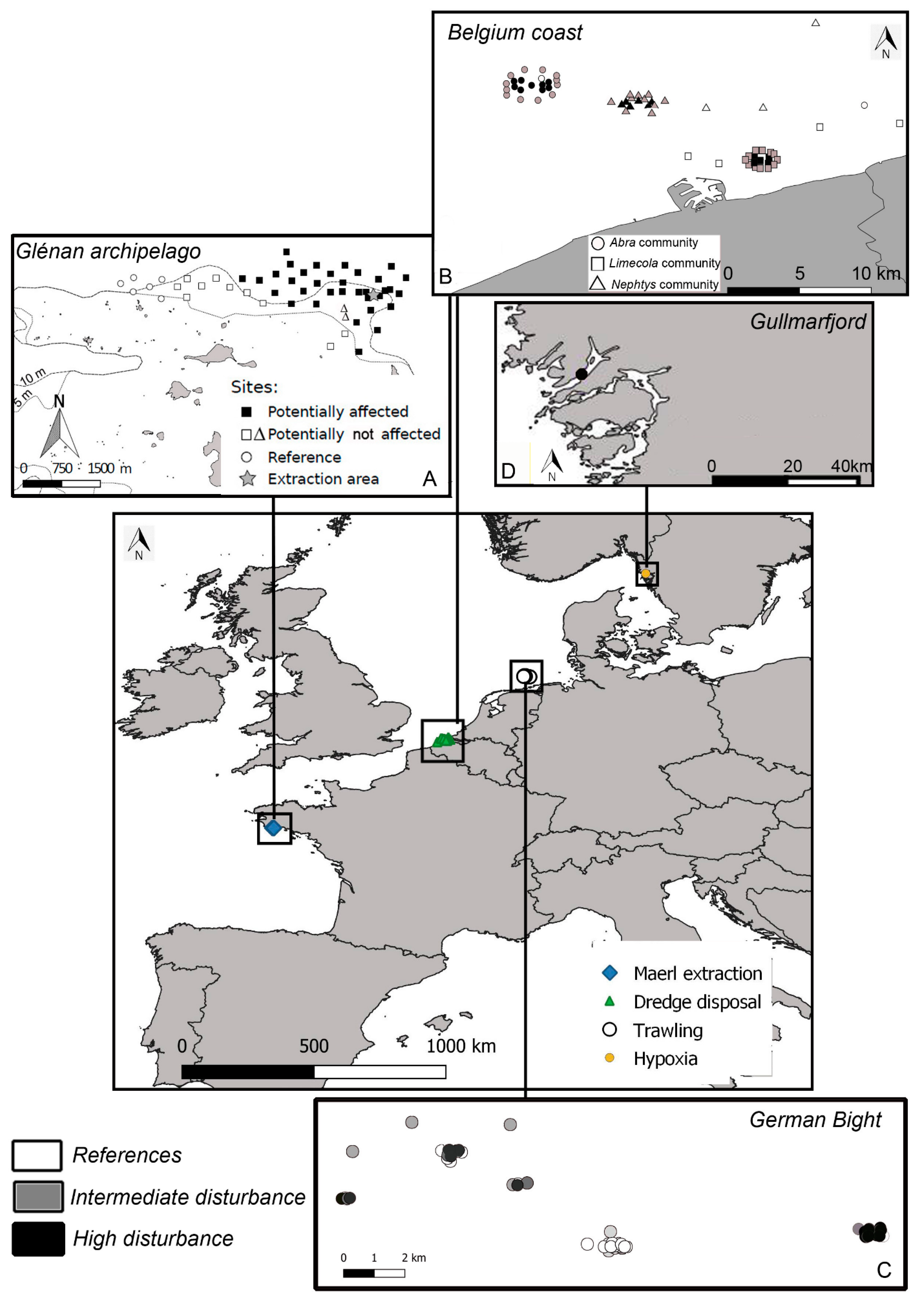
2.2. The Four Case Studies

Four case studies are used to illustrate the proposed index, each one exemplifying the impact of one particular kind of pressure acting on benthic habitats and potentially affecting benthic macrofauna communities. Importantly, corresponding data sets all included benthic macrofauna samples taken across a pressure gradient, together with a quantitative parallel assessment of the level of the given pressure. The ability (performance) of the new biotic index (GPBI) to describe changes in pressure level was assessed for each data set and compared to the performance of widely used indices such as M-AMBI and TDI. Translation of the GPBI values into EcoQ was finally performed on the basis of signal detection theory [25].

2.2.1. Case Study 1: Maerl Extraction (France, Bay of Biscay)

Glénan Archipelago is located in the northern Bay of Biscay. Maerl beds refer to free-living coralline algae (Corallinophycidae, Rhodophyta) accumulating on soft sediment to form highly structured and productive biogenic benthic habitats. The Glénan maerl bed is one of the largest (4.5 km²) and thickest (up to 16 m) in Brittany. It has been industrially exploited from 1970 to 2011, which generated a gradient of physical pressure over 100 hectares. Maerl extraction causes direct habitat loss with severe impacts on associated biota [26]. Moreover, after extraction, maerl is washed at sea, inducing the release of large quantities of fine particles that sink back onto the seabed. This can cause maerl mortality and alter maerl-associated biota over a much wider spatial scale than the extraction area [27]. A total of 52 stations were sampled in April 2003 for benthic community analysis (Figure 1). Three 0.1 m² Van Veen grab samples were collected at each station and sieved on a 1 mm mesh size. Each of them was heavily loaded (i.e., from 10 to 15 L each). Back at the laboratory, benthic macrofauna was sorted and identified down to the species level. Sampled stations were a priori classified in three groups: (1) “reference” (most unlikely to be affected), (2) “potentially not affected” and (3) “potentially affected” based on the Telemac-2D hydro-sedimentary model, which takes into account maerl extraction location, timing, volumes, and tide currents [28]. Potentially affected stations were defined as those with more than 1 mg L⁻¹ of inorganic suspended matter above natural conditions. Of the remaining stations, those in close proximity to the extraction point were classified as potentially affected due to the uncertainty of the model. All remaining stations were classified as reference. Data used for this case study are available in Supplementary Material S2.

2.2.2. Case Study 2: Dredge Disposal Pressure (Belgium, North Sea)

This case study considers five dredge disposal dumping sites in the coastal area of the Belgian part of the North Sea [29]. These are located in three habitat types, namely the Abra alba community (noncohesive muddy fine sand dominated by the bivalves Abra alba and Nucula nitidosa, ampeliscid amphipods, and polychaetes), the Limecola balthica community (shallow infralittoral mud dominated by the bivalves Limecola balthica and Nucula nitidosa, the polychaetes Nephtys hombergii and Lagis Koreni, and the sand-dwelling urchin Echinocardium chordatum), and the Nephtys cirrosa community (well-sorted relatively mobile medium/fine sands dominated by the polychaetes Nephtys cirrosa and Magelona mirabilis and the amphipods Bathyporeia spp. and Pontocrates spp.), as defined by Breine et al. [30]. The sites were sampled following a control–impact design, with a set of samples within the designated site and a set of control samples outside the site. The samples were taken with a Van Veen grab (0.1 m²) and sieved on 1 mm mesh size and fixed in 8% buffered formalin. Sampled specimens were identified to the lowest possible taxonomic level. The value of pressure reported for each station corresponds to the amount of material disposed the year preceding sampling. On each sampling occasion, 3 levels of pressure were considered: (1) no dredging (considered as reference), (2) an intermediate volume dredged (stations were submitted to 40,000 tonnes dry matter in the three communities for all sampling occasions), and (3) a high volume dredged (varying between 3,587,117 and 6,265,121 tonnes dry matter for the Abra community, between 2,944,509 and 4,667,225 tonnes dry matter for the Limecola community, and between 80,014 and 3,003,096 tonnes dry matter for the Nephtys community).

2.2.3. Case Study 3: Trawling Pressure (Germany, North Sea)

The study site is situated in the German Bight (North Sea) 30 nm off the island of Borkum at 30 m water depth. The sediment consists of homogenous fine sands. In this area, a research platform was built as a pilot project for future offshore wind farms in July 2003. The area surrounding the platform (500 m radius) is closed to all shipping activities (except scientific activities) and is thus protected from fisheries (for further details, see [31]). To estimate the impact of trawling in the study area, trawling intensity was calculated by means of the satellite-based “Vessel Monitoring System” for the main operating fleets (VMS data for Dutch and German fleets; unpublished data provided by S. Ehrich, Federal Research Centre for Fisheries, and by G. Piet and F. Quirins, Netherlands Institute for Fisheries Research). Swept area ratio (SAR) indicative of trawling intensity was calculated as times trawled month⁻¹ (i.e., × spot⁻¹) following the two-step procedure of Rijnsdorp et al. [32]:

The spatial distribution of the fleet was raised to the fishing effort of the total fleet in hours fished per month. The trawling frequency per area (F) was calculated according to

$$F_i=\frac{R_i\times \left(T_j÷N_j\right)}{H}$$

(5)

where R_i corresponds to the trawling hours from VMS records in unit i, T_j is the total number of fishing hours of the total fleet in ICES rectangle j, N_j is the number of fishing hours of the sampled fleet in ICES rectangle j, and H is the number hours corresponding to a beam trawl intensity of once every year.

The number of hours corresponding to a beam trawl intensity of once per year (H) was calculated from the surface area trawled per hour and the surface area of the spatial unit fished (1° latitude × 2° longitude). The whole procedure was repeated separately for large (>300 hp) and small (≤300 hp) vessels.

For the larger beam trawlers (2 × 12 m beam trawl width) an average fishing speed of 7 knots was assumed. Thus, one fishing hour corresponds to a surface area trawled of 0.311 km². At 54° N, the surface area of a unit of 1° latitude × 2° longitude equals 1.852 × 2 × 1.852 × cos(latitude) = 4.032 km². Consequently, for large beam trawlers, H = 4.032/0.311 = 12.96 h.

For the smaller beam trawlers (2 × 12 m beam trawl width) an average fishing speed of 5 knots was assumed. Thus, one fishing hour corresponds to a surface area trawled of 0.130 km². Consequently, for small beam trawlers, H = 4.032/0.130 = 31.10 h. Trawling intensity was calculated from VMS records for the years 2003–2004.

There were no spatial trends or differences in trawling intensity detectable between the study sites prior to closure; i.e., seasonality is the major determinant of trawling intensity (see Figure 2 in [33]). An “unfished area” was defined between an inner circle of 150 m radius (to avoid platform effects) and an outer circle of 400 m radius (to avoid trawling edge effects) around the platform, i.e., an area of about 0.43 km². Stations located in this unfished area, i.e., where trawling intensity was close to zero, were considered as reference stations. The other stations were sampled in two zones 9 km distant from the unfished area in northwestern and eastern directions.

Infauna was sampled using a 0.1 m² Van Veen grab (95 kg, three replicates per station) on six occasions: March 2003, July 2003, November 2003, April 2004, July 2004, and September 2004. Stations sampled in July 2003 were not considered because there were no reference stations, i.e., stations located in the unfished area and with zero trawling intensity, sampled on this occasion. The minimal trawling intensity at these stations was 0.78 times trawled per month. However, in March 2003, stations located in the unfished area had a trawling intensity of 0.02, which was considered acceptable as a reference condition. Grab content was sieved on 1 mm mesh size and fixed in 4% buffered formalin. Sampled specimens were identified to the lowest possible taxonomic level. Species abundances of replicates were pooled for each station and occasion.

2.2.4. Case Study 4: Hypoxia (Sweden, Gullmarfjord)

This dataset corresponds to a long-term (1977–2012) series of benthic samples from the Gullmarfjord. The sampled sites have been exposed to hypoxia, and the series is extensively described by Josefson et al. [34]. The temporal sampling designs clearly complicated the identification of sound reference stations since the community is affected at different scales of variations, both natural long-term and seasonal including variations in oxygen availability and episodes of hypoxia. These low oxygen concentrations occur because the deep water in the fjord is generally exchanged once annually, but in some years, there is limited or no water exchange. This leads to benthic community reduction (in terms of abundance and species richness) and recovery in relation to changing oxygen conditions [35,36,37]. Moreover, spatial sampling effort and sampling tools were also variable: the number of replicates per sampling occasion varies from 2 to 30, and replicate sample area varies from 0.0529 m² in the early years to 0.1 m² after 1980. This means that the area sampled per station visit varies from 0.2 to 1.6 m². In order to make sensible comparisons in terms of sampled surface, we conducted random subsampling over sampled stations (bootstrapping) and used the mean of values calculated from each 0.3 m². Defining a pressure proxy in the Gullmarfjord case study is difficult [34] as the occurrence of hypoxia varies between time interval lengths. Within the present study, we used the average O₂ concentration in the year preceding each sampling date as a pressure proxy. Sampling dates with a mean oxygen concentration lower than 2 mL L⁻¹ during the preceding year were considered in a “moderate” or worse EcoQ [38,39]. Accordingly, reference samples were defined as those sampled before the hypoxia phenomenon began (i.e., before December 1979).

2.3. Computation of M-AMBI and TDI

In order to check for comparability and the potential added value of GPBI, we also computed M-AMBI [8,40] and TDI [15,16] for each case study.

The M-AMBI was computed with the tool available at www.azti.com (accessed on: 31 May 2017). The bad and high references used to compute the M-AMBI were the default ones (S = 0, H’ = 0, and AMBI = 6 for the bad reference; S and H’ were the highest in the dataset and AMBI = 0 for the high reference).

TDI was computed based on the benthic species’ biological traits (mobility, fragility, position on substrata, average body size, and feeding mode) of mega- and epifaunal communities. There is a clear correspondence between these traits and the sensitivity of species to trawling. For example, a fragile, not motile, and large species is more sensitive to trawling than a small size species with the protection of a hard shell. We used the scoring table proposed by Foveau et al. [41] to assess the impact of fishing activities (e.g., dredging and particularly bottom trawling). This list contains biological traits of many species of endofauna such as polychaetes or small bivalves. This was the reason why we decided to test it on endofauna sampled with a Van Veen grab. The list was used as is and not completed because the goal of the present study is not to improve existing indices but to use them as they already exist in order to show the potential added value of the GPBI. However, we made some exceptions to this rule: Species of the same genera could share the same scoring if the species of the abundance matrix was not present in the reference list. If there was a scoring for a family in the reference list, it was applied for all the species of the family except those that had their specific scoring in the list. Only one scoring was added for the Phoronida phylum (i.e., mobility = 2, fragility = 0, position on substrata = 2, average body size = 0, and feeding mode = 3). The scorings of taxonomic groups higher than family (i.e., Gastropoda or Bivalvia or Polychaeta) were not used for the species of these taxonomic groups because they were found to be too heterogeneous; however, they were applied to the minor phyla such as Nemertea, Phoronida, and Sipuncula, anatomically more homogeneous than mollusks or annelids might be. Finally, only stations for which at least 50% of the abundance had a scoring were taken into account. This percentage was low because there were many amphipods and small annelids, some in very high abundances, in the different case studies that had no scoring in the reference list. However, these species are a priori not particularly sensitive to trawling, and by construction, the TDI gives little weight to these small, not sensitive species.

2.4. Performance of the Indices and Calibration of the GPBI

The performance of the indices was tested by Kruskal–Wallis tests. The null hypothesis for each test was that there was no difference in indices between levels of pressures for each subset, i.e., each year and each community separately (exception: for the Gullmarfjord dataset, the whole temporal series was taken as one subset). The different subsets are given in

Table 1. Main characteristics of the datasets, including disturbance type, dataset region, sampling effort (m²) per sampling occasion, subsets, sampling dates, number of sampling occasions, and water depth (m).

Disturbance	Dataset	Sampling Area (m2)	Subset	Date of Sampling	No. of Sampling Occasions	Depth Range (m)
Maerl extraction	Atlantic (Glénan, France)	0.3		April 2003	52	6–12m
Dredge disposal	North Sea (Belgium)	0.1	Abra 2008	Autumn 2008	26
			Limecola 2008		18
			Nephtys 2008		21
			Abra 2010		32
			Limecola 2010		22
			Nephtys 2010		22
			Abra 2011		29
			Limecola 2011		25
			Nephtys 2011		22
			Abra 2012		26
			Limecola 2012		22
			Nephtys 2012		22
Trawling	German Bight (North Sea, Germany)	0.3	HE0185	March 2003	10	30
			HE0200	November 2003	14
			HE0205	April 2004	14
			HE0214	July 2004	13
			HE0219	September 2004	14
Hypoxia	Gullmarfjord (Sweden)	0.3–0.4		1977–2008	59	118

.

When the null hypothesis was rejected for a subset with more than two levels of pressure, a Conover’s nonparametric all-pairs comparison test was performed to identify between which pairs of pressure levels the GPBI values were significantly different [42].

In order to define a reliable boundary value of GPBI corresponding to the limit between good and moderate (G/M) EcoQ, we used signal detection theory, a method of statistical evaluation of ecological indicators proposed by Murtaugh [25]. This method is widely used in medical studies to help make decisions based on indicator tests and can be used to evaluate benthic indices, regardless of what method was used to develop them [43].

This approach requires an a priori attribution of “true” EcoQ to each station based on a criterion independent of benthic fauna composition. For the Glénan maerl extraction and the Gullmarfjord hypoxia datasets, stations were classified as impacted vs. not impacted, based on the Telemac-2D hydro-sedimentary model as for the Kruskal–Wallis tests. For the North Sea dredged disposal and trawling pressure datasets, only the subsets for which there was a significant difference in the GPBI values between the pressure groups were considered in the analysis (

Table 2. Kruskal–Wallis rank tests, testing the null hypothesis of no median difference in GPBI, M-AMBI, or TDI between groups of pressure. N stands for the number of sampling occasions taken into account and considers only stations with a minimum of 50% of abundance relating to functional traits (TDI), and df stands for degree of freedom. N, chi-square, and p-values are given for the three indices. Significant differences are marked in bold when the null hypothesis was rejected (p-value < 0.05) and (*) corresponds to p < 0.05, (**) to p < 0.01 and (***) to p < 0.001 only when the EcoQ assessed by the index indicates decreasing quality with increasing pressure.

				GPBI		M-AMBI		TDI
Dataset	Subset	N	df	χ	p-Value	χ	p-Value	N	df	χ	p-Value
Maerl extraction (Glénan)		52	1	29.63	<0.001 ***	0.04	0.847	19	1	5.76	0.016 **
Dredge disposal (Belgium)	Abra 2008	26	2	18.50	<0.001 ***	17.61	<0.001 ***	25	2	15.82	<0.001 ***
	Limecola 2008	18	2	8.39	0.015 *	0.43	0.805	6	2	0.62	0.732
	Nephtys 2008	21	2	3.22	0.199	0.01	0.995	20	2	0.42	0.809
	Abra 2010	32	2	15.04	<0.001 ***	3.80	0.150	25	2	14.89	<0.001 ***
	Limecola 2010	22	2	6.38	0.041 *	1.58	0.454	5	2	1.407	0.496
	Nephtys 2010	22	2	2.38	0.304	1.68	0.432	22	2	10.05	0.006
	Abra 2011	29	2	14.77	<0.001 ***	6.77	0.034 *	26	2	4.65	0.097
	Limecola 2011	25	2	5.09	0.078	5.93	0.051	7	1	0.04	0.845
	Nephtys 2011	22	2	2.06	0.357	7.50	0.023	20	2	2.64	0.267
	Abra 2012	26	2	12.82	0.002 **	10.70	0.005 **	24	2	7.85	0.020 *
	Limecola 2012	22	2	7.61	0.022 *	4.46	0.995	3
	Nephtys 2012	22	2	9.02	0.011 *	0.92	0.630	20	2	8.18	0.017 *
Trawling (North Sea)	March 2003	10	1	6.82	0.009 **	4.81	0.028	10	1	0.88	0.347
	November 2003	14	2	9.10	0.010 *	6.80	0.033
	April 2004	14	2	6.17	0.046 *	6.65	0.031
	July 2004	13	2	6.86	0.032 *	5.20	0.074	13	2	1.70	0.427
	September 2004	14	2	9.23	0.009 **	4.27	0.118	13	2	6.201	0.045 *
Hypoxia (Gullmarfjord)		59	1	15.93	<0.001 ***	23.21	<0.001 ***	11	1	4.82	0.028 *

). Binary classification (good vs. moderate or worse EcoQ) was then based on the dredged volume or fishing effort being either zero or greater than zero. For the Gullmarfjord dataset, sampling dates with a mean oxygen concentration lower than 2 mL L⁻¹ during the preceding year were considered as impacted while those with mean oxygen concentration higher than 2 mL L⁻¹ during the year preceding sampling were considered as not impacted.

Subsequently, the approach was based on two opposite concepts: sensitivity (i.e., the ability to identify truly disturbed stations (true positives)) and specificity (i.e., the ability not to classify undisturbed stations as disturbed (false negatives)), which are computed using Equations (6) and (7).

$${\widehat{H}}_{\left(c\right)}=\frac{T{P}_{\left(c\right)}}{T{P}_{\left(c\right)}+F{N}_{\left(c\right)}}$$

(6)

$${\widehat{F}}_{\left(c\right)}=\frac{T{N}_{\left(c\right)}}{T{N}_{\left(c\right)}+F{P}_{\left(c\right)}}$$

(7)

where ${\widehat{H}}_{\left(c\right)}$ corresponds to the sensitivity expected for a cut-off (boundary between good and moderate) c and is expressed as a function of true positives (TP) and false negatives (FN); ${\widehat{F}}_{\left(c\right)}$ corresponds to the specificity and is expressed as a function of the numbers of true negatives (TN) and false positives (FP).

The two equations thus ensure an optimal compromise between sensitivity and specificity in determining the c value. Plotting sensitivity as a function of specificity for all possible values of c led to a curve known as a receiver operating characteristic (ROC) curve. The area under the ROC curve (AUC) can be used as a measure of the link between the indicator and the response. An ROC curve from an indicator having no association at all with the response would be a diagonal line, and the area under the curve would be approximately 0.5. Conversely, an ROC curve from an index having a perfect match with the response would have an AUC of 1. Overall, an AUC ≥ 0.7 is considered as indicative of an acceptable discrimination power (i.e., detection between good and moderate ecological state), and an AUC ≥ 0.8 is considered as indicative of an excellent discrimination power [44]. Finally, we assessed the best G/M cut-off range for each dataset by selecting the GPBI value that corresponds to the maximum sum of sensitivity and specificity.

3. Results

3.1. Performance of the Three Biotic Indices

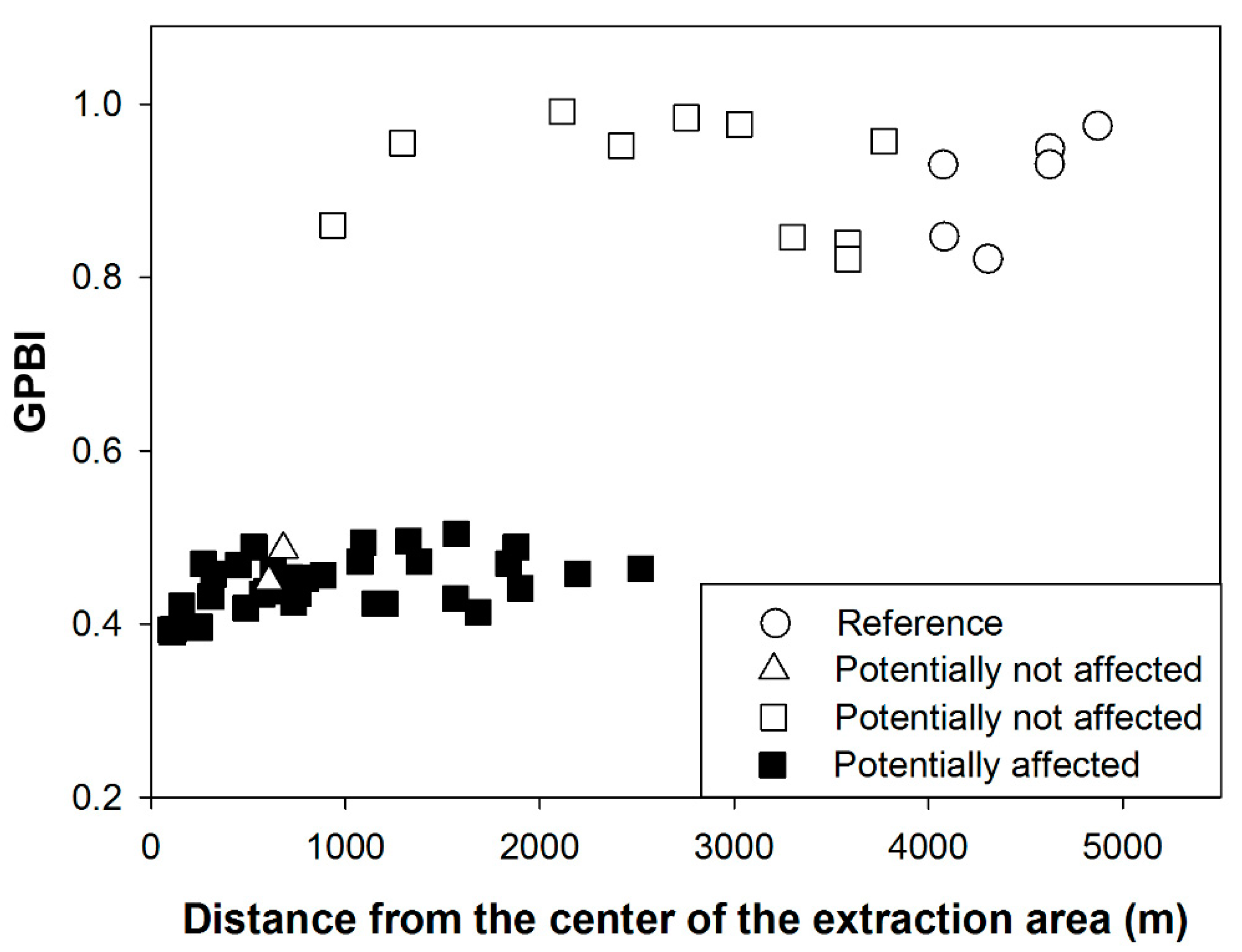
3.1.1. Case Study 1: Maerl Extraction (France, Bay of Biscay)

The relationship between the distance from the center of the maerl extraction area and GPBI is shown in Figure 2. The null hypothesis of no difference in GPBI between potentially affected stations on one hand and potentially not affected and reference stations on the other hand was rejected (p < 0.001, Kruskal–Wallis test; Table 2). Median GPBI was lower for potentially affected stations (0.45) than for potentially not affected (0.91) and reference stations (0.93). Interestingly the two potentially not affected stations represented by a triangle in Figure 1 were the closest to the extraction area and exhibited low GPBI values similar to those of potentially affected stations.

TDI also showed significant differences between groups (p = 0.016, Kruskal–Wallis test; Table 2) with median values of 1.09 and 0.80 for potentially not affected (including references) and potentially affected stations, respectively. Conversely, M-AMBI showed no difference between potentially affected stations and potentially not affected and reference (p = 0.847; Table 2, Supplementary Material S4).

3.1.2. Case Study 2: Dredge Disposal Pressure (Belgium, North Sea)

The relationships between the volume of disposed sediment and GPBI are shown in Figure 3A–C respectively for the three habitat types (Abra alba, Limecola balthica, and Nephtys cirrosa communities) and for each year separately. In each case, the stations submitted to the highest volume of sediment presented the lowest values of GPBI (Conover test, p < 0.05; Table 1).

In the Abra alba community (Figure 3A), the stations submitted to an intermediate level of sediment disposal had intermediate values of GPBI, significantly different from the reference stations in 2010 (0.61 ± 0.14 vs. 0.79 ± 0.05), 2011 (0.71 ± 0.14 vs. 0.96 ± 0.06), and 2012 (0.40 ± 0.15 vs. 0.81 ± 0.10), but not in 2008 (0.89 ± 0.11 vs. 0.91 ± 0.09; Conover tests, p = 0.72; Table 2).

In the Limecola balthica community, in 2008 there was no difference in GPBI between the reference and the intermediate level of pressure (Figure 3B, Table 2), but the highly impacted stations showed lower values than the reference (0.79 ± 0.07 vs. 0.90 ± 0.05). In 2010, there was a significant difference in GPBI values between the levels of pressure (Figure 3B₂, Table 2): the intermediately impacted stations showed the lowest values of GPBI (0.87 ± 0.20) while there was no significant difference between reference and highly impacted stations (0.90 ± 0.05 vs. 0.96 ± 0.09). For the 2011 subset, there was no difference in GPBI between pressure levels. In the subsequent year, the GPBI values of the impacted stations (0.39 ± 0.30 and 0.39 ± 0.32 for the intermediately and highly impacted stations, respectively) were significantly lower than that of the reference stations (0.95 ± 0.03) (Figure 3B₃ and B₄, Table 2).

In the Nephtys cirrosa community there was no difference in GPBI between the three levels of pressure for the 2008, 2010, and 2011 subsets (Figure 3C₁, C_2, and C₃; p > 0.05 in all cases, Kruskal–Wallis test; Table 2). In 2012, a significant difference between groups with a significantly lower GPBI for intermediate disturbance level (0.48 ± 0.10) was detected (Table 2). GPBI values were 0.80 ± 0.10 and 0.82 ± 0.21 for the reference and the highly impacted stations, respectively.

The detailed values and figures for M-AMBI and TDI are presented in Supplementary Material S5 and S6. In summary, the Kruskal–Wallis tests revealed that the null hypothesis of no difference between levels of pressure was rejected for only four subsets: Abra 2008, 2011, and 2012 and Nephtys 2011 with M-AMBI and Abra 2008, 2010, and 2011 and Nephtys 2010 with TDI.

For the Abra community, in 2008 the three levels of pressures presented significantly decreasing median values of M-AMBI with increasing fishing pressure (p < 0.01 in all cases, Conover test). In 2011, the high disturbance level was significantly different from the reference (p = 0.024, Conover test), and in 2012, it was significantly different from the intermediate level (p = 0.001, Conover test). In these two cases, the high disturbance level presented the lowest value of M-AMBI (0.40 ± 0.10 and 0.50 ± 0.07, respectively). For the Nephtys community in 2011, the high disturbance level was significantly different from the reference, but the M-AMBI median values of the index increased with increasing fishing pressure (Table 2, Supplementary Material S5).

In the Abra community, in 2008 and 2010, the three levels of pressures presented decreasing median values of TDI with increasing fishing pressure (Table 2, Supplementary Material S6). In 2008, the TDI values of the high disturbance level were significantly lower (0.34 ± 0.07) than those of intermediate level (0.67 ± 0.22) and reference (0.89 ± 0.23). The same pattern was observed in 2010. On the contrary, in the Nephtys community, in 2010, the reference stations showed TDI values significantly lower (0.76 ± 0.26) than the fished stations (1.32 ± 0.20 and 1.12 ± 0.29 for stations with intermediate and high levels of disturbance, respectively).

3.1.3. Case Study 3: Trawling Pressure (Germany, North Sea)

For each sampling occasion, clear differences in GPBI between the reference stations and the trawled stations could be detected (Figure 4, Table 2), except in April 2004 where three levels had to be considered. Here, three stations showed low GPBI values related to fishing pressure = 0 but were located in one of the fished zones. Therefore, the three levels considered were the following: (1) null trawling intensity in the unfished area, (2) null trawling intensity in the fished area (i.e., three lowest values in Figure 4), and (3) trawling intensity = 0.17 in the fished area. The difference between the last two levels was not significant (p = 0.931, Conover test). Reference station GPBI values were always higher than 0.83 (with one exception in April 2004 with GPBI = 0.71), while those of stations located in the trawled area were always lower than 0.83 (with one exception in July 2004 and one in September 2014 for which GPBI values were 0.97 and 0.93, respectively).

The null hypothesis of no difference in M-AMBI values between levels of trawling intensity was rejected in March 2003, November 2003, and April 2004 (Table 2, Supplementary Material S7), but in all these subdatasets, the M-AMBI showed higher values for the impacted stations than for the reference stations, which would indicate better EcoQ for stations located in the trawled area. The same absence of correlation is observed with the TDI values except in September 2004 (Supplementary Material S8): TDI values at reference stations 1.17 ± 0.12 while they were 0.97 ± 0.11 in the fished area (different levels of pressure are pooled) at this date.

3.1.4. Case Study 4: Hypoxia (Sweden, Gullmarfjord)

Temporal changes in GPBI values in the Gullmarfjord are shown in Figure 5. There were three major drops in GPBI values in 1980, 1989, and 1997–1998. A minimal GPBI value of 0.25 was recorded during the 1997–1998 event which took place after an exceptionally long period of anoxia. GPBI values recorded at the end of the recovery phases following each of the three hypoxia events were much lower than those recorded at the reference sampling dates. By defining two levels of pressure (i.e., impacted vs. not impacted) based on the threshold of 2 mL L⁻¹ of O₂ concentration during the year preceding each sampling date, there was a significant difference in both GPBI and M-AMBI between the two levels (p < 0.001 in both cases; Table 2). TDI values also show a significant difference between impacted stations (0.30 ± 0.41) and the unimpacted ones (0.87 ± 0.07). It has to be noted that only 11 stations have more than 50% of abundance with corresponding functional traits and are used for this analysis (i.e., 54 occasions are used to compute GPBI and M-AMBI (Table 2, Supplementary Material S9)).

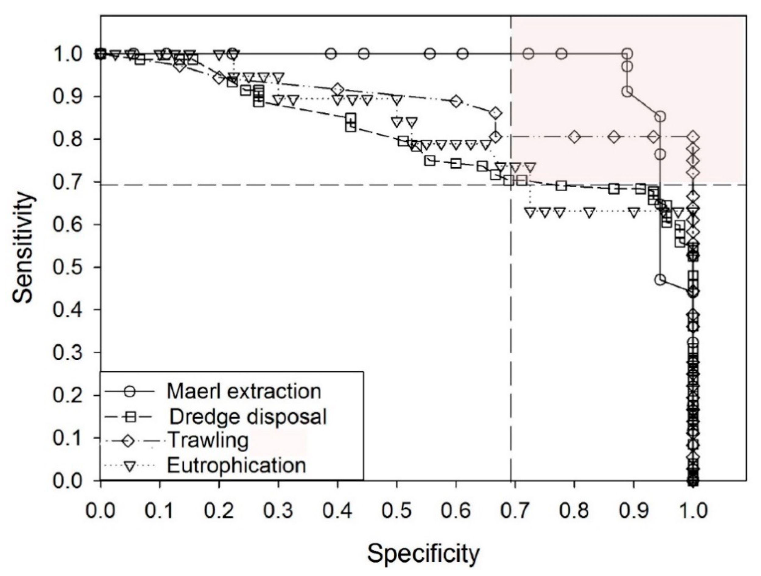
3.2. Performance of GPBI and Assessment of the Boundary between Good and Moderate EcoQ

The ROC curves obtained with the different datasets are presented in Figure 6. The area under the curve (AUC) was 0.91 for the maerl extraction dataset, 0.82 for the trawling dataset, 0.78 for the dredging dataset, and 0.80 for the hypoxia dataset. Cut-off values corresponding to specificity and sensitivity ≥ 0.7 correspond to the dots located in the grey area. They were obtained by computing the specificity and sensitivity values with values of cut-off contained in the following ranges: 0.47–0.84 for maerl extraction dataset, 0.78–0.91 for the trawling dataset, 0.80 for the dredging (only one square is in the gray area), and 0.38–0.42 for the hypoxia dataset.

4. Discussion

4.1. Performance of the Indices and Ecological Consideration

The maerl extraction case study demonstrates that the GPBI adequately detects physical disturbances. Still, two of the seven potentially not affected stations have low GPBI values. These low GPBI values can be interpreted as bad EcoQ, in contradiction with the Telemac-2D hydro-sedimentary mode. These stations are within 3 km of the maerl extraction center and surrounded by stations located within the same depth range and classified as potentially affected (Figure 1). The fact that the model did not take wind—which can cause dispersion of suspended particles—into account could explain this discrepancy. In contrast, M-AMBI assessed all stations as being at high or good EcoQ, which confirms that it is not the most suitable biotic index for physical disturbance [45,46,47]. TDI seems efficient in detecting impacted stations, even if 35 stations could not be taken into account as they did not reach the thresholds set for inclusion in the evaluation (50% of abundance with traits of sensitivity to trawling).

Maerl extraction induces two kinds of physical pressure: (1) a direct and strong modification of the habitat resulting from the removal of the substratum at the extraction point and (2) an indirect pressure of fine sediment resedimentation at a larger spatial scale due to the dispersion of resuspended fine sediment during extraction. The sediment plume leads to granulometric changes and an increase in the silt–clay fraction. This in turn can induce reduced oxygen penetration and reduced habitat complexity through microhabitat clogging. This not only results in a decrease in species richness and abundance but also leads to changes in species composition such as the substitution of K-selected species by opportunistic ones (r-selected species), the substitution of hard-bottom species with soft-bottom ones, or the substitution of indigenous biota by alien species [48]. The substitution of hard-bottom species by soft-bottom species can alleviate reduction in species richness (replacement >> richness differences): alpha-diversity indices do not reflect the impact on maerl communities outside the extraction point. Likewise, M-AMBI is not detecting extraction impacts, as richness and Shannon values are largely not affected and the sensitivity/tolerance of species is not equivalent for organic enrichment and sediment disposal. The evaluation of sensitivity for TDI is more appropriate in this situation. The advantage of the GPBI in this case is its ability to focus on the loss of hard-substrate species and to ignore gains in soft-substrate species.

GPBI also outperformed M-AMBI in the dredge disposal case study. GPBI led to the detection of impacted stations for 8 out of 12 subsets, whereas M-AMBI and TDI detected only four and seven cases, respectively. None of the three tested indices were able to detect dredge disposal effects in four subsets (one in the Limecola community and three in the Nephtys community). Our results suggest a gradual sensitivity to dredging for different communities with (i) the Abra community as the most sensitive, (ii) the Limecola community as intermediately sensitive, and (iii) the Nephtys community as the least sensitive community. As suggested by Powilleit et al. [49], this could be due to the rapid recovery of some species associated with the Limecola and the Nephtys communities. These authors distinguished three types of responses to disposal: (1) organisms, mostly infauna, able to survive burial (L. balthica and N. hombergii); (2) species that are maintained by escaping, moving up to the sediment surface, or immigrating from unaffected nearby areas (e.g., Diastylis rathkei); and (3) sensitive taxa (e.g., Abra alba, Lagis koreni) characterized by low mobility and fragile protecting parts. Differences in recovery rates between communities were also highlighted by Bolam and Rees [50] and are reflected in our study by higher species richness at impacted stations than at reference stations in the Limecola and Nephtys communities. Early successional stages are characterized by previously present species together with several opportunistic species absent from the reference stations. However, for the Nephtys community, it is difficult to disentangle affected and nonaffected stations on the basis of species abundances (see Supplementary Material S10).

Bolam and Rees [50] also state that low-diversity, stressed systems may recover more rapidly from severe disturbances because there is always a local supply of initial colonizers. This is consistent with the higher species richness in the undisturbed Abra community (29.8 ± 9.0) compared to the Limecola (2.5 ± 1.1) and Nephtys (8.0 ± 4.1) communities. The higher species richness of the A. alba community could also explain the performance of GPBI, as there is a greater potential for species loss than in the two other communities.

GPBI also outperformed M-AMBI and TDI in the trawling case study. Figure 6 shows higher trawling intensity in July and September 2004 (in accordance with Dannheim et al. [33]) and that the stability of GPBI is in accordance with Jac et al. [51]. Indeed, these authors showed that “abrupt” changes in the value of biotic indices may occur only when certain abrasion intensity thresholds are crossed. In the case of deep circalittoral habitat (A5.25), they estimated the threshold of abrasion to reach the “adverse effect” state at 0.11 SAR year⁻¹ (swept area ratio per year). Here, we considered a trawling intensity of 0.02 times trawled per month as the reference (i.e., lowest intensity available for this date). GPBI shows significant losses at the station trawled with an intensity of 0.06. The threshold value here is between 0.02 and 0.06 times trawled per month, and within the same order of magnitude as that proposed by Jac et al. [51], although we recognize that there are caveats when comparing monthly and yearly fishing pressure because of seasonal variability. As in the research of Jac et al. [18], TDI values are barely higher in the low-fishing-effort area compared to the reference zone.

In the long run, trawling effects become manifest as shifts in community composition and structure: from long-lived to short-lived, from large-sized to small-sized, and from slow-growing to fast-growing species (e.g., [52,53,54]).

McLaverty et al. [55] drew attention to the interest of using large (>4 mm) instead of small (1–4 mm) macrofauna to detect bottom trawling. Indeed, they found that stronger relationships exist between trawling intensity and large rather than small macrofauna response, and they argued that small macrofauna are typically characterized by high density, diversity, and population growth rates, and their relative resilience to trawling may mask the response of the more sensitive macrofauna [55]. This is probably also the case in the work of Dannheim [31], who failed to highlight the consequences of trawling on infauna communities. GPBI is free of these hindrances because (1) it focuses only on within-species loss of individuals between the reference and the tested station, which considerably reduces the noise induced by abundant species present in both impacted and reference stations or, more specifically, by factors such as “opportunistic species” or recruitment and (2) in doing so it considers each species individually and not global parameters such as total abundance or total species richness.

In GPBI, it is assumed that species lose individuals (and may disappear) between the reference and the tested station because they are sensitive to a disturbance, but without any a priori statements about this sensitivity. In fact, some of these species could be collateral victims of changes in bioturbation disturbance, facilitation disappearance, competition for food resources, or predation [56]. Consequently, by taking all species in the community into account (i.e., sampled species), GPBI captures a part of the consequences of the (negative) interactions between species which are not detected by other indices. This may be one of the reasons why it is efficient in detecting physical disturbance.

It may sound like it is easier and more reliable to focus on large macrofauna, but this depends on the sampling gear used. Studies conducted with grabs, box corers, or dredges focus mainly on quantitative data of infauna (often of small size) with a relatively restricted spatial coverage [57], while benthic data from scientific bottom trawl surveys focus mainly on semiquantitative data of mega-epifauna and integrate assemblage compositions over large areas. The present study shows that GPBI is efficient in the first case. In the second case, indices based on biological traits specific to the consideration of pressure [18] or global biomass as suggested by Hiddink et al. [58] may be more suitable, but GPBI could also be tested on such cases. As these different approaches do not focus on the same ecological compartment, they are complementary and not competing.

GPBI also proved efficient in detecting the three major changes in community composition resulting from prolonged hypoxia events ([O₂] < 2 mL L⁻¹) in 1980, 1989, and 1997–1998 in the Gullmarfjord [34]. As expected, M-AMBI was also efficient in this context. Severe organic enrichment triggered by natural events can lead to changes in benthos that are analogous to those seen in organically polluted systems (e.g., [3,59,60]) for which the M-AMBI was primarily developed. TDI did not perform well, but only a few observations could be taken into account as a consequence of the poor match between the dataset and the functional trait table [16]. Further, this can also be related to the masking effect of resilient and high-density species ([55] see below). Here, the decrease in species richness is so important [35] that all indices that take it or the loss of species into account (GPBI, M-AMBI) can detect the hypoxia events compared to those that do not (TDI).

4.2. Boundary between Good and Moderate EcoQ

In all cases, the ROC curves were right-skewed in relation to the x = y axis, illustrating the relationship between the indicator (abiotic factor) and the response (GPBI). When the area under the curve (AUC) is 1, then for a given cut-off value the sensitivity and the specificity are equal to 1. In this case, all stations classified as impacted by the abiotic factors are detected as impacted by GPBI, and none of the unimpacted stations are detected as impacted. The abiotic factors corresponding to the unimpacted stations are the results of the Telemac-2D model for the maerl extraction dataset, a null dredging intensity (based on real dredge volumes) for the dredge disposal dataset, and a null trawling intensity (based on VMS data) for the trawling dataset. For the eutrophication dataset, unimpacted stations are the ones with O₂ concentrations greater than 2 mL L^–1 the year before sampling.

The maerl case study (AUC = 0.91) reflects a strong agreement between the assessment of EcoQ with the Telemac-2D model and GPBI. The a priori classification of stations as potentially impacted or potentially not impacted is near-optimal since the model takes into account several parameters (hydrodynamics in terms of both tide currents and swell) adjusted to the local context although minor inconsistencies could arise (e.g., wind, see above). This dataset presents the inconvenience of its advantages: impacted stations are so clearly impacted that it lacks stations with intermediate values of GPBI, which results in a large range (0.47–0.84) of acceptable cut-off (sensitivity and specificity higher than 0.7). A more gradual response of the communities to maerl extraction could have helped us determine a clearer range of G/M EcoQ. However, it seems that maerl habitat complexity and fragility lead to rather abrupt shifts in the communities as opposed to gradual community change; such shifts rarely lead to any intermediate ecological status [61] but rather show binary response to physical pressure, even across continuous pressure gradients [62,63].

In the dredge disposal and the trawling case studies, the response of fauna was more gradual. The range of acceptable cut-off (those for which sensitivity and specificity are higher than 0.7) is thus smaller, with only one value (0.80) for the dredging dataset and a range of 0.78–0.91 for the trawling dataset.

In the Gullmarfjord, the effect of hypoxia (O₂ ≤ 2 mL L⁻¹) on macrofauna communities is well documented [39,64]. The results of our study (AUC = 0.80) agree well with results from other studies and thus provide evidence that GPBI is a good indicator for hypoxia: the Gullmarfjord dataset contains stations at different degrees of the succession, and GPBI is a proxy of changes in community structure. GPBI performed well, even though the “proxy” of pressure is still quite approximate as the average oxygen contents in the sediment per year are not calculated with continuous data but with punctuated data measured between 5 and 38 times a year (13 ± 5 data per year). Furthermore, the “shift” in community composition between the reference stations (before 1980) and the oxygenated period after 1980 results in values of GPBI always lower than 0.80. The range of cut-off for which sensitivity and specificity are higher than 0.7 is thus low: 0.38–0.42.

There is no clear consensus on one “best” cut-off amongst the four datasets. However, there are two main sources of uncertainty in the classification of stations as impacted or not impacted. The first is due to the binary logic of the method (for values close to the limit), and the second is that the shape of the ROC curve is also highly dependent on the choice of the abiotic good/moderate threshold itself [65]. According to our results, it is possible to conclude that a GPBI value lower than 0.38 indicates a bad EcoQ and a GPBI value higher than 0.80 indicates a good EcoQ. GPBI values between 0.38 and 0.80 are in fact representative of an intermediate EcoQ, and their classification depends more on the inherent resistance/resilience characteristics of the targeted habitat and thereby on the threshold which has to be chosen by considering the gain and loss in the performance of specificity and sensitivity within the ROC analysis. For example, choosing a threshold corresponding to a high sensitivity will cause a loss of some specificity. The cut-off of GPBI = 0.8 would be acceptable for all except the hypoxia case study. The limit of O₂ concentration should be set at 3.5 mL L⁻¹ to obtain a sensitivity and a specificity higher than 0.7. This cut-off at GPBI = 0.8 would classify only the reference stations as unimpacted. This corresponds to the nature of the dataset, which is a temporal series with a long-term trend of decreasing oxygen concentration superimposed on seasonal oxygen variations [66]. This highlights the importance of setting sound reference conditions and the moderate scientific robustness of “historical” references [67], since these gradual temporal changes may not be the targeted monitoring objectives [68].

We could thus propose the following boundaries: 0–0.4 would correspond to bad EcoQ, 0.4–0.7 would correspond to moderate EcoQ, 0.7–0.8 would correspond to good EcoQ, and 0.8–1.00 would correspond to very good EcoQ. The choice of a cut-off of 0.7 instead of 0.8 is the price of some specificity (and gain of some sensitivity). This kind of adjustment should be made by stakeholders based on the cost and gain of the consequences of this different classification.

Although the application of the signal detection theory approach (which requires pressure data) seems to be adequate, robust, and scientifically sound, as already reported by Chuševė et al. [69], it is crucial to further test GPBI and adjust boundaries within a larger variety of habitats and with varying pressures.

4.3. Recommendations for Future Sampling Designs

The present study clearly shows that the GPBI constitutes a promising tool for the quantitative assessments of the adverse effects of anthropogenic pressures on benthic habitats. The sound use of GPBI nevertheless requires that sampling designs follow some simple standard guidelines relating to the location, nature, and number of reference stations and to a sufficient sampling effort. In reality, these standard guidelines are not specific to GPBI. They are simply associated with the computation of its metric, whereas for most other biotic indices, constraints are often associated with the computation of EQR and/or EcoQ. The main recommendations can be summarized as follows:

• Since the computation of GPBI is based on the difference between benthic macrofauna composition and structure at a set of reference and tested stations, it is essential that these are located in the same habitat with similar natural environmental conditions and possibly within a limited geographical range. This condition is indeed necessary for the establishment of a sound relationship between the level of disturbance experienced by the tested station and its faunal composition. Such a habitat-based approach is also required for other biotic indices but is often associated with the stage of conversion of the metric in an EcoQ and not with the computation of the index itself. This issue is particularly important if monitoring areas are characterized by strong “natural” heterogeneity. Future monitoring surveys based on the use of GPBI should adopt a habitat-based sampling design.
• GPBI can be computed using a single reference or a set of reference stations. When using a single reference station, the GPBI of the reference will be 1. When using a set of reference stations, the GPBI of each reference will be 1 minus the difference of its value from the average of the values of GPBI of all reference stations. Results from the present study show that this value is usually slightly smaller than 1 (e.g., between 0.8 and 1 for the maerl case study). This reflects the “natural” variability in benthic macrofauna composition within the habitat of the tested station. Further, monitoring several reference stations allows for the detection of unexpected (local) habitat degradation occurring despite shifts of some of the reference stations. This still enables the assessment of a pressure effect using GPBI based on the remaining monitored references. Moreover, a predisturbance state would serve as a potential temporal reference which could then be compared with the states of the other reference stations. Again, this recommendation is not specific to GPBI, since (1) degradation of a single reference station would affect many biotic indices and (2) current biotic indices based on the assessment of the deviation from a reference state clearly (and explicitly) require a higher number of reference stations [70]. Our recommendation is thus to include several potential reference stations per habitat during future monitoring designs, whenever possible.
• Finding adequate reference stations clearly constitutes a major difficulty when using biotic indices due to the widespread and long-term alteration by pressures of marine coastal habitats, i.e., the problem of shifting baselines [11]. Sometimes, there is no other choice than choosing a “historical reference”, such as in the present Gullmarfjord case study. This is not the best situation because it is well known that coastal benthic ecosystems are shaped by seasonal and long-term dynamics [68,71,72,73]. Our general recommendation is therefore to monitor both potential reference and tested stations over longer time periods to disentangle natural from anthropogenic drivers for index quantification. The comparison of GPBI values between reference stations and the tested station would then allow for the assessment of the effects of local disturbances, whereas temporal changes in the GPBI values of reference stations would allow for the characterization of the effects of natural disturbances and/or long-term dynamics.

5. Conclusions

The present study is in accordance with the statement of Occam’s razor that “we are to admit no more causes of natural things, than such as are both true and sufficient to explain their appearances” (Newton, 1687). Indeed, the simple underlying assumption—that we can admit that macrofauna is impacted as soon as individuals of sensitive species begin to be lost—has proved to indicate correctly whether the stations have been impacted in four different case studies. Although GPBI needs to be tested further in order to check and adjust the boundaries between moderate and good EcoQ in different conditions, in a variety of different situations, and even with different ecological compartments, this index has shown to be a good candidate to be used in the frame of the European directives.

References

1. Van Hoey, G.; Borja, A.; Birchenough, S.; Buhl-Mortensen, L.; Degraer, S.; Fleischer, D.; Kerckhof, F.; Magni, P.; Muxika, I.; Reiss, H.; et al. The use of benthic indicators in Europe: From the Water Framework Directive to the Marine Strategy Framework Directive. Mar. Pollut. Bull. 2010, 60, 2187–2196. [Google Scholar] [CrossRef] [Green Version]
2. Diaz, R.J.; Solan, M.; Valente, R.M. A review of approaches for classifying benthic habitats and evaluating habitat quality. J. Environ. Manag. 2004, 73, 165–181. [Google Scholar] [CrossRef]
3. Pearson, T.H.; Rosenberg, R. Macrobenthic succession in relation to organic enrichment and pollution of the marine environment. Oceanogr. Mar. Biol. Annu. Rev. 1978, 16, 229–311. [Google Scholar]
4. Borja, Á.; Marín, S.L.; Muxika, I.; Pino, L.; Rodríguez, J.G. Is there a possibility of ranking benthic quality assessment indices to select the most responsive to different human pressures? Mar. Pollut. Bull. 2015, 97, 85–94. [Google Scholar] [CrossRef]
5. Grall, J.; Glémarec, M. Using Biotic Indices to Estimate Macrobenthic Community Perturbations in the Bay of Brest. Estuar. Coast. Shelf Sci. 1997, 44 (Suppl. A), 43–53. [Google Scholar] [CrossRef]
6. Borja, A.; Franco, J.; Pérez, V. A Marine Biotic Index to Establish the Ecological Quality of Soft-Bottom Benthos Within European Estuarine and Coastal Environments. Mar. Pollut. Bull. 2000, 40, 1100–1114. [Google Scholar] [CrossRef]
7. Borja, A.; Muxika, I.; Franco, J. The application of a Marine Biotic Index to different impact sources affecting soft-bottom benthic communities along European coasts. Mar. Pollut. Bull. 2003, 46, 835–845. [Google Scholar] [CrossRef]
8. Muxika, I.; Borja, A.; Bald, J. Using historical data, expert judgement and multivariate analysis in assessing reference conditions and benthic ecological status, according to the European Water Framework Directive. Mar. Pollut. Bull. 2007, 55, 16–29. [Google Scholar] [CrossRef]
9. Dauvin, J.C.; Ruellet, T. Polychaete/amphipod ratio revisited. Mar. Pollut. Bull. 2007, 55, 215–224. [Google Scholar] [CrossRef] [PubMed]
10. Dauvin, J.C.; Ruellet, T. The Estuarine Quality Paradox: Is it possible to define an Ecological Quality Status for specific modified and naturally stressed estuarine ecosystems? Mar. Pollut. Bull. 2009, 59, 38–47. [Google Scholar] [CrossRef]
11. Halpern, B.S.; Walbridge, S.; Selkoe, K.A.; Kappel, C.V.; Micheli, F.; D’Agrosa, C.; Bruno, J.F.; Casey, K.S.; Ebert, C.; Fox, H.E.; et al. A Global Map of Human Impact on Marine Ecosystems. Science 2008, 319, 948–952. [Google Scholar] [CrossRef] [PubMed] [Green Version]
12. Hiddink, J.G.; Jennings, S.; Kaiser, M.J. Assessing and predicting the relative ecological impacts of disturbance on habitats with different sensitivities. J. Appl. Ecol. 2007, 44, 405–413. [Google Scholar] [CrossRef]
13. Labrune, C.; Grémare, A.; Amouroux, J.-M.; Sardá, R.; Gil, J.; Taboada, S. Diversity of polychaete fauna in the Gulf of Lions (NW Mediterranean). Vie Et Milieu 2006, 56, 315–326. [Google Scholar]
14. Labrune, C.; Grémare, A.; Amouroux, J.-M.; Sardá, R.; Gil, J.; Taboada, S. Assessment of soft-bottom polychaete assemblages in the Gulf of Lions (NW Mediterranean) based on a mesoscale survey. Estuar. Coast. Shelf Sci. 2007, 71, 133–147. [Google Scholar] [CrossRef]
15. De Juan, S.; Demestre, M. A Trawl Disturbance Indicator to quantify large scale fushing impact on benthic ecosystems. Ecol. Indic. 2012, 18, 183–190. [Google Scholar] [CrossRef]
16. Foveau, A.; Vaz, S.; Desroy, N.; Kostylev, V.E. Process-driven and biological characterisation and mapping of seabed habitats sensitive to trawling. PLoS ONE 2017, 12, e0184486. [Google Scholar] [CrossRef] [Green Version]
17. Certain, G.; Jørgensen, L.L.; Christel, I.; Planque, B.; Bretagnolle, V. Mapping the vulnerability of animal community to pressure in marine systems: Disentangling pressure types and integrating their impact from the individual to the community level. ICES J. Mar. Sci. 2015, 72, 1470–1482. [Google Scholar] [CrossRef] [Green Version]
18. Jac, C.; Desroy, N.; Certain, G.; Foveau, A.; Labrune, C.; Vaz, S. Detecting adverse effect on seabed integrity. Part 1: Generic sensitivity indices to measure the effect of trawling on benthic mega-epifauna. Ecol. Indic. 2020, 117, 106631. [Google Scholar] [CrossRef]
19. Flåten, G.R.; Botnen, H.; Grung, B.; Kvalheim, O.M. Quantifying disturbances in benthic communities--comparison of the community disturbance index (CDI) to other multivariate methods. Ecol. Indic. 2007, 7, 254–276. [Google Scholar] [CrossRef]
20. Johnson, R.L.; Perez, K.T.; Rocha, K.J.; Davey, E.W.; Cardin, J.A. Detecting benthic community differences: Influence of statistical index and season. Ecol. Indic. 2008, 8, 582–587. [Google Scholar] [CrossRef]
21. de los Ríos, A.; Pérez, L.; Ortiz-Zarragoitia, M.; Serrano, T.; Barbero, M.C.; Echavarri-Erasun, B.; Juanes, J.A.; Orbea, A.; Cajaraville, M.P. Assessing the effects of treated and untreated urban discharges to estuarine and coastal waters applying selected biomarkers on caged mussels. Mar. Pollut. Bull. 2013, 77, 251–265. [Google Scholar] [CrossRef]
22. Ruggiero, A.; Lawton, J.H.; Blackburn, T.M. The geographic ranges of mammalian species in South America: Spatial patterns in environmental resistance and anisotropy. J. Biogeogr. 1998, 25, 1093–1103. [Google Scholar] [CrossRef]
23. Koleff, P.; Gaston, K.J.; Lennon, J.J. Measuring beta diversity for presence-absence data. J. Anim. Ecol. 2003, 72, 367–382. [Google Scholar] [CrossRef] [Green Version]
24. Legendre, P. Interpreting the replacement and richness difference components of beta diversity. Glob. Ecol. Biogeogr. 2014, 23, 1324–1334. [Google Scholar] [CrossRef]
25. Murtaugh, P.A. The Statistical Evaluation of Ecological Indicators. Ecol. Appl. 1996, 6, 132–139. [Google Scholar] [CrossRef] [Green Version]
26. Grall, J.; Hall-Spencer, J. Problems facing maerl conservation in Brittany. Aquat. Conserv. Mar. Freshw. Ecosyst. 2003, 13, S55–S64. [Google Scholar] [CrossRef]
27. De Grave, S.; Whitaker, A. A census of maerl beds in Irish waters. Aquat. Conserv. Mar. Freshw. Ecosyst. 1999, 9, 303–311. [Google Scholar] [CrossRef]
28. SOGREAH. Modélisation du panache turbide de l’extraction in in vivo. Etude et cartographie du banc de maerl du nord de l’archipel des Glénans. In Rapport Ville de Fouesnant; Rapport Ville de Fouesnant: Fouesnant, France, 2004; pp. 3–38. [Google Scholar]
29. Lauwaert, B.; De Witte, B.; Devriese, L.; Fettweis, M.; Martens, C.; Steve, T.; Van Hoey, G.; Vanlede, J. Synthesis Report on the Effects of Dredged Material Dumping on the Marine Environment (Licensing Period 2012–2016). 2016. Available online: https://www.researchgate.net/publication/311653421_Synthesis_report_on_the_effects_of_dredged_material_dumping_on_the_marine_environment_licensing_period_2012-2016 (accessed on 12 June 2021).
30. Breine, N.; Backer, A.; Van Colen, C.; Moens, T.; Hostens, K.; Van Hoey, G. Structural and functional diversity of soft-bottom macrobenthic communities in the Southern North Sea. Estuar. Coast. Shelf Sci. 2018, 214. [Google Scholar] [CrossRef]
31. Dannheim, J. Macrozoobenthic Response to Fishery—Trophic Interactions in Highly Dynamic Coastal Ecosystems. Ph.D. Dissertation, University of Bremen, Bremen, Germany, 2007. Available online: http://nbn-resolving.de/urn:nbn:de:gbv:46-diss000108658 (accessed on 31 July 2020).
32. Rijnsdorp, A.D.; Buys, A.M.; Storbeck, F.; Visser, E.G. Micro-scale distribution of beam trawl effort in the southern North Sea between 1993 and 1996 in relation to the trawling frequency of the sea bed and the impact on benthic organisms. ICES J. Mar. Sci. 1998, 55, 403–419. [Google Scholar] [CrossRef]
33. Dannheim, J.; Brey, T.; Schröder, A.; Mintenbeck, K.; Knust, R.; Arntz, W.E. Trophic look at soft-bottom communities—Short-term effects of trawling cessation on benthos. J. Sea Res. 2014, 85, 18–28. [Google Scholar] [CrossRef] [Green Version]
34. Josefson, A.B.; Blomqvist, M.; Hansen, J.L.S.; Rosenberg, R.; Rygg, B. Assessment of marine benthic quality change in gradients of disturbance: Comparison of different Scandinavian multi-metric indices. Mar. Pollut. Bull. 2009, 58, 1263–1277. [Google Scholar] [CrossRef]
35. Josefson, A.B.; Widbom, B. Differential response of benthic macrofauna and meiofauna to hypoxia in the Gullmar Fjord basin. Mar. Biol. 1988, 100, 31–40. [Google Scholar] [CrossRef]
36. Nilsson, H.C.; Rosenberg, R. Succession in marine benthic habitats and fauna in response to oxygen deficiency: Analysed by sediment profile-imaging and by grab samples. Mar. Ecol. Prog. Ser. 2000, 197, 139–149. [Google Scholar] [CrossRef]
37. Rosenberg, R.; Agrenius, S.; Hellman, B.; Nilsson, H.C.; Norling, K. Recovery of marine benthic habitats and fauna in a Swedish fjord following improved oxygen conditions. Mar. Ecol. Prog. Ser. 2002, 234, 43–53. [Google Scholar] [CrossRef]
38. Polovodova Asteman, I.; Nordberg, K. Foraminiferal fauna from a deep basin in Gullmar Fjord: The influence of seasonal hypoxia and the North Atlantic Oscillation. J. Sea Res. 2013, 79, 40–49. [Google Scholar] [CrossRef]
39. Gogina, M.; Darr, A.; Zettler, M.L. Approach to assess consequences of hypoxia disturbance events for benthic ecosystem functioning. J. Mar. Syst. 2014, 129, 203–213. [Google Scholar] [CrossRef]
40. Bald, J.; Borja, A.; Muxika, I.; Franco, J.; Valencia, V. Assessing reference conditions and physico-chemical status according to the European Water Framework Directive: A case-study from the Basque Country (Northern Spain). Mar. Pollut. Bull. 2005, 50, 1508–1522. [Google Scholar] [CrossRef]
41. Foveau, A.; Jac, C.; Llpasset, M.; Guillerme, C.; Desroy, N.; Vaz, S. Updated Biological Traits’ Scoring and Protection Status to Calculate sensItivity to Trawling on Mega-Epibenthic Fauna. 2019. Available online: https://agris.fao.org/agris-search/search.do?recordID=QN2019001269067 (accessed on 12 June 2021).
42. Conover, W.J.; Iman, R.L. On Multiple-Comparisons Procedures; Tech. Rep. LA-7677-MS; Los Alamos Scientific Laboratory: New Mexico, NM, USA, 1979. [Google Scholar]
43. Hale, S.S.; Heltshe, J.F. Signals from the benthos: Development and evaluation of a benthic index for the nearshore Gulf of Maine. Ecol. Indic. 2008, 8, 338–350. [Google Scholar] [CrossRef]
44. Hosmer, D.; Lemeshow, S. Applied Logistic Regression, 2nd ed.; John Wiley Sons Inc.: New York, NY, USA, 2000; 375p. [Google Scholar] [CrossRef]
45. Fitch, J.E.; Cooper, K.M.; Crowe, T.P.; Hall-Spencer, J.M.; Phillips, G. Response of multi-metric indices to anthropogenic pressures in distinct marine habitats: The need for recalibration to allow wider applicability. Mar. Pollut. Bull. 2014, 87, 220–229. [Google Scholar] [CrossRef] [PubMed]
46. Labrune, C.; Amouroux, J.M.; Sardá, R.; Dutrieux, E.; Thorin, S.; Rosenberg, R.; Grémare, A. Characterization of the ecological quality of the coastal Gulf of Lions (NW Mediterranean). A comparative approach based on three biotic indices. Mar. Pollut. Bull. 2006, 52, 34–47. [Google Scholar] [CrossRef]
47. Teixeira, H.; Salas, F.; Neto, J.M.; Patrício, J.; Pinto, R.; Veríssimo, H.; García-Charton, J.A.; Marcos, C.; Pérez-Ruzafa, A.; Marques, J.C. Ecological indices tracking distinct impacts along disturbance-recovery gradients in a temperate NE Atlantic Estuary-Guidance on reference values. Estuar. Coast. Shelf Sci. 2008, 80, 130–140. [Google Scholar] [CrossRef]
48. Barbera, C.; Bordehore, C.; Borg, J.; Glémarec, M.; Grall, J.; Hall-Spencer, J.M.; de la Huz, C.; Lanfranco, E.; Lastra, M.; Moore, P.; et al. Conservation and management of northeast Atlantic and Mediterranean maerl beds. Aquat. Conserv Mar. Freshw. Ecosyst. 2003, 13, S65–S76. [Google Scholar] [CrossRef]
49. Powilleit, M.; Kleine, J.; Leuchs, H. Impacts of experimental dredged material disposal on a shallow, sublittoral macrofauna community in Mecklenburg Bay (western Baltic Sea). Mar. Pollut. Bull. 2006, 52, 386–396. [Google Scholar] [CrossRef]
50. Bolam, S.G.; Rees, H.L. Minimizing Impacts of Maintenance Dredged Material Disposal in the Coastal Environment: A Habitat Approach. Environ. Manag. 2003, 32, 171–188. [Google Scholar] [CrossRef] [PubMed]
51. Jac, C.; Desroy, N.; Certain, G.; Foveau, A.; Labrune, C.; Vaz, S. Detecting adverse effect on seabed integrity. Part 2: How much of seabed habitats are left in good environmental status by fisheries? Ecol. Indic. 2020, 117, 106617. [Google Scholar] [CrossRef]
52. Dayton, P.; Thrush, S.; Agardy, T.; Hofman, R. Environmental effects of marine fishing. Aquat. Conserv. -Mar. Freshw. Ecosyst. 1995, 5, 205–232. [Google Scholar] [CrossRef]
53. Hiddink, J.; Jennings, S.; Kaiser, M.; Queiros, A.; Duplisea, D.E.; Piet, G. Cumulative Impacts of Seabed Trawl Disturbance on Benthic Biomass, Production, and Species Richness in Different Habitats. Can. J. Fish. Aquat. Sci. 2006, 63, 721–736. [Google Scholar] [CrossRef]
54. Reise, K. Long-term changes in the macrobenthic invertebrate fauna of the Wadden Sea: Are Polychaetes about to take over? Neth. J. Sea Res. 1982, 16, 29–36. [Google Scholar] [CrossRef]
55. McLaverty, C.; Eigaard, O.R.; Gislason, H.; Bastardie, F.; Brooks, M.E.; Jonsson, P.; Lehmann, A.; Dinesen, G.E. Using large benthic macrofauna to refine and improve ecological indicators of bottom trawling disturbance. Ecol. Indic. 2020, 110, 105811. [Google Scholar] [CrossRef]
56. van de Wolfshaar, K.E.; van Denderen, P.D.; Schellekens, T.; van Kooten, T. Food web feedbacks drive the response of benthic macrofauna to bottom trawling. Fish Fish. 2020, 21, 962–972. [Google Scholar] [CrossRef]
57. van Loon, W.M.G.M.; Walvoort, D.J.J.; van Hoey, G.; Vina-Herbon, C.; Blandon, A.; Pesch, R.; Schmitt, P.; Scholle, J.; Heyer, K.; Lavaleye, M.; et al. A regional benthic fauna assessment method for the Southern North Sea using Margalef diversity and reference value modelling. Ecol. Indic. 2018, 89, 667–679. [Google Scholar] [CrossRef]
58. Hiddink, J.; Kaiser, M.; Sciberras, M.; McConnaughey, R.; Mazor, T.; Hilborn, R.; Collie, J.; Pitcher, C.; Parma, A.; Suuronen, P.; et al. Selection of indicators for assessing and managing the impacts of bottom trawling on seabed habitats. J. Appl. Ecol. 2020, 57. [Google Scholar] [CrossRef]
59. Birchenough, S.N.R.; Frid, C.L.J. Macrobenthic succession following the cessation of sewage sludge disposal. J. Sea Res. 2009, 62, 258–267. [Google Scholar] [CrossRef]
60. Diaz, R.J.; Rosenberg, R. Spreading Dead Zones and Consequences for Marine Ecosystems. Science 2008, 321, 926. [Google Scholar] [CrossRef] [PubMed]
61. Hall-Spencer, J.M. Conservation issues concerning the molluscan fauna of maerl beds. J. Conchol. Spec. Publ. 1998, 2, 271–286. [Google Scholar]
62. Hall-Spencer, J.; Moore, P. Scallop dredging has profound, long-term impacts on maerl habitats. J. Mater. Sci. 2000, 57, 1407–1415. [Google Scholar] [CrossRef] [Green Version]
63. Bernard, G.; Romero-Ramirez, A.; Tauran, A.; Pantalos, M.; Deflandre, B.; Grall, J.; Grémare, A. Declining maerl vitality and habitat complexity across a dredging gradient: Insights from in situ sediment profile imagery (SPI). Sci. Rep. 2019, 9, 16463. [Google Scholar] [CrossRef] [PubMed]
64. Alve, E.; Lepland, A.; Magnusson, J.; Backer-Owe, K. Monitoring strategies for re-establishment of ecological reference conditions: Possibilities and limitations. Mar. Pollut. Bull. 2009, 59, 297–310. [Google Scholar] [CrossRef] [PubMed]
65. Connors, B.M.; Cooper, A.B. Determining Decision Thresholds and Evaluating Indicators when Conservation Status is Measured as a Continuum. Conserv. Biol. 2014, 28, 1626–1635. [Google Scholar] [CrossRef]
66. Erlandsson, C.P.; Stigebrandt, A.; Arneborg, L. The sensitivity of minimum oxygen concentrations in a fjord to changes in biotic and abiotic external forcing. Limnol. Oceanogr. 2006, 51, 631–638. [Google Scholar] [CrossRef]
67. Borja, Á.; Dauer, D.M.; Grémare, A. The importance of setting targets and reference conditions in assessing marine ecosystem quality. Ecol. Indic. 2012, 12, 1–7. [Google Scholar] [CrossRef]
68. Kröncke, I.; Reiss, H. Influence of macrofauna long-term natural variability on benthic indices used in ecological quality assessment. Mar. Pollut. Bull. 2010, 60, 58–68. [Google Scholar] [CrossRef]
69. Chuševė, R.; Nygård, H.; Vaičiūtė, D.; Daunys, D.; Zaiko, A. Application of signal detection theory approach for setting thresholds in benthic quality assessments. Ecol. Indic. 2016, 60, 420–427. [Google Scholar] [CrossRef] [Green Version]
70. Lavesque, N.; Blanchet, H.; De Montaudouin, X. Development of a multimetric approach to assess perturbation of benthic macrofauna in Zostera noltii beds. J. Exp. Mar. Biol. Ecol. 2009, 368, 101–112. [Google Scholar] [CrossRef]
71. Dauvin, J.-C. The Muddy Fine Sand Abra alba-Melinna palmata Community of the Bay of Morlaix Twenty Years After the Amoco Cadiz Oil Spill. Mar. Pollut. Bull. 2000, 40, 528–536. [Google Scholar] [CrossRef]
72. Labrune, C.; Grémare, A.; Guizien, K.; Amouroux, J.M. Long-term comparison of soft bottom macrobenthos in the Bay of Banyuls-sur-Mer (Northwestern Mediterranean Sea): A reappraisal. J. Sea Res. 2007, 58, 125–143. [Google Scholar] [CrossRef]
73. Romero-Ramirez, A.; Bonifácio, P.; Labrune, C.; Sardá, R.; Amouroux, J.M.; Bellan, G.; Duchêne, J.C.; Hermand, R.; Karakassis, I.; Dounas, C.; et al. Long-term (1998–2010) large-scale comparison of the ecological quality status of gulf of lions (NW Mediterranean) benthic habitats. Mar. Pollut. Bull. 2016, 102, 102–113. [Google Scholar] [CrossRef] [PubMed] [Green Version]
Figure 1. Map showing the locations of the 4 case studies: (A) maerl extraction in the Glénan Archipelago, (B) dredging on the Belgium coast, (C) trawling in the German Bight (North Sea) (D), and the station submitted to hypoxia in the Gullmarfjord.
Jmse 09 00654 g001
Figure 2. Case Study 1—maerl extraction in Glénan Archipelago (France, northern Bay of Biscay). Relationships between pressure levels, as indicated by geographical distances from the center of the maerl extraction area, and GPBI.
Jmse 09 00654 g002
Figure 3. Case Study 2—dredge disposal (Belgium, North Sea). Relationship between the volumes dredged as intermediate and high versus GPBI for the Abra alba community in 2008 (A1), 2010 (A2), 2011 (A3), and 2012 (A4); the Limecola balthica community in 2008 (B1), 2010 (B2), 2011 (B3), and 2012 (B4); and the Nephtys cirrosa community in 2008 (C1), 2010 (C2), 2011 (C3), and 2012 (C4).
Jmse 09 00654 g003
Figure 4. Case Study 3—trawling pressure (Germany, North Sea). Relationship between the fishing pressure (SAR, times trawled month−1) and the GPBI for the stations located in two fishing areas and the unfished area in the German Bight (North Sea)(A) in March 2003, (B) in November 2003, (C) in April 2004, (D) in July 2004 and (E) in September 2004.
Jmse 09 00654 g004
Figure 5. Case Study 4—hypoxia (Sweden, Gullmarfjord). Temporal changes in GPBI. The sampling dates used as references are indicated by a white square. Shaded areas are indicative of hypoxia events ([O2] < 2 mL L−1).
Jmse 09 00654 g005
Figure 6. ROC curves for the four case studies. Sensitivity and specificity were computed with increasing cut-off of GPBI between 0 and 1 by 0.01. The “real” impact of stations was based on (1) distance to maerl extraction by Telemac-2D hydro-sedimentary model, (2) dredged sediment volume (zero vs. < zero), (3) fishing pressure zero in unfished area vs. > zero in fished areas, and (4) O2 concentration (average concentration less or greater than 2 mL L–1 the year before sampling). For further details, please see Section 2.
Jmse 09 00654 g006