ANN-Based Decision Making in Station Keeping for Geotechnical Drilling Vessel

Abstract

Offshore vessels (OVs) often require precise station-keeping and some vessels, for example, vessels involved in geotechnical drilling, generally use Spread Mooring (SM) or Dynamic Positioning (DP) systems. Most of these vessels are equipped with both systems to cover all ranges of water depths. However, determining which system to use for a particular operational scenario depends on many factors and requires significant balancing in terms of cost-benefit. Therefore, this research aims to develop a platform that will determine the cost factors for both the SM and DP station-keeping systems. Operational information and cost data are collected for several field operations, and Artificial Neural Networks (ANN) are trained using those data samples. After that, the trained ANN is used to predict the components of cost for any given environmental situation, fieldwork duration and water depth. Later, the total cost is investigated against water depth for both DP and SM systems to determine the most cost-effective option. The results are validated using two operational scenarios for a specific geotechnical vessel. This decision-making algorithm can be further developed by adding up more operational data for various vessels and can be applied in the development of sustainable decision-making business models for OVs operators.

1. Introduction

The ever-increasing demand for energy and food with the rise of the population has intensified numerous offshore activities more than ever. Various OVs play an integral part in these offshore operations by supporting installation, maintenance, supplies, accommodations and other similar activities. One such vessel is geotechnical survey vessels, which play a critical role in the discovery and development of offshore fields. The geotechnical vessel’s primary function is to collect a soil sample below the seabed, usually up to 300 m deep. The samples are collected from pre-specified locations, and the vessel is connected to the seabed during this operation through drill pipes and seabed frame. Any movement of the vessel from the desired position may jeopardize the operation and cause severe safety, health, environmental, and of course, financial damages. Therefore, station-keeping is crucial for a geotechnical drilling vessel, and usually, it is achieved either by DP or SM.

DP means a vessel’s ability to maintain its position and heading using a computer-based controlled programme by means of sensing environmental conditions, signal processing, and electronic commands to propellers, thrusters and rudders [1]. Generally, the DP system becomes less effective in shallow water because of the wider DP footprint; also, position reference systems are a limiting factor in shallow water DP operations [2]. Shallow water DP operation may also cause seabed mud and sand interference to propellers and thrusters, thus impacting underwater machinery integrity. Therefore, a geotechnical vessel with only a DP system is not ideal for operating in shallow water, whereas it is a preferred choice for Deepwater operation.

On the other hand, SM is positioning a vessel in a specific location by securing it to the seabed using multiple numbers of mooring lines and anchors. The bow is typically heading towards a dominant environment where the largest waves or wind is expected. The propulsion system can be utilized to control the vessel’s heading to reduce position offset and forces in the mooring lines [3]. The spread mooring system is suitable for shallow water but not a suitable option for deep waters. The system requires significant wire length in the seabed and at least 40% of wires in the drum after reaching a final position to minimize reaction forces on the winch and vessel structure. Besides, increased wire length may require an increased diameter of the wire to withstand the large forces. This will result in massive winches and ample deck space [4].

A geotechnical vessel operates across various water depth regions ranging from shallow to deep waters. While the choice of station-keeping for very shallow and very deep water is relatively straightforward, the decision on station-keeping choice in an intermediate water depth region varies significantly between geotechnical vessels. This is because a geotechnical vessel’s operational period in a particular location is temporary, usually several hours to days. Therefore, depending on several variables, including fuel cost, activity duration, environments, both the DP and SM, can be a cost-effective solution for particular water depth. As a result, most geotechnical vessel operators prefer to install both the DP and SM systems on their vessels.

Extensive research on DP modelling and operations from technical and scientific points of view have been performed by many researchers over the past two decades [5,6]. Similarly, simulation and prediction of motion control and station-keeping of both surface and underwater vessels has received significant attention during the same period. For example, motion analysis of coupled unmanned surface vehicles and underwater vehicles [7], modelling the motion behaviour of underwater vehicles while connected with umbilical [8], performance and stability simulation of hovering over-actuated autonomous underwater vehicle (HAUV) robust station-keeping (SK) control algorithm under model uncertainties and ocean current disturbance in the horizontal plane [9].

However, considering commercial perspective, no published guidelines exist on when to use DP or SM to ensure a sustainable and cost-effective operation taking into account all the operational variables during a project. At present, the operators usually go through a complex project assessment and calculation phase to decide on station-keeping. Taking advantage of past projects information, this study, however, aims to propose an efficient, ANN-based decision-making model for station-keeping of geotechnical vessels. ANN is widely used by researchers to solve numerous problems where conventional modelling methods fail [10], as it can accommodate multiple input variables to predict multiple output variables. In this study, the ANN model is developed by focusing on the total, overall operational cost only, which can be further developed by including other factors in the future. Various data, including Fuel Oil (FO) consumption, duration, and environmental conditions, are collected for an existing geotechnical vessel from past projects. ANN is then implemented to learn the relationship among the variables and later to predict the operational cost for a given weather condition and water depth at a particular project location. The trained ANN model is also validated against two recent project data to ensure the accuracy of the decision-making process.

2. Methodology

This research aims to establish a decision-making platform to determine whether the SM or DP system is more economical for a geotechnical vessel’s station-keeping at a particular location, keeping the associated operating variable and their limits in mind. Therefore, the first step of the workflow is to identify the key variables that will impact SM and DP’s operating cost, followed by vessel selection and data collection. The systematic approaches followed in this work are summarized in the following steps:

2.1. Identifying the Common Variables for Both the DP and SM System

The first and most significant and critical task for this project is identifying the variables based on which the cost analyses will be performed to develop the decision-making process. For geotechnical vessels, both the DP and the SM system have sets of variables that affect overall cost and efficiency. However, to develop that comparative decision-making platform between the two options, it is crucial to recognize the set of common variables that would impact the comparison process. Hence, one-on-one interview and focus group discussions with academics, colleagues in the industry, vessel crews (Captain, Chief Engineer) were performed. The findings were analyzed by the authors to identify all the major variables influencing the decision-making process.

Table 1. Identified variables for DP and SM systems.

	DP System	SM System
i. Environmental Factors
Significant wave	X	X
Current	X	X
Wind	X	X
Wave period	X	X
Drilling depth	X	X
Water depth	X	X
Mooring length	N/A	X
ii. Cost Factors
FO consumption	X	X
Compliance cost	X	X
Additional crew	X	N/A
Spares	X	X
iii. Time Factors
Time for positioning	X	X
Time for de-positioning	N/A	X
Weather standby	X	X
Emergency response	X	X

shows the identified variables for both systems under three main categories.

It is important to note that all these variables listed in Table 1 will impact the operating cost of the geotechnical drilling vessel. However, there are some variables for which both the DP and SM systems will incur similar costs. Hence, those variables will not significantly impact the decision-making process and will be disregarded during the data collection phase of this study.

For example, under the environmental factor, water depth has a variable impact on station-keeping in terms of cost and time for both the DP and SM systems. However, the influence of drilling depth on cost and efficiency will not significantly differ between both systems. So, drilling depth was not considered for data collections. Factors, for example, wave period, current, wind, were combined and expressed as an Environmental Regularity Number (ERN). ERN is a theoretical way of defining a vessel’s ability to maintain its position in different weather and sea conditions. It was developed in the 1970s by Det Norske Veritas (DNV), and more details can be found here: [11]. ERN calculations assume that the forces resulting from wind, waves and current are coincident, with the magnitudes of wind and waves being of equal probability and are intended to reflect a ‘worst-case situation’. A guidance note by DNV says this is normally when the weather is on the vessel’s beam, and the ERN is based on this situation “regardless of the vessel’s ability to select other headings in operation”. An ERN number of ‘zero’ means calm water condition.

Similarly, the costs for compliance and spares are similar for both the DP and SM systems, hence considering not impacting the decision-making process. Therefore, only the cost for Fuel Oil (FO) consumption and additional crew for DP operation is calculated and modelled. Under the time factors, weather standby and emergency response are not considered in this research as weather standby is somewhat unpredictable, and emergency response for SM is quite complicated. Therefore, only the time required for positioning and de-positioning are collected, analyzed, and converted to monetary contributions on the vessel’s total operating cost.

2.2. Vessel Selection for Data Collection

A geotechnical vessel with principal particulars shown in

Table 2. Principal particulars of the geotechnical vessel under consideration.

Particulars	Values
Length overall	76.0 m
Beam (mid)	20.0 m
Depth Moulded	6.1 m
Draft	4.7 m
Displacement	4746 tons
Speed	Max. 12 knots
Endurance	Max. 42 days
Operational Water Depth	10 m to 1000 m (seabed operations)

is selected for this study. This vessel is part of the fleet managed and operated by Fugro. It was built in 2007 as an Offshore Supply Vessel (OSV) and later converted to a geotechnical drilling vessel by performing all necessary modifications and installing machinery required for drilling. The vessel is currently operating in the Asia Pacific Region and fitted with both DP and SM systems. It has a DP2 system with station-keeping as the primary function. This DP system can also be used for manoeuvring by employing the C-Joy system and target tracking. The four-point SM system has a total anchor wire length of 2000 m, and the system can perform self-anchoring if there is no physical obstruction on the anchoring spread.

2.3. Data Collection and Understanding Associated Limitations

The vessels’ location-specific and operational data were collected with help from the Master and Chief Engineer of the vessel, colleagues from the computerized Planned Maintenance System (PMS) and Computerised Management System (CMS) working in Fugro headquarters in the Netherlands. A systematic approach is applied to collect the data, for example, water depth, environmental conditions, FO consumption and other cost factors, time consumed for various operations, for various site-specific projects which are already completed. All the data were collected from projects which are done within a two year span after a special survey. The time frame is crucial as data collected (especially the FO consumption) from projects spread over a much longer time might not be suitable for decision-making modelling. This is due to the fouling formed on the hull and the deterioration of anti-fouling paint over time.

During DP operation, two azimuth thrusters, two bow thrusters, two main engines, two shaft generators and two auxiliary engines were in operation. The second auxiliary engine was on standby. While, in SM operation, after the vessel secured in position, only one of the two auxiliary engines were in operation. The other auxiliary engine and shaft generators were on standby. The calculation of FO consumption is based on four-hourly reading as per the data log from the flow meter.

It should also be noted that the efficiency of both the DP and SM operation largely depends on operator ability, which is rather difficult to evaluate quantitively. Therefore, the efficiency of operations is not considered in any data collection, calculation and modelling during this study. In addition, data are collected from projects with open sea station-keeping situations only (no other offshore structure within 1 km radius of operation). This is to avoid any special costs associated with setting up of SM while there is an offshore structure nearby. Likewise, data for SM operations were collected for projects with clear seabed conditions only. That means there will be no pipelines or cables crossing in the way of mooring lines on the seabed. When there are any pipelines or cables in the way of mooring lines on the seabed, additional midline buoys and pennant wires are required, which will have a direct impact on operational cost and time. Apart from these facts, the following assumptions were made in this research:

There were no equipment or machinery failures during the data logging period.

There was no operator error, wrong decision, repetition of work during the data collection period.

There was no surge in FO consumption and/or weather conditions.

FO consumption is calculated based on flow meter reading onboard; no manual sounding is performed.

The data were collected for projects having up to 150 m of water depth only.

2.4. Categorizing the Data Based on Weather Conditions and Water Depths

For each DP and SM projects considered for this study, at first, the sea state data were collected from the vessel’s logbook and then converted to ERN form. As mentioned in Section 2.1, the ERN was developed by DNV in the 1970s to define a vessel’s ability to maintain its position in different weather and sea conditions. The ERN was further developed with revised guidelines in 2013 and now more commonly known as the DP capability number. The DP capability number, or ERN, uses the Beaufort wind scale as well as significant wave height, wave period and current speed data as input. After defining the ERN number for a project, the required data, for example, FO consumption, extra crew costs, time for positioning and dispositioning, and duration of projects, are collected and arranged based on site depths and ERN numbers.

2.5. Identifying and Normalizing the Data Patterns Using Artificial Neural Networks (ANN)

Once the data for various projects are categorized, ANN is implemented to determine the patterns of data, or establishing the relationship among the variables. The trained networks are then used to predict the operating costs at normalized conditions, i.e., calm weather (ERN = 0), to have a common baseline for any projects irrespective of weather conditions. The decision-making process comes to an end after the vessel’s operating costs for both the DP and SM systems are found for a specific project.

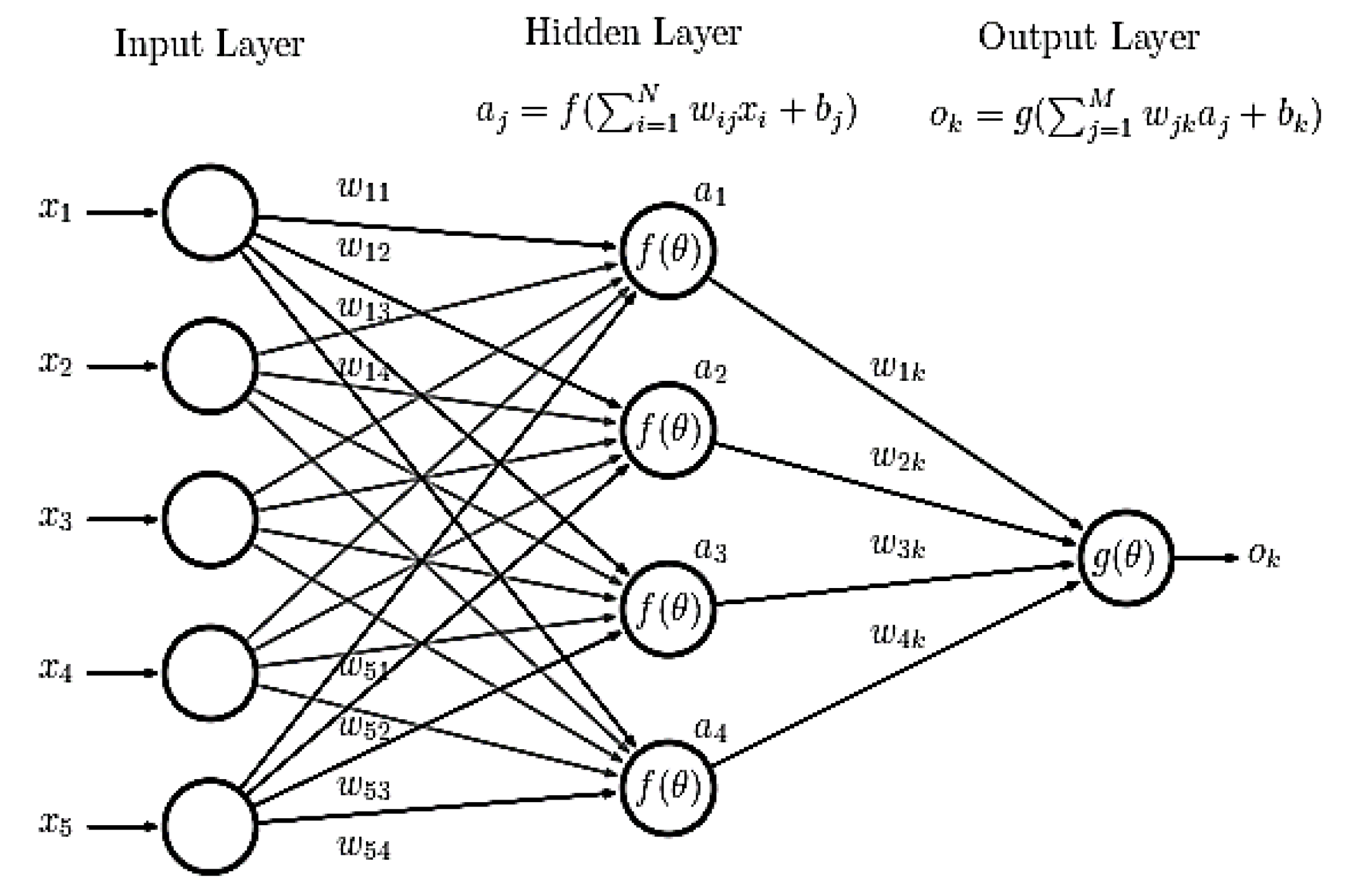
ANN is a branch of Artificial Intelligence (AI) made up of a varying number of neurons or nodes that can understand and establish any complex or non-liner relationship amongst inputs and outputs by using its interconnect neurons’ weights and bias matrices and transfer functions. These weights and bias are updated through learning so that the minimum error between the targets and desired outputs is achieved. This learning process is of two types, namely, supervised learning and unsupervised learning [12]. In supervised learning, a labelled data set is given for the network, and an answer key is used to compare with the network output, thus determining the accuracy of the network after training. In contrast, unsupervised learning uses unlabelled data set from where the algorithm extracts the features and patterns on its own. This study considers the supervised learning to train the network as the data are already categorised based on weather condition and water depth.

A visual illustration of this process is given in Figure 1. Five inputs in this figure are all relayed to four neurons in the first layer, known as the hidden layer, and then those four neurons will relay the final decisions to an output neuron. Depending on the complexity and the nature of data, the number of neurons and hidden layers is determined to minimize error after each learning stage.

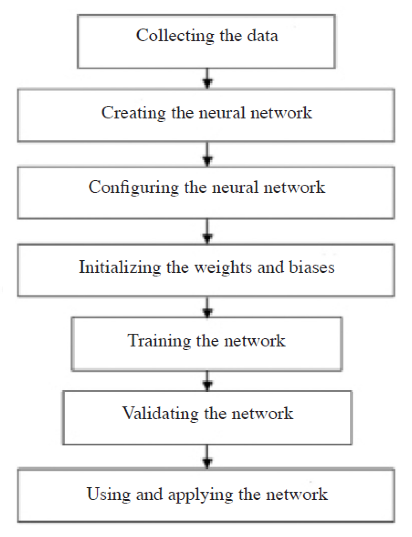
In this research, a feed-forward neural network is chosen with the backpropagation technique while training ANN. Beale et al. [13] and Hagan et al. [14] described the design steps of neural networks in the Neural Network Tool Box User Guide. The study reported here also follows the same steps which are shown in Figure 2.

Training of an ANN plays a significant role in justifying its effectiveness. The accuracy of the prediction depends on how well it is trained. In this research, the training of the network is carried out using a feed-forward backpropagation algorithm. The network performs a two-phase data flow here. In the first phase, the input information is propagated from the input to the output layer. Then the errors calculated from the network predicted values and actual values are backpropagated from the output layer to the previous layers and then to update the weights and biases accordingly. These weights and biases are updated based on a gradient descent algorithm, where the network weights are moved along the negative of the gradient of the performance function. Each neuron in the constructed net acts as a processing element which performs a weighted sum of all the inputs fed to it. Then it is transferred to the other neurons in the adjacent layer through a non-linear transfer function.

In this study, the Matlab neural network toolbox is utilized for training. A training function based on the Lavenberg-Marquardt algorithm has been found to work best, and it uses the following approximation of the Hessian matrix in order to follow the Newton-like update.

$$x_{k+1}=x_k-{[J^{T}J+\mu I]}^{-1}{J}^{T}e$$

(1)

where J_m is the Jacobian matrix that contains first derivatives of the network errors with respect to the weights and biases, e is a vector of network errors, and μ is a scalar value. This algorithm facilitates faster training, and also offers higher accuracy in function approximation. In the case of the transfer function, log-sigmoid is found suitable, which is given as

$$f(x)=\frac{1}{1+e^{-x}}$$

(2)

and the performance of the trained network is judged depending on the calculated mean squared error value (MSE). If the normalized teaching data are considered in the following form:

$$\{p_1,q_1\},\{p_2,q_2\},\dots \dots \dots \{p_n,q_n\}$$

(3)

where p is the input of the network, and q is the target output. Therefore, MSE can be calculated as follows:

$$MSE=\frac{1}{n}{\displaystyle \sum _{i=1}^{n}e{(i)}^2}=\frac{1}{n}{\displaystyle \sum _{i=1}^n{(q(i)-O(i))}^2}$$

(4)

where, O is the output of the network.

Using the aforementioned strategies, networks are trained for different sets of input data, as described in Section 3.

2.6. Validating the Established ‘Decision Making’ Platform Using Field Data

After the decision-making platform is trained, it is validated against two recent projects undertaken by the vessel. The variable data for two projects, one DP and another SM are provided as input into the decision-making platform and the outcome is compared with the operator’s actual decision. More details on ANN training and validation are presented in the results and discussion section.

3. Results and Discussion

The results of training the ANN with all the relevant cost and time factors for both the DP and SM systems (as shown in Table 1) are described in this section. All these variables’ contributions are then converted into monetary values for ERN 0 for any water depths up to 150 m. After that, the ANN is trained to predict the overall operational cost for both the DP and SM systems for any particular operational scenario (wave, wind, current, water depth, project durations, etc.), becoming the decision-making platform. Finally, the developed model is validated against the real operational scenario by predicting the best station-keeping options for two recent projects undertaken by the vessel used in this research.

3.1. Overall Operational Cost for the DP System

Besides initial investment on the DP system, the operator incurs operational and maintenance costs while running the system. For example:

• Compliance—such as annual trials, five-yearly FMEA and classification survey;
• Equipment calibration—such as MRU and gyro compass require calibration at specified intervals;
• Subscription—Such as GPS, DGPS, GNSS and electronic charts;
• Crew competency—DPO for officers and DP maintenance course for Engineers;
• Equipment health check—by maker annually or intermediate;
• Spare parts;
• FO consumption;
• Additional crew.

All these cost components, except the FO consumption and additional crew costs, are included in the vessel’s day rate (the overhead cost to maintain the system), as these costs will be there regardless of the vessel working on the DP or SM system. The total amount for these costs will depend on the time spend in station-keeping. Hence, one needs to calculate the FO consumption and time spent in station-keeping while operating the DP system. After that, these two variables should be converted into costs by multiplying with appropriate values and summed up with additional crew costs to determine the total operational cost.

3.1.1. FO Consumption Cost

The FO consumption data were collected as an average of every four-hour interval from a computerized FO monitoring system onboard, as mentioned in Section 2.3. The tracking of FO consumption starts as soon as the vessel arrived at the project location and tracking continued until it left the location after completing the job. For a DP-assisted, stationkeeping vessel, the vessel’s positioning upon arrival is time-consuming and depends on weather conditions. However, demobilizing from the location is almost immediate.

The consumption data collected for various projects with vessels operating at different water depths are categorized according to the ERN (similar to sea state), as shown in

Table 3. FO consumption at various depth and ERN [for DP mode].

Water Depth (m)	FO Consumption (Kg) at 4 h Block
	ERN 2	ERN 3	ERN 4	ERN 5	ERN 6
20	2100	2139	2168	2177	2191
30	1928	1977	2020	2026	2050
40	1771	1824	1857	1868	1878
50	1674	1726	1758	1768	1791
55	1607	1652	1683	1694	1703
60	1598	1594	1625	1642	1649
75	1493	1540	1575	1584	1595
80	1460	1502	1537	1546	1552
85	1411	1449	1493	1504	1513
90	1372	1423	1464	1478	1490
95	1350	1397	1440	1449	1462
100	1356	1400	1429	1439	1455
110	1355	1393	1421	1427	1433
120	1355	1395	1421	1426	1437
130	1350	1399	1421	1427	1436
140	1349	1393	1421	1427	1435
150	1351	1391	1421	1428	1437

. About 80% of the data presented in this table is collected from the real operational scenario. The remaining 20% (highlighted in bold) is predicted by the ANN to complete the table. The main reason for missing data is that the vessel either did not work in that specific water depth or encounter the weather conditions for the specified ERN. Therefore, the ANN is trained with the available data, and then, the reaming missing data were predicted by the trained system.

Table 4. Characteristics of the trained ANN for FO consumption in DP system.

Parameters	Values
Input	2 (ERN and water depth)
Output	1 (FO consumption)
Hidden layers	2
Neurons	8.5
Iteration	59
MSE	9.67 × 10−6
Gradient	2.44 × 10−5

shows the details of the ANN used to learn the data of FO consumptions for the projects run with DP-assisted station-keeping.

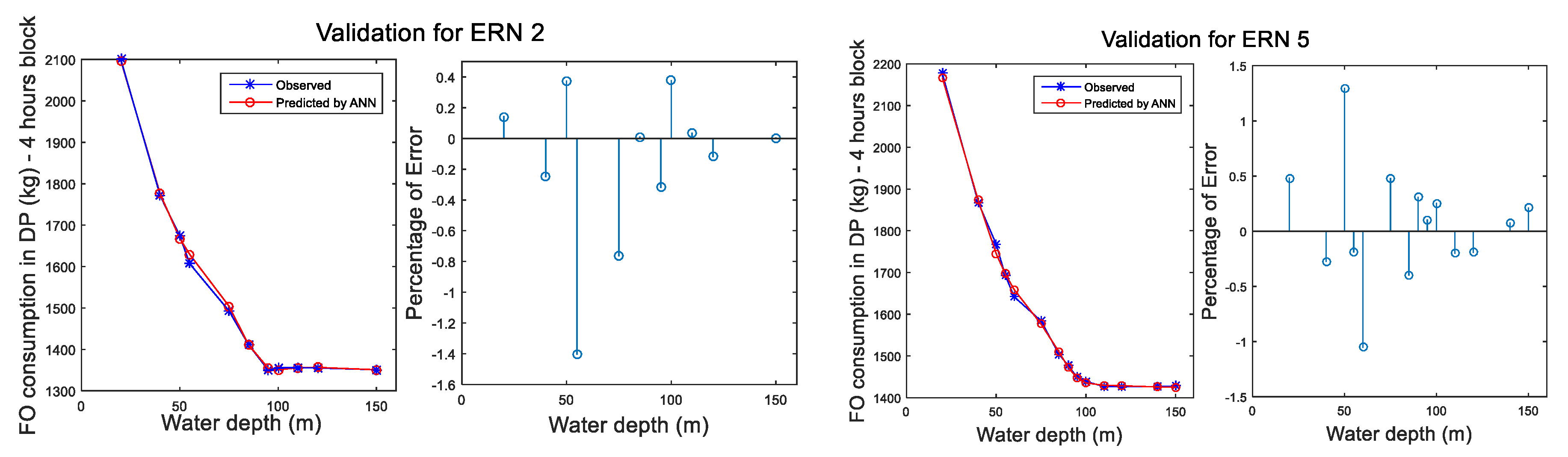
The trained network is validated for both trained and non-trained fuel consumption data. Figure 3 shows the comparison plots of ERN 2 and ERN 5 for the observed and ANN-predicted fuel consumption values. Generally, the FO consumption is reduced as the water depth increases and becomes steady after a certain depth. This is because the vessel requires more effort to generate the desired thrust in reduced water quantity. The water might also mix with mud and sand in shallow water, making the water density heavier. As can be seen in Figure 3, both the plots exhibit similar trends. The figure also includes the percentage of error for the data after learning, which is within 1.5%. All these comparisons demonstrate good predictability of the trained ANN tool, which is then utilized to predict the unknown data (highlighted in bold in Table 3) at various water depths.

The trained ANN is then further utilized to predict the fuel consumption values at various depths when there is no environmental force, which is ERN zero. Figure 4 shows a graphical plot for the ANN-predicted fuel consumption values for ERN 0 condition. The predicted values are for 4 h block, and as can be seen, the consumption is reduced with the increase in water depth and finally reaches a steady-state, as expected. Therefore, for daily consumption, the values are multiplied by six for cost calculation.

Now, to obtain the total cost for FO consumption (Y₁), these four-hourly fuel consumption values are multiplied by six to get the daily consumption, which later is multiplied by the per-unit FO price and the number of days of operation. This can be expressed by the following equation:

$$\begin{gathered} Y_1=ANN predicted FO consumption for DP\times 6\times FO price \\ \times Number of days of fieldwork \end{gathered}$$

(5)

3.1.2. Additional Crew Cost for DP Operation

Generally, most geotechnical survey vessels are manned by three deck officers and the Captain on deck department, and three engineers and the Chief Engineer on the engine department. The deck officers and engineers will perform four hours of keeping watch, followed by eight hours of rest during daytime and night-time. During their rest hours or watch hours, the officers and engineers must also perform other duties and responsibilities assigned to them besides keeping watch, while meeting MLC rest hour requirements.

The geotechnical vessel can comply with the above manning force requirements when operating in the SM system. However, for the DP operation, the above manning level is not enough as the engine room and navigation bridge are required to be manned by at least two engineers and two officers, respectively [15]. According to IMCA guidelines, the navigation bridge is required to be manned by one DPO and one SDPO. The DPO and SDPO are responsible for monitoring the vessel position, the performance of the DP system, and intervening in the DP system, when necessary [16].

Therefore, additional DPO and engineer are required to assign to the vessel whenever the vessel is planned to operate in the DP system. Since the vessel under consideration is operating in APAC, additional crews are assumed to be from the Philippines or Indonesia, and their contract is at least for a month with 2-week options.

The following costs are usually anticipated for these additional manning requirements:

• Crew remuneration (day rate);
• Mobilisation and demobilisation cost.

The latter includes flight cost, accommodation, local transport, sign-on/off cost and agency cost. Therefore, the total cost for additional crew for DP operation (Y₂) can be represented by the following equation:

$$Y_2=2\left[c+\frac{d}{30}\right]\times \mathrm{Number}\mathrm{of}\mathrm{days}\mathrm{of}\mathrm{fieldwork}$$

(6)

3.1.3. Time Factor Cost in DP Operation

This cost is calculated by finding the total days of DP operation (including positioning and duration of fieldwork) and multiplying it by daily OPEX. The time data are collected in minutes based on the records available in the vessel’s logbook. The time taken for DP positioning is mainly contributed by the vessel machinery type, crew competency and environmental condition. As explained in Section 2.3, the machinery type and crew competency are not considered in this study, while the weather condition is assumed to directly affect the time required for the vessel’s final positioning. Therefore, the time taken to position the vessel for various projects and different water depths is collected and arranged according to ERN, mostly ERN 2 to 4. It is standard operating practice that commencing any DP operation in ERN 5 and above shall be avoided. Hence, no positioning data for ERN 5 and above are found. The values are shown in

Table 5. Time taken for DP system positioning at various depth and ERN.

Water Depth (m)	Time Taken for DP Setup (minutes)
	ERN 2	ERN 3	ERN 4
20	55	65	85
30	51	63	83
40	50	65	80
50	50	60	80
55	45	60	75
60	45	55	75
75	45	55	75
80	42	50	73
85	40	50	70
90	40	50	65
95	40	50	65
100	40	45	60
110	40	45	60
120	40	45	55
130	40	46	58
140	40	45	55
150	40	45	55

. Similar to FO consumption data, unavailable DP positioning data are calculated using ANN and bolded in Table 5. It should be noted here that demobilizing the vessel from the position after completing the project in DP mode is almost immediate; hence, the time duration in this regard is neglected in the calculations.

A similar configuration of ANN as to FO consumption prediction has been used for training the network with the collected time data for the DP set up as well.

Table 6. Parameters of the trained ANN for the time taken to set up the DP.

Parameters	Values
Input	2 (ERN number and water depth)
Output	1 (Time)
Hidden layers	2
Neurons	12.8
Iteration	96
MSE	5.03 × 10−5
Gradient	0.00259

shows the details of the ANN used to learn the data in this regard.

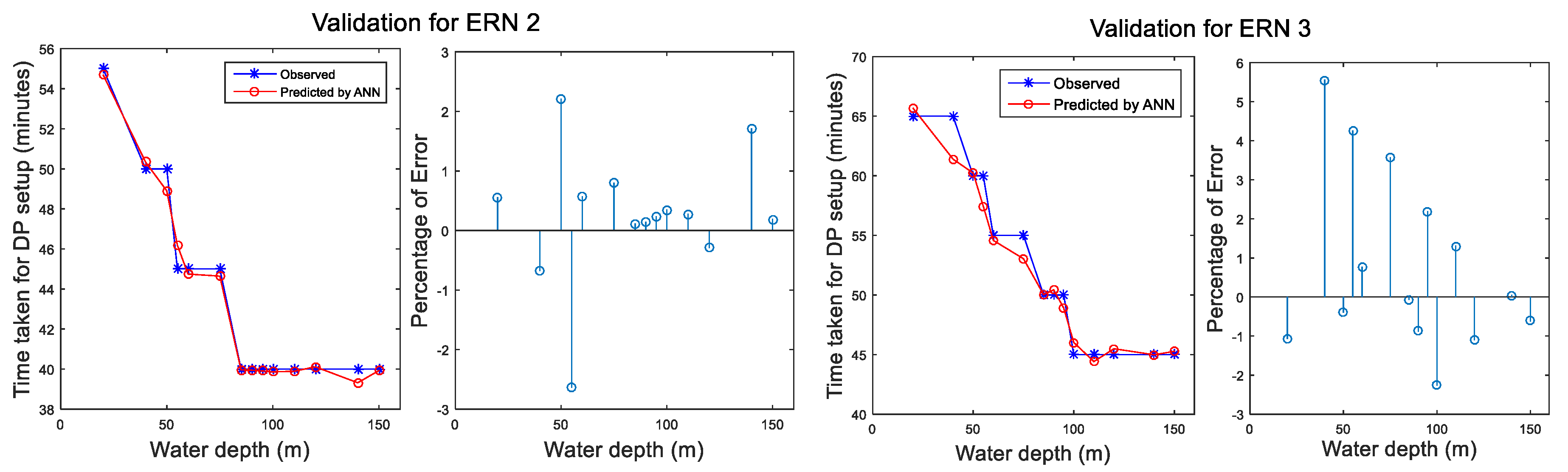
This trained network is also validated for both the trained and non-trained data for the DP set-up time. Figure 5 shows the comparison plots of ERN 2 and ERN 3 for the observed and ANN predicted data. The percentage of errors for the data after learning is within 5.5% limit. From the plot, we can conclude that the vessel requires a longer time to position in shallow water. For each ERN number, after reaching a certain depth, the time required to position the vessel is no longer influenced by water depth. For ERN 2, the time required to position the vessel at the water depth of 85 m and beyond remains at 40 min. While, for ERN 3, the time required to position the vessel at the water depth of 100 m and beyond remains at 45 min. These conclusions are agreeable with the data presented in Table 5. The trained ANN is then utilized to predict the unknown data in Table 5 at different water depths.

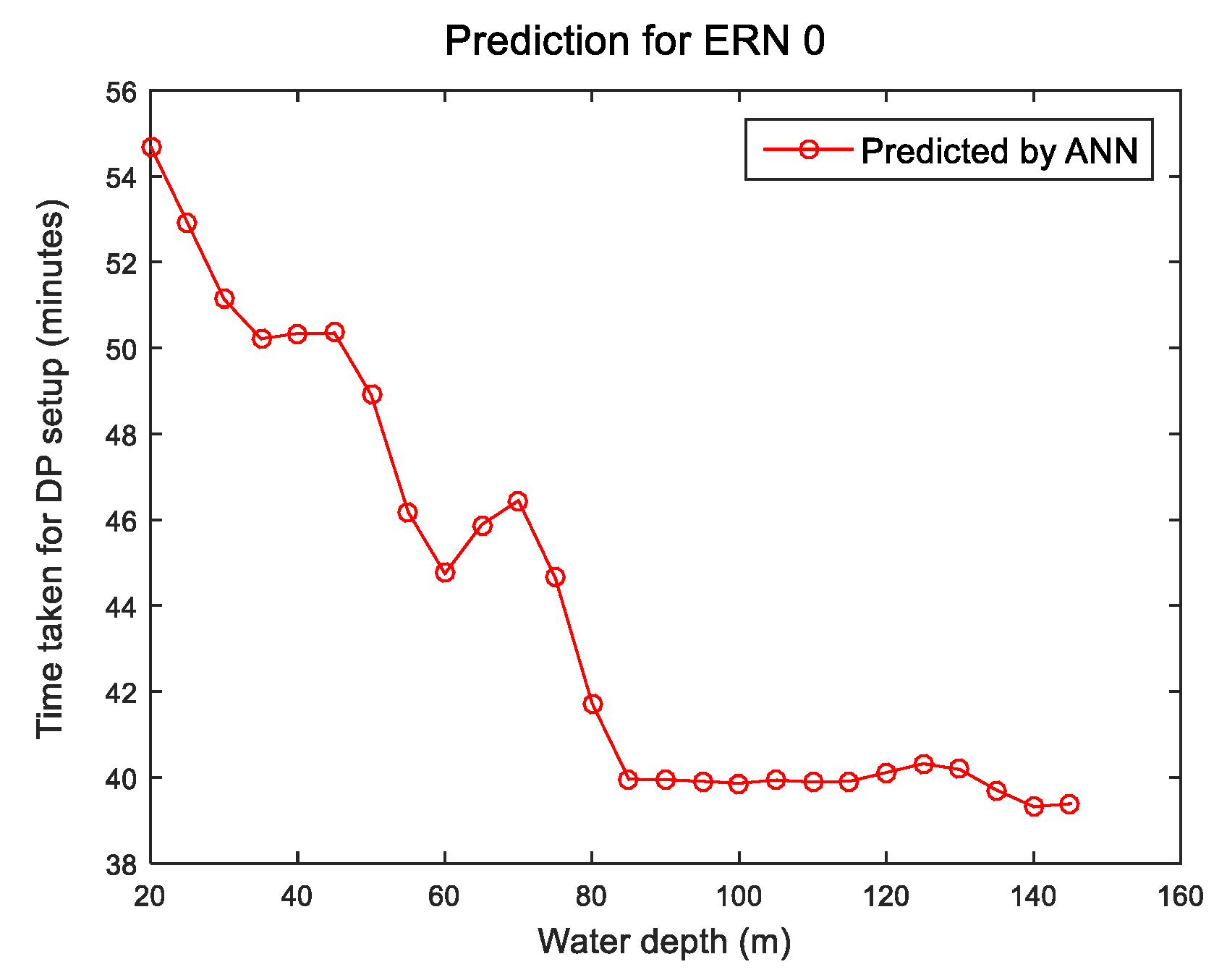
The trained ANN is further applied to predict the time taken for DP set up at various water depths when there is no environmental force (ERN zero). Figure 6 shows a graphical plot for those ANN-predicted time at ERN zero conditions for various water depths. As can be seen, time saturation occurs at water depth 85 m, and beyond that, the time remains constant at 40 min.

Once the above formulation is done, the total cost for time factors (Y_s) can be calculated using the following equation:

$$Y_3=\left(\frac{\begin{array}{c}ANN predicted time for\\ DP Setup \left(minute\right)\end{array}}{24\times 60}\right)\times Field work duration\left(days\right)\times daily OPEX$$

(7)

3.2. Overall Operational Cost for the SM System

Similar to Section 3.1, the overall operational cost for the SM system is calculated in this section. Unlike the DP system, there is no cost element for extra crews in SM operation. Hence, only the FO consumption and time spend in station-keeping while operating in the SM system is needed to be calculated. After that, these two variables should be converted into cost by multiplying with appropriate values and summed up to determine the total operational cost.

3.2.1. FO Consumption Cost

When the vessel is operating on SM, the FO consumption is purely driven by demand in hotel services and drilling equipment. However, positioning and de-positioning the vessel in the desired location in SM is complicated compared to DP. These are time-consuming processes that will cause additional FO consumptions. Usually, the positioning takes more time and consume more FO compared to de-positioning. Two azimuth thrusters and two bow thrusters are required during deployment and retrieval of the spread mooring anchors. So, two main engines and two shaft generators will be in operation. The operation can either be performed by manual steering, which completely depends on the operator’s competency or the DP system.

Once the positioning is completed, unlike DP, the station-keeping FO consumption for SM will not depend on ERN nor much on water depth. Therefore, considering all these facts, the data for FO consumption for various SM operated projects at various water depth is collected in three separate regimes:

During positioning (at various ERN): manoeuvring, dropping anchors, pulling and positioning.

Stations keeping by SM (ERN ignored as not much influence): only two auxiliary engines are running.

During de-positioning (at various ERN): pulling and picking up anchors by the winch; minimum propulsion.

Table 7. FO consumption in SM for various ERN and water depths.

Water Depth (m)	Positioning (Total FO Consumption in KG)			Station Keeping (Daily Average FO Consumption in KG	(Total FO Consumption in KG)
	ERN 2	ERN 3	ERN 4		ERN 2	ERN 3	ERN 4
20	630	665	700	3800	350	350	420
30	805	805	840	3810	385	420	490
40	926	890	948	3805	428	472	542
50	1071	1120	1165	3800	470	490	580
55	1225	1260	1295	3785	490	525	595
60	1323	1328	1413	3800	504	540	610
75	1622	1505	1575	3815	539	595	665
80	1610	1645	1701	3825	560	630	700
85	1715	1750	1820	3800	595	665	735
90	1880	1884	1899	3800	630	703	783
95	1955	1960	2012	3800	658	735	832
100	2030	2100	2170	3810	679	770	875
110	2137	2251	2343	3813	707	816	935
120	2240	2310	2401	3815	735	805	966
130	2337	2514	2543	3803	779	879	995
140	2450	2541	2625	3790	840	924	1050
150	2590	2660	2765	3800	910	980	1120

shows the collected FO consumption data for the above three situations. It is a standard operating practice that commencing positioning and de-positioning of the vessel in weather conditions ERN 5 and above shall be avoided. Therefore, data are available only for ERN 2 to 4. In addition, as mentioned earlier, the daily average FO consumption for station-keeping is not influenced by the weather condition once the vessel is fully in position. A small fluctuation in daily FO consumption is observed, which is mainly caused by high starting current and variation of power demand in hotel services and drilling equipment. Therefore, the FO consumption during station-keeping in spread mooring is considered as a daily average value. Under the station-keeping FO consumption column, Table 7 shows those average daily FO consumption values.

It should be noted here that about 70% of the data in this table are actual values collected from the vessel’s log, while the remaining 30% (highlighted in bold) are predicted based on the trained ANN. Similar feed-forward ANNs applied in earlier sections are trained and used to predict FO consumption while positioning and de-positioning the vessel in SM system.

Table 8. Parameters of the trained ANNs for FO consumption prediction in SM system.

Parameters	Positioning	De-Positioning
Input	2 (ERN number and water depth)	2 (ERN number and water depth)
Output	1 (FO consumption)	1 (FO consumption)
Hidden layers	2	2
Neurons	10.5	10.5
Iteration	80	26
MSE	1.32 × 10−12	1.67 × 10−14
Gradient	1.7 × 10−6	1.73 × 10−9

shows the details of the ANNs used in this regard.

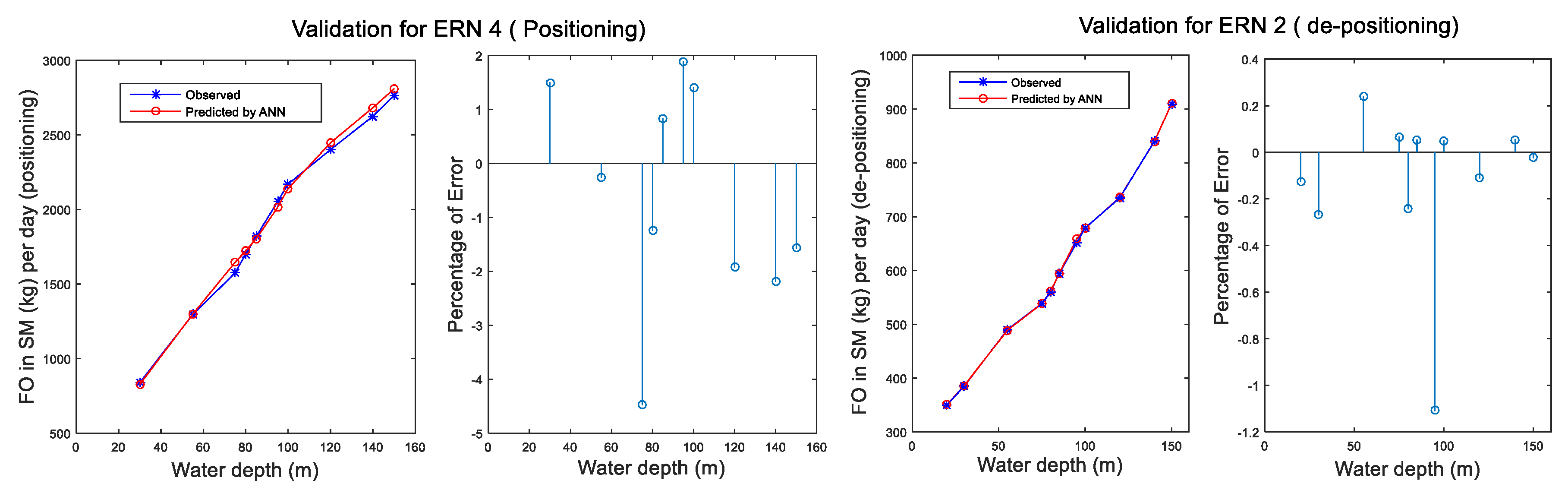
Figure 7 depicts the comparison plots at ERN 4 (positioning), and ERN 2 (de-positioning) for both the observed and ANN predicted FO consumption values for the SM system. The percentage of error for the data after learning is within 5%.

The ANNs are then used to predict the FO consumption for the SM system in various depths for ERN 0. Figure 8 shows the predicted values for both positioning and de-positioning.

The total cost for FO consumption for spread mooring operation (Y₄) can now be obtained by using the following equation:

$$\begin{array}{c}{Y}_4=(ANN predicted FO consumption for positioning+\\ ANN predicted FO consumption for depositoning\\ +3804\times number of days of field work)\end{array}$$

(8)

3.2.2. FO Consumption Cost

Similar to the DP operation, the cost here is calculated by finding the total days of SM operation (including positioning, de-positioning and duration of fieldwork) and multiplying it by daily OPEX. The time data are collected in minutes based on the records available in the vessel’s logbook. The factors that influence the setup and removal time for SM operations are:

Water depth: as water depth increases, the required wire length will increase.

Weather: As the ERN number increase, more wire is required on the seabed to withstand the force. Deployment and retrieval will take more time with an increase in FO consumption.

Mooring footprint: sometimes, a larger footprint is required to perform drilling in more than one location, which falls within the mooring footprint. This factor, however, is not considered in this study.

As can be seen, both the water depth and weather conditions directly affect the time required for the vessel’s final positioning and de-positioning. Therefore, the time taken for these two activities for various projects at different water depths is collected and arranged for ERN 2 to 4, as depicted in

Table 9. Time taken for SM system positioning and de-positioning at various depth and ERN.

Water Depth (m)	Positioning (Time Taken, min)			De-Positioning (Time Taken, min)
	ERN 2	ERN 3	ERN 4	ERN 2	ERN 3	ERN 4
20	90	95	100	50	50	60
30	115	115	120	55	60	70
40	145	138	147	58	65	76
50	168	160	173	60	70	82
55	175	180	185	70	75	85
60	182	187	194	73	78	88
75	213	215	225	74	85	95
80	230	235	243	80	90	100
85	245	250	260	85	95	105
90	261	266	289	90	102	111
95	275	280	296	94	105	118
100	290	300	310	97	110	125
110	303	317	328	102	113	133
120	320	330	343	105	115	138
130	335	344	355	108	121	142
140	350	363	375	120	132	150
150	370	380	395	130	140	160

. Similar to FO consumption data, unavailable SM positioning, de-positioning data are calculated using ANN, and those predicted data are bolded in Table 9.

A similar configuration of ANN as to FO consumption prediction has been used for training the network with the collected time data for the SM set up as well.

Table 10. Parameters of the trained ANN for the time taken to set up and remove the SM system.

Parameters	Positioning	De-Positioning
Input	2 (ERN number and water depth)	2 (ERN number and water depth)
Output	1 (Time taken)	1 (Time taken)
Hidden layers	2	2
Neurons	10.5	10.5
Iteration	80	26
MSE	1.32 × 10−12	1.67 × 10−14
Gradient	1.7 × 10−6	1.73 × 10−9

shows the details of the ANN used to learn the data in this regard.

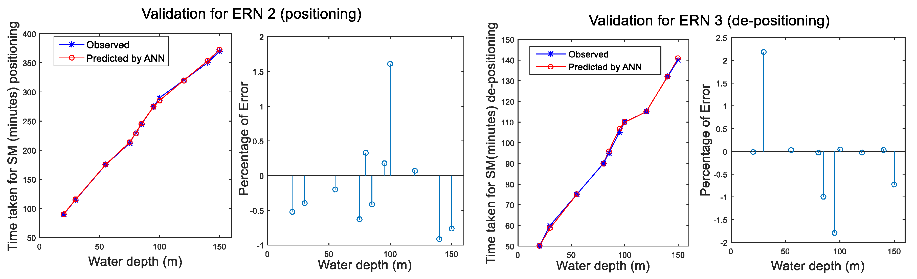
This trained network is validated for both the trained and non-trained data for SM set up and removing time, and Figure 9 shows the comparison plots of ERN 2 (positioning) and ERN 3 (de-positioning) in this regard where the amount of error is less than 2%.

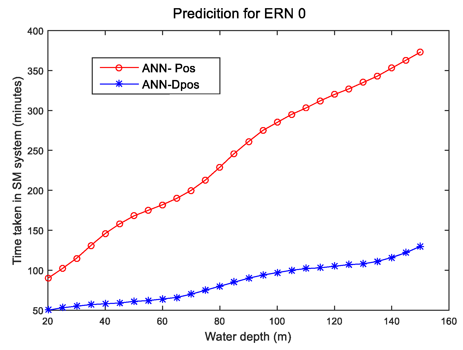
The trained ANN is further applied to predict the time taken for SM positioning and de-positioning at various water depths when there is no environmental force (ERN zero). Figure 10 shows a graphical plot for those ANN-predicted times at ERN zero conditions for various water depths. As noticed, the time increases with the increase in water depth, which is expected as longer mooring length is required.

The predicted values are then used to calculate the associated time costs (total cost for vessel keeping) for the SM system, using the formula in Equation (9).

$$Y_5=\left(\frac{ANN predicted time for positioning+ANN predicted time for depositioning}{24\times 60+Number of days of field work}\right)$$

(9)

3.3. Demonstration of the Decision-Making Capability of the Trained ANNs

The accuracy of the decision making of the trained ANNs is validated against two recent actual projects undertaken by the vessel, one for SM and another for DP. Before presenting the validation results, the rationale of decision making is explained in the following subsection.

3.3.1. The Rationale behind Decision Making

As described in the earlier section, the study of decision making reported here is solely based on cost estimation. The trained ANN will estimate the total operational cost based on the information made available and decide which option (DP or SM) provides the lower cost for that particular scenario. Using the equations developed in Section 3.1 and Section 3.2 the total costs for DP and SM operation for any operational scenarios can be estimated by Equations (10) and (11), respectively.

$$Cos{t}_{DP}=Y_1+Y_2+Y_3$$

(10)

$$Cos{t}_{SM}=Y_4+Y_5$$

(11)

Both these equations contain several variables those changes depending on market condition, thus, will affect the total cost significantly. For the analysis presented in this subsection, the following values are considered for some of those variables:

• Vessel’s daily OPEX—USD 30,000
• Estimated days of fieldwork based on scope—variable
• Water depth—variable
• FO price (Marine clean MGO, sulphur <0.05%)—USD 500/tonne or USD 0.5/KG
• Daily rate for additional crew for DP operation—USD 300
• Monthly virtualization cost for DP crew—USD 2500

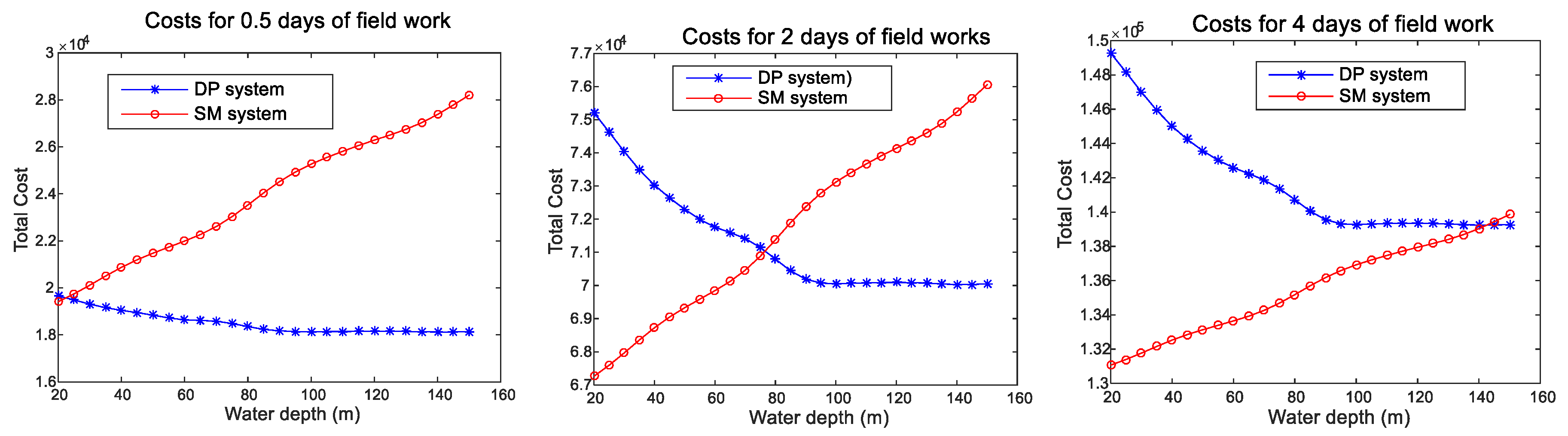
Now, considering three different durations of fieldwork, the cost of DP and SM operations at various water depths is estimated and plotted in Figure 11 for ERN 0. The three plots depict the dynamics of decision making involved in this process. For example, as can be seen, when the fieldwork is limited to 0.5 days, the DP system is always cheaper if the water depth is above 22.5 m. On the other hand, for 2 days of fieldwork, SM remains cheaper as long as the water depth is within 75 m. The threshold value of water depth shifts further right with the increase in fieldwork duration.

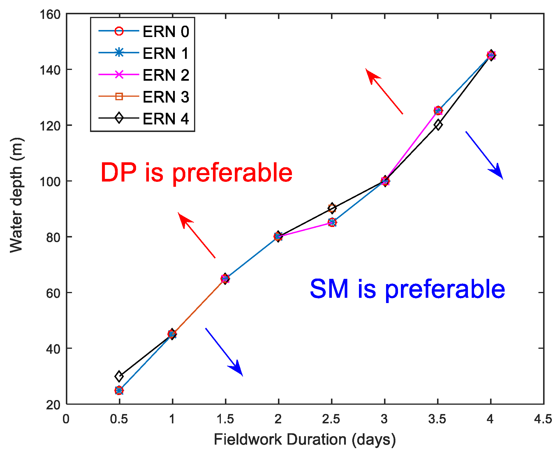
Although the results plotted in Figure 11 are for ERN 0 only, similar trends are observed for other ERNs as well. Therefore, to understand the dynamics in decision making for different ERN numbers and see how the threshold water depth varies with the change of fieldwork duration, Figure 12 is plotted. The figure represents five decision-making boundaries that separate the preferred operational zones for DP and SM based on ERNs, water depths and fieldwork durations for the particular set of cost variables considered here. As can be seen, the threshold water depth is almost constant for various ERNs for this particular operational scenario. The ANN will generate different sets of decision-making boundaries once the variables keep changing. Therefore, this plot could deliberately be used as a guideline for instant decision making for any geotechnical vessel on whether DP or SM will be the best choice for a given operational scenario.

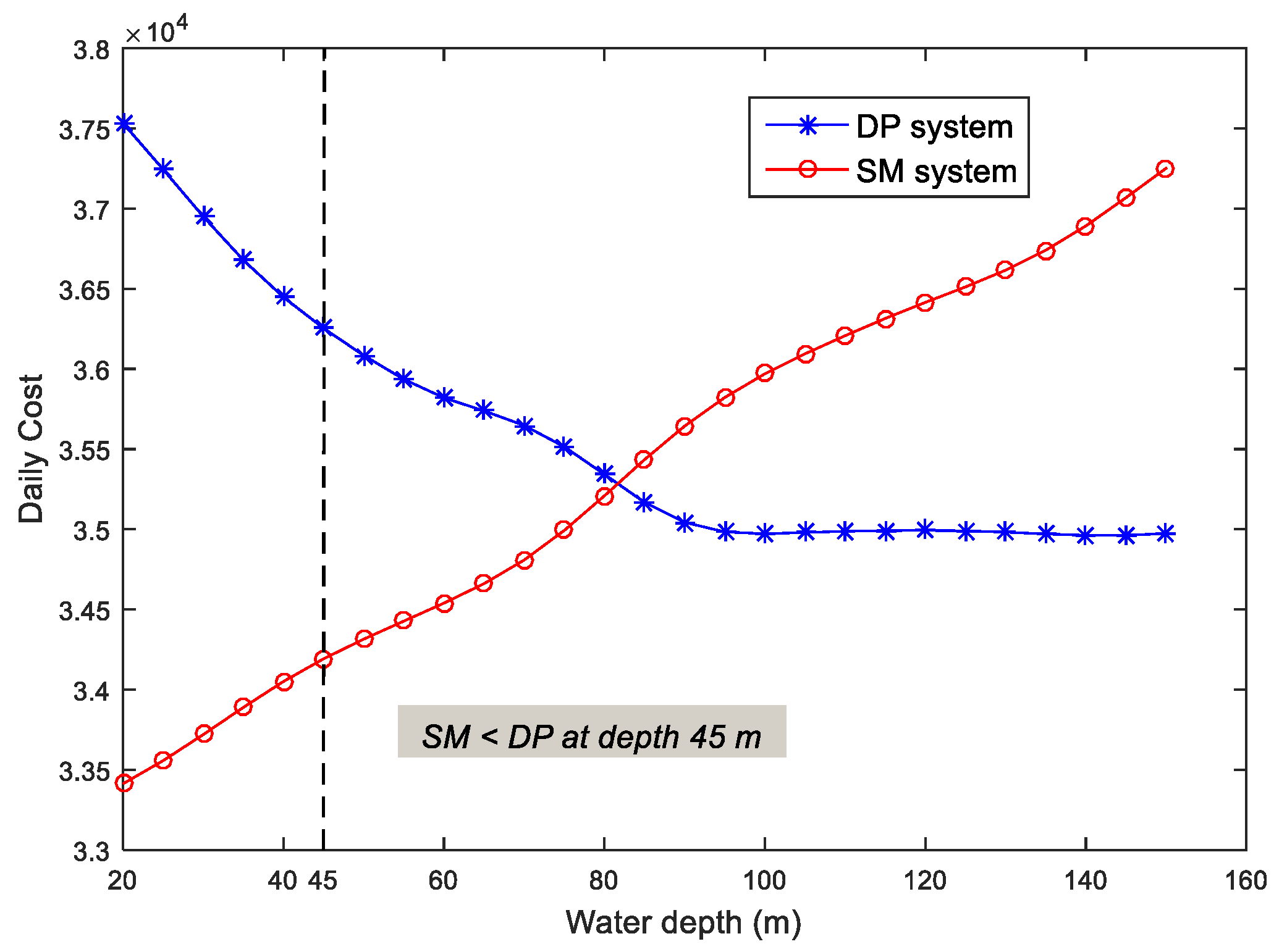
3.3.2. ANNs Validation against SM Scenario

Table 11. Specification for a project undertaken with SM arrangement.

Project Location	Offshore Brunei
Client	Confidential information
Overall Scope	Marine site characterisations for 3 Jack up rig emplacement.
Location	Confidential information
Scope on location	1 × 30 m CPT sampling; 1 × 45 m continuous PCPT hole; 1 × 60 m continuous sampling borehole.
Water Depth	45 m (Chart Datum)
Duration at location	55 h (2.29 days) on 10 March 2020 to 13 March 2020
Station Keeping mode	Spread Mooring (Four Point Mooring—self-anchoring)

shows the information on a recent project undertaken by the drilling vessel considered in this study. The project was completed using the SM arrangement. Now, the trained ANN is fed with variable values specific to this project (FO cost, crew costs etc.), and is allowed to generate plots for overall project costs for the operation of 55 h, using both DP and SM arrangement, and for various water depths. Figure 13 shows the results, where the vertical dotted line indicates the operational water depth at the project site. As can be seen, the ANNs concluded that SM is cheaper than DP at 45m water depth for a project duration of 2.29 days (55 h), which matches with the actual mode of operation choose by the operator.

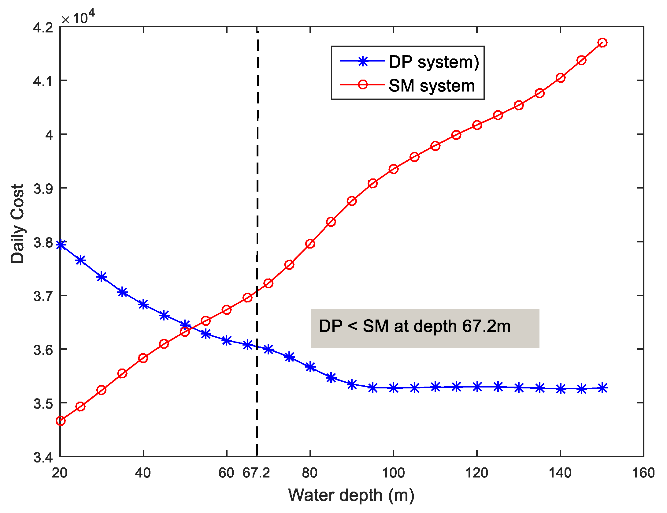
3.3.3. ANNs Validation against DP Scenario

The steps similar to Section 3.3.2 is repeated here except that this time it is for a different project with a duration of 1.25 days.

Table 12. Specification for a project undertaken with SM arrangement.

Project Location	Offshore Thailand
Client	Confidential information
Overall Scope	Marine site investigation on site suitability for platforms and jack-ups development at Chevron fields, Offshore Thailand.
Location	Confidential information
Scope on location	1 × 140 m sample boreholes (0 m to 15 m @ 1 m sampling interval; 15 m to 30 m @ 1.5 m sampling interval; more than 30 m @ 2 m sampling interval)
Water Depth	67.2 m (62.7 m echosounder + 4.5 m draft)
Duration at location	30 h (1.25 days) on 20 May 2020 to 21 May 2020
Station Keeping mode	DP 2

shows project specifications, and Figure 14 shows ANNs prediction on suitable station-keeping options based on total operational cost. As indicated by the vertical dotted line, it is evident that DP is cheaper than spread mooring for this particular project while the vessel operated at 67.2 m water depth for a duration of 1.25 days. This decision from ANNs also matches with the actual decision taken by the operator for this project.

4. Conclusions

A systematic study on developing an ANN-based decision-making model to make optimum station-keeping choice for a geotechnical drilling vessel is presented. To summarize:

• This research utilizes Artificial Neural Networks as a powerful learning tool constructed from data gathered from a geotechnical drilling ship to predict the operational cost and thereby, deciding on the best station-keeping option.
• Factors such as confidence level on the weather forecast, crew competency, and system readiness are ignored in the present modelling; however, these should be considered in the selection process to improve the ANN prediction.
• While the study reported here is specific to station-keeping of geotechnical drilling vessel, it can be easily extended for other Offshore Support Vessel operational scenarios.
• The optimization approach in station-keeping can further be developed by collecting data from more vessels with the same objective to increase the knowledge of ANNs. During station-keeping, the relationship between FO consumption in various weather conditions and the engine’s Specific Fuel Consumption (SFC) can be developed by applying a similar method.
• Proper decision-making in any marine application ensures better usage of resources and cost minimization and assists in achieving sustainable development while keeping the impact on the environment to a minimum. The concept presented in this study can be further applied in the development of a sustainable business model for the marketing of geotechnical drilling vessels and other similar ships.