Abstract
Though the ocean is sparsely populated by buoys that feature co-located instruments to measure surface winds and waves, their data is of vital importance. However, due to either minor instrumentation failure or maintenance, intermittency can be a problem for either variable. This paper attempts to mitigate the loss of valuable data from two opposite but equivalent perspectives: the conventional reconstruction of significant wave height (SWH) from Caribbean Sea buoy-observed surface wind speeds (WSP) and the inverse modeling of WSP from SWH using the long short-term memory (LSTM) network. In either direction, LSTM is strongly able to recreate either variable from its counterpart with the lowest correlation coefficient (r2) measured at 0.95, the highest root mean square error (RMSE) is 0.26 m/s for WSP, and 0.16 m for SWH. The highest mean absolute percentage errors (MAPE) for WSP and SWH are 1.22% and 5%, respectively. Additionally, in the event of complete instrument failure or the absence of a buoy in a specific area, the Simulating WAves Nearshore (SWAN) wave model is first validated and used to simulate mean and extreme SWH before, during, and after the passage of Hurricane Matthew (2016). Synthetic SWH is then fed to LSTM in a joint SWAN—LSTM model, and the corresponding WSP is reconstructed and compared with observations. Although the reconstruction is highly accurate (r2 > 0.9, RMSE < 1.3 m/s, MAPE < 0.8%), there remains great room for improvement in minimizing error and capturing high-frequency events.
1. Introduction
For an incredibly diverse range of coastal and open ocean studies, numerical model output, satellite data, and reanalysis products dominate the methodologies employed by researchers worldwide and are often used to supplement if not completely replace in situ platforms such as buoys. Nevertheless, in each case, before any of those methods could be reliably used, their robustness is nearly universally tested by their agreement with the same platforms [1,2,3,4,5]. A host of studies are naturally directly performed using buoy measurements [6,7,8,9], and thus, the fidelity and completeness of buoy measurements are of paramount importance as their data is extremely valuable. For small island developing states (SIDS) that possess neither the financial resources nor technical expertise to deploy and maintain large numbers of buoys, it is of even greater importance to fully use available buoy observations and to find methods to convert those observations into additional variables of interest.
As long shown by ocean remote sensing, the indirect derivation of parameters of interest from direct observations of another is a common problem. For example, a host of algorithms have been proposed to inversely model wind speed (WSP) from high-frequency coastal radar measurements [10,11,12] and Synthetic Aperture Radar (SAR) estimation of WSP from sea surface roughness [13,14]. Relevant to the current discussion, identical trends are identified for in situ observations, where recently, artificial intelligence and machine learning techniques have been widely employed and applied in WSP inversions from wave measurements. Daga and Deo attempted to derive WSP from wave measurements at five buoy locations through inverse modeling by using genetic programming (GP), model trees (MT), and a locally weighted projection regression [15]. Among the three methods, GP was found to be the most suitable in most cases. In a similar study, Kambekar and Deo used two data-driven models, GP, and MT to simulate and forecast waves using WSP at eight different buoys and found that while both methods performed satisfactorily, MT estimated higher waves more accurately [16]. Nitsure et al. used wind information ingested by GP to forecast wave heights at varying temporal horizons and found that the model accurately captured wave heights, even during hurricanes [17]. Charhate et al. compared GP and an ANN in the inverse modeling of deriving wind parameters from wave information and found that GP produced more accurate results [18]. Although Akbarifard and Radmanesh primarily used a symbiotic organisms search (SOS) algorithm to predict wave height in hourly and daily time ranges and compared its efficacy with other algorithms, they found that, crucially, coupling SOS with Simulating WAves Nearshore (SWAN) numerical wave model could be applied in areas of insufficient observations [19]. James et al. compared a trained multi-layer perceptron (MLP) model with SWAN output of wave height and wave period and found that the MLP could produce similarly accurate wave conditions as SWAN could but additionally could be run over 4000× faster [20]. Vieira et al. used an artificial neural network (ANN) to fill gaps in buoy data using publicly available wind and wave information generated from a numerical model-generated hindcast, demonstrating ANNs were viable alternative methods to wave modeling to fill gaps [21]. Widely used in oceanographic studies, the long short-term memory (LSTM) recurrent neural network has been applied primarily to forecast significant wave height. For example, Ni and Ma [22] used LSTM and Principal Component Analysis (PCA)-identified parameters to predict wave height from four buoys in the polar westerlies. Pushpam and Enigo used LSTM trained on three years of buoy data to perform 3, 6, 12, and 24 h significant wave height predictions [23]. Fan et al. also used LSTM in significant wave height predictions and additionally found that when SWAN was fed buoy-observed surface wind speed, the hybridized SWAN-LSTM model outperformed the single SWAN usage [24].
Considering the few buoys located throughout the Caribbean Sea, the value of their data is extremely valuable, especially at the onset of the United Decade of Ocean Science for Sustainable Development (2021–2030). Consequently, in this study, two fundamental observations made by buoys, surface winds and significant wave height, are converted from its counterpart through the usage of the LSTM network. In a case study, LSTM is coupled with SWAN and used to reconstruct mean and extreme (hurricane) wind speed from modelled significant wave height. The rest of the paper is structured as follows: Section 2 describes the data used and methodology employed. Section 3 provides the results. Section 4 gives the conclusion and a discussion.
2. Materials and Methods
2.1. In Situ Observations
Six Caribbean Sea-deployed buoys owned, operated, and maintained by the National Buoy Data Center (NDBC) were accessed for significant wave height observations for 2016 (Figure 1, Table 1). This year was chosen because each buoy had sufficient information to perform the required analyses. Data curating was performed to ensure a uniform hourly resolution of equal-length, contemporaneous wind, and wave data in each buoy because LSTM is unable to handle any gaps. In the case of NDBC buoy 42057 that only had 50% of observations (ranging from 1 January to 30 June 2016), invalid entries were removed, and the time series that remained was used to train the LSTM network. For all other buoys that had minor invalid entries distributed throughout the length of their time series, these were simply removed alongside the corresponding variable for that time step.
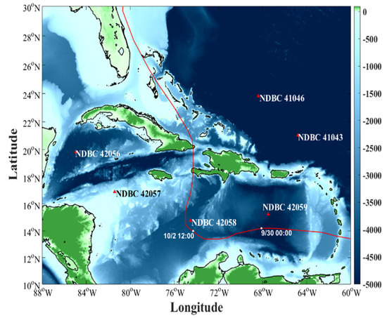
Figure 1.
The model domain, Hurricane Matthew (2016) best track (red line), and topography (shading, m) with utilized NDBC buoy positions marked (red triangles). The dates at which Matthew passes the nearest buoys are also marked.

Table 1.
NDBC buoy data statistics for 2016.
2.2. Numerical Model Configuration
Based on the spectral action balance equation, the phase averaged, third-generation wind-wave model Simulating WAves Nearshore (SWAN) version 41.10 [25,26] is employed to perform the wave simulations. The model is efficient at simulating wind-induced wave growth, energy dissipation due to whitecapping, bottom friction, and wave breaking, in addition to the nonlinear triad and quad interactions. In Cartesian coordinates, the governing equation is given as follows:
where σ is the radian frequency as observed in a reference frame moving along with a current velocity; N is the wave action density and is equal to the energy density divided by the relative frequency (N = E/σ); θ is the wave propagation direction; c is the wave action propagation velocities in x, y, σ, and θ space. Stot is the non-conserved source/sink term expressed as the wave energy density, which represents all physical processes that generate, dissipate, or redistribute wave energy and is given as:
where is wind-induced energy input; and are the triplet and quadruplet wave-wave interactions, respectively; is dissipation due to whitecapping; is dissipation due depth-induced wave breaking; is the dissipation by bottom friction. The transfer of wind energy input to waves is described by the resonance [27] and feedback [28] mechanisms; both linear and exponential wind input growth functions are included in the model. Whitecapping formulations based on a pulse-based model [29], as adapted by the Wave Model Development and Implementation (WAMDI) Group, are employed [30]. The selected bottom friction models are the Joint North Sea Wave Project (JONSWAP) [31] empirical model with a friction coefficient of 0.067 m2/m3, the drag law model of Collins [32], and the eddy-viscosity model of Madsen et al. [33]. Energy dissipation in random waves due to depth-induced wave breaking is dealt with by the bore-based model of Battjes and Janssen [34]. Deep and shallow water quadruplet and triad-wave interactions are activated using Discrete Interaction Approximation (DIA) default settings [35] and the Lumped Triad Approximation (LTA). Partially modeled diffraction is added to the model using a phase-decoupled refraction/diffraction method [36]. Through prior experimentation, it was found that the Janssen physics processes [37] produced the best results and are thus employed. SWAN model parameters and configurations are given in Table 2.

Table 2.
Simulating WAves Nearshore model configuration.
The model is implemented using an unsteady two-dimensional calculation mode and is on a spherical coordinate system for the geographical area enclosed by 60–88° W, 10–30° N. Bathymetric data is obtained from the General Bathymetric Chart of the Oceans (GEBCO; GEBCO_2014 Grid, http://www.gebco.net; accessed on 23 February 2021).
SWAN is forced with 6-h Climate Forecast System Reanalysis (CFSR) wind fields provided by the National Centers for Environmental Prediction (NCEP) reanalysis data on a spatial resolution of ~0.2° in both directions for September and October 2016. For clarification, the CFSR wind field is used only for driving the wave model and is not included in any subsequent assessments.
Although the Caribbean Sea is semi-enclosed, the Atlantic Ocean boundaries are naturally open and necessitate energy input to the model domain. Hourly WaveWatch III output developed at NOAA/NCEWP [38] was used as initial and boundary conditions. A spin-up time of two days was given before data is recorded on the first day of each of the two months. The data were recorded at computational grid points corresponding to the geographical locations of NDBC buoys 42058 and 42059 every 1 h.
2.3. The Long Short-Term Memory Network
Belonging to a class of artificial recurrent neural networks (RNNs), the long short-term memory was specifically developed to deal with the vanishing gradient problem and is highly efficient at data time series analysis [23,39]. Particularly, LSTMs have an advantage over conventional feed-forward neural networks and other RNNs in that they can selectively remember patterns in data for long durations, and this is accomplished by a series of forget (), input (), and output () gates, in addition to the sigmoid function () and Hadamard () product operator [40]. Each gate of the cell state may be computed as follows:
where W is each layer’s assigned weight; is the input time step t; b is the bias; tanh is a hyperbolic tangent function. As the name implies, the forget gate is used to forget past information, with decisions on which information to forget defined as the value obtained by taking the sigmoid following receiving and . The output of the sigmoid function ranges from 0 to 1 so that if the value is 0, the information of the previous state is completely forgotten, and if 1, the information is completely retained. Current information is saved in the input gate , where it takes the values of and and applies it to the sigmoid function. Following this, the value computed with the tanh function and Hadamard product operator is sent from the input gate. To represent the strength and direction of the current information storage, ranges from 0 to 1, and ranges from −1 to 1, respectively. The LSTM network will be used to perform both the conventional (wind-to-wave; the input is wind speed, and output is significant wave height) and inverse (wave-to-wind; the input is the significant wave height, and the output is wind speed) modeling of WSP and SWH from its counterpart variable. The LSTM cell state architecture is given in Figure 2.
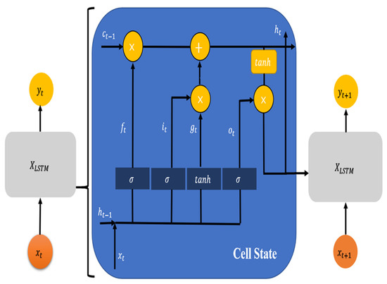
Figure 2.
The architecture of the long short-term memory (LSTM) cell state (‘X’), where xt and yt are the target variables before and after passing through the network at the current gate, respectively; xt+1 and yt+1 are the target before and after passing through the network at the next iteration, respectively.
The LSTM network is set up with four layers that correspond to a time step of 4. This time step was chosen as it falls within the forecast limit of 1–6 h for one year of training data as established by Fan et al. [24]. The recursive linear unit (relu) was used as the activation function to maximize the model’s ability to capture nonlinearities. The number of epochs was set to 50, and the batch size was set to 1. Partitioning of training and validation sets occurred at a 70/30 split. The training/testing split specifies the quantity of data used to train the model before the accuracy of the predictions is tested during model training. Throughout each experiment, operating parameters were held constant.
2.4. Performance Indicators
To evaluate model performance at variable reconstruction, three commonly applied statistical techniques to measure discrepancies between synthetic and observed values. The correlation coefficient (r2), root mean square error (RMSE) and mean absolute percentage error (MAPE) are given as follows:
where and are the observed and reconstructed variables, respectively.
3. Results
3.1. Conventional Modeling
In this first section, the conventional transformation of surface wind speed (WSP) into significant wave height (SWH) is performed. In Figure 3, with corresponding error statistics collated in Table 3, it can be shown that there exists a strong agreement between the synthetic and observed SWH. Specifically, an r2 of 0.99, an RMSE of 0.09 m, and a MAPE of 0.05 was returned for buoy 42056 (Figure 3a), an r2 of 0.95, an RMSE of 0.16 m, and a MAPE of 0.05 for buoy 42057 (Figure 3b), an r2 of 0.98, an RMSE of 0.11 m, and a MAPE of 0.04 for buoy 42058 (Figure 3c), an r2 of 0.98, and an RMSE of 0.09 m, and a MAPE of 0.04 for buoy 42059 (Figure 3d). Similar trends were found for buoy 41043 that had an r2 of 0.98, an RMSE of 0.11 m, and a MAPE of 0.04 (Figure 3e), and buoy 41046 that had nearly identical r2, RMSE, and MAPE values of 0.98, 0.11 m, and 0.04, respectively (Figure 3f). Histograms of synthetic vs. observed SWH for each buoy presented in Figure 4a–f for NDBC buoys 42056, 42057, 42058, 42059, 41043, and 41046, respectively, allow for another validation of LSTM network accuracy at conversions. In each case, only minor discrepancies between LSTM predictions and observations of SWH can be observed. It should be immediately noted the close fit between the synthetic and observed results of either Figure 3 or Figure 4 allows for the synthetic variables to be used in place of observations if these are not available. Thus, while there is no replacement for wide networks of observation platforms such as buoys, their reliability can be increased by adopting schemes such as these to derive target variables from observed ones.
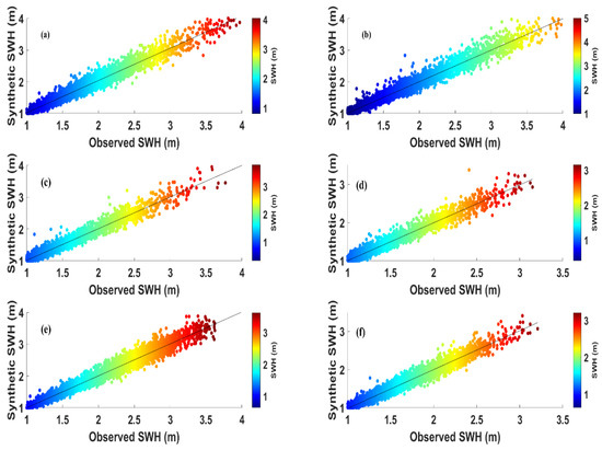
Figure 3.
Scatterplots of synthetic LSTM-generated vs. NDBC-observed significant wave heights (m) for buoys (a) 42056, (b) 42057, (c) 42058, (d) 42059, (e) 41046, and (f) 41047.

Table 3.
Error statistics between LSTM-generated and NDBC observed significant wave height.
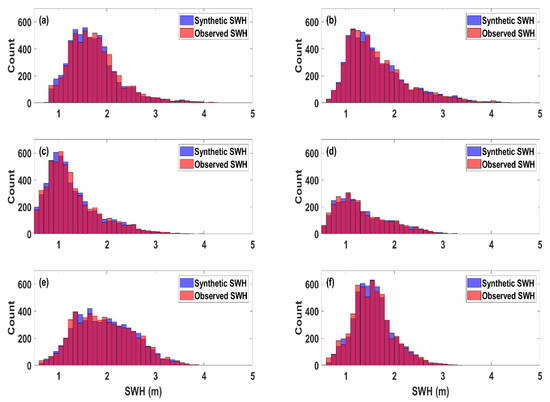
Figure 4.
Histograms of synthetic LSTM-generated vs. NDBC-observed significant wave height (m) for buoys (a) 42056, (b) 42057, (c) 42058, (d) 42059, (e) 41046, and (f) 41047.
3.2. Inverse Modeling
In this subsection, the inversion of wind information from wave properties is performed using the predicted time series. In Figure 5 and Figure 6, scatterplots and histograms of synthetic WSP compared with NDBC observations are presented, with the respective error statistics given in Table 4. Nearly identical to the previous section, it can be observed that LSTM was also highly efficient at converting observed SWH to the corresponding WSP that forced those waves. Specifically, an r2 of 0.99, an RMSE of 0.39 m/s, and a MAPE of 0.07 was returned for buoy 42056 (Figure 5a), an r2 of 0.98, an RMSE of 0.46 m/s, and a MAPE of 0.07 for buoy 42057 (Figure 5b), an r2 of 0.98, an RMSE of 0.46 m/s, and a MAPE of 0.09 for buoy 42058 (Figure 5c), an r2 of 0.98, and an RMSE of 0.26 m/s, and a MAPE of 1.22 for buoy 42059 (Figure 5d). Similar trends were found for buoy 41043 that had an r2 of 0.96, an RMSE of 0.48 m/s, and a MAPE of 0.13 (Figure 5e), and buoy 41046 that had virtually identical r2, RMSE, and MAPE values that were measured at 0.97, 0.48 m/s, and 0.14, respectively (Figure 5f). In Figure 6a–f where in sequence, the scatterplots of NDBC buoys 42056, 42057, 42058, 41043, and 41043 were converted to histograms for a second round of validations, it can be observed that in each case LSTM predictions remain highly accurate when compared with the observations. From MAPE values, however, the inverse modeling of WSP from SWH has greater errors than the conventional modeling of the previous section. This can be explained in that while waves are primarily driven by wind forcing, wind by contrast, in addition to interaction with surface waves [41,42], is affected by a range of other variables not presently considered by LSTM, thus leading to larger errors.
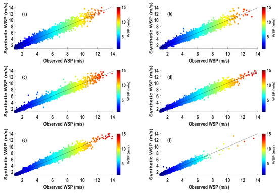
Figure 5.
Scatterplots of LSTM-generated and NDBC-observed significant wave heights (m) for buoys (a) 42056, (b) 42057, (c) 42058, (d) 42059, (e) 41046, and (f) 41047.
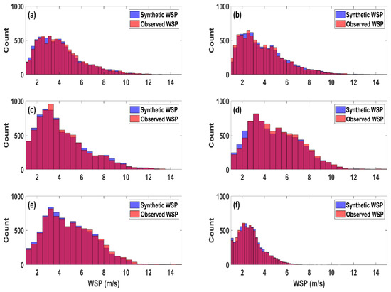
Figure 6.
Histograms of LSTM-generated and NDBC-observed wind speed (m/s) or buoys (a) 42056, (b) 42057, (c) 42058, (d) 42059, (e) 41046, and (f) 41047.

Table 4.
Error statistics between LSTM-generated synthetic surface wind speeds and NDBC observations.
3.3. Applications: Wind and Wave Reconstructions
To further demonstrate the applicability using the LSTM network to simulate variables of interest from available ones, and considering the possibility of complete instrumentation failure, SWAN was used to simulate SWH at NDBC buoys 42058 and 42059 (Figure 1) for September and October 2016 to capture the mean and extreme wave states before, during, and after the passage of Hurricane Matthew (2016). The other buoys were not used given that they were deployed in locations too far from Matthew’s track and thus only recorded mean wind and wave states. Hurricane Matthew (2016) passed through the central Caribbean Sea from 29 September to 3 October (Figure 1) and, at the time, was categorized as a major hurricane with a minimum air pressure of 937 hPa and wind speeds approaching 67 m/s. This is especially relevant given that NDBC buoys 42058 and 42059 have, by 6 June 2020 and 18 October 2020, respectively, gone adrift from their original locations. Data transmissions have halted. In the event of the complete absence of buoys, or their data is of insufficient quality to meet demands, numerical models (once thoroughly validated through other means) are often employed to circumvent these issues and conduct coastal and oceanographic studies [3,43,44]. Demonstrating, we first validate wave simulations using buoy observations in Figure 7. In Figure 7a, r2 and RMSE between the SWH and observations were measured at 0.93 and 1.09, respectively, for NDBC buoy 42058. Similar, albeit poorer, results are shown in Figure 7b for NDBC buoy 42059, where r2 and RMSE were measured at 0.87 and 0.41, respectively. In either figure, although the model was able to reproduce the large-scale features of the measured SWH, fine-scale features were completely missed, leading to the large RMSE values. It is worth noting that through the coupling of an atmospheric model, hurricane-induced SWH could be more realistically simulated due to a better estimation of sea surface roughness [45,46]. This option, however, requires significant computational resources and expertise to set up, couple, and evaluate model results. A significantly cheaper method to increasing SWAN model accuracy was given by Fan et al. that coupled LSTM to the model and increased accuracy by 65% [24]. Following the validation of the simulated SWH, we experiment with reconstructing WSP from these simulations, rather than buoy data (i.e., observations of SWH were completely removed), with results presented in Figure 8.
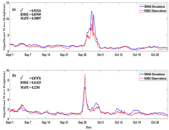
Figure 7.
Validation of SWAN-simulated (blue) and NDBC-observed (red) significant wave height for NDBC buoy 42058 (a) and 42059 (b) before, during, and after the passage of Hurricane Matthew (2016).
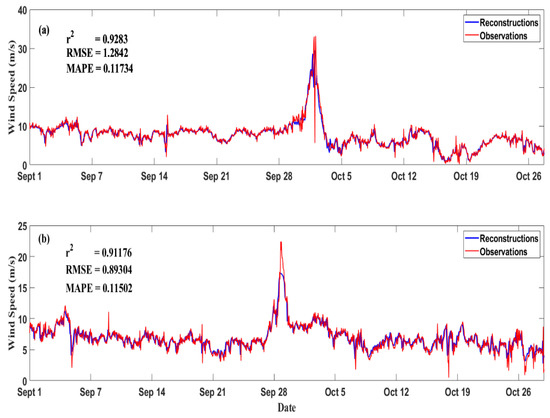
Figure 8.
Comparison of reconstructed (blue) and observed (red) surface wind speed (m/s) at NDBC buoy 42058 (a) and 42059 (b) before, during, and after the passage of Hurricane Matthew (2016).
Observing Figure 8, the inverse modeling of surface wind speed from model-simulated wave heights was highly efficient, reaching an r2, RMSE and MAPE of ~0.93, ~1.3 m/s, and 0.11, respectively, for NDBC buoy 42058 (Figure 8a), and an r2, RMSE, and MAPE of 0.91, 0.89 m/s, and 0.11, respectively, for NDBC buoy 42059 (Figure 8b). However, several high-frequency events were completely missed in each case. Extreme peaks were identically not captured. These results can be strongly contrasted with the wind speed reconstructions of the previous section, where when wave observations were used for inversions, r2 was much higher, and RMSE and MAPE were much lower than where model simulations were used. This result was inevitable due to the accumulation of errors both incurred from usage of the LSTM network and wave model inaccuracies. Thus, while the joint SWAN–LSTM model can help to overcome the lack of robust data due to faulty or absent observation platforms and sensors, extra attention should be placed on ensuring the robustness of SWAN itself to minimize the accumulation of errors.
Additionally, although SWH data are only extracted from the model at two locations, other locations can be selected, and virtual buoys established to perform additional wave studies [47,48,49,50]. At these new locations, using the currently validated SWAN-LSTM model, high fidelity inversions of SWH to WSP can be performed to increase the coverage of ‘observations’ for wind research in general [51,52,53], but co-located wind and wave energy assessments in particular [54,55].
4. Conclusions
For a wide range of coastal and oceanic applications, observations of basic metocean variables are of paramount value, and it is for this reason that wealthy nations have deployed them in large numbers. For small island developing states with neither the financial resources nor expertise to develop, deploy, and maintain these platforms, the data observed by buoys operated by international organizations is even more precious. Thus, methods to fully utilize and, where necessary, reconstruct observations are crucial. This study used a long short-term memory (LSTM) network to initiate the conventional (wind-to-wave) and inverse (wave-to-wind) modeling of observations from six National Buoy Data Center buoys located throughout the Caribbean Sea. In either case, LSTM was highly effective at reproducing winds and waves from their respective counterpart and is thus an extremely attractive option to minimize intermittency on the already sparse buoys regionally deployed in the event of partial instrument failure. Considering the possibility of complete instrument failure, a third-generation numerical wave model was used to produce synthetic wave information before inverse modeling was performed to derive the corresponding surface winds during mean and extreme metocean states. Though ultimately reliant on prior validation through observations and are computationally expensive to use, numerical models offer a significant avenue to simulate wave states with a proven record of efficacy. When coupled with LSTM, the SWAN-LSTM model was able to reconstruct the overlying wind field to a high degree of accuracy. Additionally, the usage of another numerical model to simulate wind speed was completely avoided. It must, however, be repeated that the accuracy of surface wind speed inverted from numerically simulated wave heights is inexorably restricted by the accuracy of the wave model itself. Although this work considered the reconstruction of 1D time-series data, the study can be extended to 2D with the introduction of a convolutional LSTM, and even 3D, with the stacked LSTM.
Author Contributions
Conceptualization, B.J.B. and S.Z.; methodology, B.J.B. and S.Z.; software, B.J.B., S.Z., Y.C., B.J.B. and S.Z.; formal analysis, B.J.B.; investigation, B.J.B., S.Z. and Y.C.; data curation, B.J.B.; writing—original draft preparation, B.J.B.; writing—review and editing, B.J.B. and S.Z.; visualization, B.J.B.; supervision, C.D.; funding acquisition, C.D. All authors have read and agreed to the published version of the manuscript.
Funding
This work was supported by the Southern Marine Science and Engineering Guangdong Laboratory (Zhuhai) (SML2020SP007), the National College Students’ Platform for Innovation and Entrepreneurship Training Program (202010300017Z), and the National Key Research and Development Program of China (2017YFA0604100, 2016YFC1402004 and 2017YFC1404200).
Institutional Review Board Statement
Not Applicable.
Informed Consent Statement
Not Applicable.
Data Availability Statement
Buoy datasets can be acquired at the National Oceanic and Atmospheric Administration’s National Data Buoy Center, available online (https://www.ndbc.noaa.gov/, 25 March 2021).
Acknowledgments
The authors thank the National Oceanic and Atmospheric Administration’s National Data Buoy Center for providing the buoy data used in this paper. Special thanks are extended by B.J.B. to K.T.C. Lim Kam Sian for his help in reviewing and editing an early version of this manuscript and for helpful discussions.
Conflicts of Interest
The authors declare no conflict of interest.
References
- Zhang, B.; Li, X.; Pierre, W.; He, Y. Synergistic measurements of ocean winds and waves from SAR. J. Geophys. Res. Ocean. 2015, 120, 6164–6184. [Google Scholar] [CrossRef]
- Stopa, J.E.; Mouche, A. Significant wave heights from Sentinel-1 SAR: Validation and applications. J. Geophys. Res. Ocean. 2016, 122, 1827–1848. [Google Scholar] [CrossRef]
- Ardhuin, F.; Stopa, J.E.; Chapron, B.; Collard, F.; Husson, R.; Jensen, R.E.; Johannessen, J.; Mouche, A.; Passaro, M.; Quartly, G.D.; et al. Observing Sea States. Front. Mar. Sci. 2019, 6, 124. [Google Scholar] [CrossRef]
- Ribal, A.; Young, I.R. 33 years of globally calibrated wave height and wind speed data based on altimeter observations. Sci. Data 2019, 6, 77. [Google Scholar] [CrossRef]
- Wang, J.; Aouf, L.; Wang, X.; Li, B.; Wang, J. Remote Cross-Calibration of Wave Buoys Based on Significant Wave Height Observations of Altimeters in the Northern Hemisphere. Remote Sens. 2020, 12, 3447. [Google Scholar] [CrossRef]
- Szmytkiewicz, M.; Szmytkiewicz, P.; Marcinkowski, T. Comparison of Design Wave Heights Determined on the Basis of Long- and Short-term Measurement Data. Arch. Hydro-Eng. Environ. Mech. 2018, 65, 123–142. [Google Scholar] [CrossRef]
- Ozkan, C.; Mayo, T. The renewable wave energy resource in coastal regions of the Florida peninsula. Renew. Energy 2019, 139, 530–537. [Google Scholar] [CrossRef]
- Reale, F.; Dentale, F.; Furcolo, P.; di Leo, A.; Carratelli, E.P. An Experimental Assessment of Extreme Wave Evaluation by Integrating Model and Wave Buoy Data. Water 2020, 12, 1201. [Google Scholar] [CrossRef]
- Li, M.; Liu, K. Probabilistic Prediction of Significant Wave Height Using Dynamic Bayesian Network and Information Flow. Water 2020, 12, 2075. [Google Scholar] [CrossRef]
- Matthew, T.E.; Deo, M.C. Inverse estimation of wind from the waves measured by high-frequency radar. Int. J. Remote Sens. 2010, 33, 2985–3003. [Google Scholar] [CrossRef]
- Kirinchich, A. Remote Sensing of the Surface Wind Field over the Coastal Ocean via Direct Calibration of HF Radar Backscatter Power. J. Atmos. Ocean. Technol. 2015, 33, 1377–1392. [Google Scholar] [CrossRef]
- Shen, W.; Gurgel, K. Wind Direction Inversion from Narrow-Beam HF Radar Backscatter Signals in Low and High Wind Conditions at Different Radar Frequencies. Remote Sens. 2018, 10, 1480. [Google Scholar] [CrossRef]
- Fujimura, A.; Lehner, S.; Soloviev, A.; Li, X. Sea surface roughness observed by high resolution radar. Remote Sens. 2019, 11, 2026. [Google Scholar] [CrossRef]
- Pan, H.; Gao, P.; Zhou, H.; Ma, R.; Yang, J.; Zhang, X. Roughness Analysis of Sea Surface from Visible Images by Texture. IEEE Access 2020, 8, 46448–46458. [Google Scholar] [CrossRef]
- Daga, M.; Deo, M.C. Alternative data-driven methods to estimate wind from waves by inverse modeling. Natural Hazards. J. Int. Soc. Prev. Mitig. Nat. Hazards 2009, 49, 293–310. [Google Scholar]
- Kambekar, A.R.; Deo, M.C. Wave simulation and forecasting using wind time history and data-driven methods. Ships Offshore Struct. 2010, 5, 253–266. [Google Scholar] [CrossRef]
- Nitsure, S.P.; Londhe, S.N.; Khare, K.C. Wave forecasts using wind information and genetic programming. Ocean. Eng. 2012, 54, 61–69. [Google Scholar] [CrossRef]
- Charhate, S.B.; Deo, M.C.; Londhe, S.N. Inverse modeling to derive wind parameters from wave measurements. Appl. Ocean. Res. 2008, 30, 120–129. [Google Scholar] [CrossRef]
- Akbarifard, S.; Radmanesh, F. Predicting sea wave height using Symbiotic Organisms Search (SOS) algorithm. Ocean. Eng. 2018, 167, 348–356. [Google Scholar] [CrossRef]
- James, S.C.; Zhang, Y.; O’Donncha, F. A machine learning framework to forecast wave conditions. Coast. Eng. 2018, 137, 1–10. [Google Scholar] [CrossRef]
- Vieira, F.; Cavalcante, G.; Campos, E.; Taveira-Pinto, F. A methodology for data gap filling in wave records using Artificial Neural Networks. Ocean. Eng. 2020, 98, 102109. [Google Scholar] [CrossRef]
- Ni, C.; Ma, X. An integrated long-short term memory algorithm for predicting polar westerlies wave height. Ocean. Eng. 2020, 215, 107715. [Google Scholar] [CrossRef]
- Pushpam, M.M.P.; Enigo, F.V.S. Forecasting Significant Wave Height using RNN-LSTM Models. In Proceedings of the 4th International Conference on Intelligent Computing and Control Systems (ICICCS), Madurai, India, 13–15 May 2020; pp. 1141–1146. [Google Scholar] [CrossRef]
- Fan, S.; Xiao, N.; Dong, S. A novel model to predict significant wave height based on long short-term memory network. Ocean. Eng. 2020, 205, 107298. [Google Scholar] [CrossRef]
- Booij, N.; Ris, R.C.; Holthuijsen, L.H. A third-generation wave model for coastal regions: 1. Model description and validation. J. Geophys. Res. Ocean. 1999, 104, 7649–7666. [Google Scholar] [CrossRef]
- Booij, N.; Holthuijsen, L.; Battjes, J. Ocean to near-shore wave modelling with SWAN. Conf. Coast. Dyn. 2001, 335–344. [Google Scholar] [CrossRef]
- Phillips, O.M. On the generation of waves by turbulent wind. J. Fluid Mech. 1957, 2, 417–445. [Google Scholar] [CrossRef]
- Miles, J.W. On the generation of surface waves by shear flows. J. Fluid Mech. 1960, 3, 185–204. [Google Scholar] [CrossRef]
- Hasselmann, K. On the spectral dissipation of ocean waves due to white capping. Bound. Layer Meteorol. 1974, 6, 107–127. [Google Scholar] [CrossRef]
- The Wamdi Group. The WAM model—A third generation ocean wave prediction model. J. Phys. Oceanogr. 1988, 18, 1775–1810. [Google Scholar] [CrossRef]
- Hasselmann, K. Measurements of wind-wave growth and swell decay during the joint North Sea wave project (JONSWAP). Dtsch. Hydrogr. Z. 1973, 12, 1–95. [Google Scholar]
- Collins, J.I. Prediction of shallow-water spectra. J. Geophys. Res. 1972, 77, 2693–2707. [Google Scholar] [CrossRef]
- Madsen, O.S.; Poon, Y.K.; Graber, H. Spectral wave attenuation by bottom friction: Theory. In Proceedings of the Twenty-First International Conference on Coastal Engineering. American Society of Civil Engineers, Torremolinos, Spain, 20–25 June 1988; pp. 492–504. [Google Scholar]
- Battjes, J.A.; Janssen, J.P.F.M. Energy loss and set-up due to breaking of random waves. Coast. Eng. 1978, 569–587. [Google Scholar] [CrossRef]
- Hasselmann, S.; Hasselmann, K.; Allender, J.H.; Barnett, T.P. Computations and parameterizations of the nonlinear energy transfer in a gravity wave spectrum. Part II: Parameterizations of the nonlinear transfer for application in wave models. J. Phys. Oceanogr. 1985, 15, 1378–1391. [Google Scholar] [CrossRef]
- Holthuijsen, L.H.; Herman, A.; Booij, N. Phase-decoupled refraction–diffraction for spectral wave models. Coast. Eng. 2003, 49, 291–305. [Google Scholar] [CrossRef]
- Cavaleri, L.; Rizzoli, P.M. Wind wave prediction in shallow water: Theory and applications. J. Phys. Oceanogr. 1981, 86, 10961–10973. [Google Scholar] [CrossRef]
- Tolman, H.L. User Manual and System Documentation of WAVEWATCH III TM Version 3.14; NOAA/NWS/NCEP/MMAB Technical note 276; U.S. Department of Commerce, National Oceanic and Atmospheric Administration National Weather Service, National Centers for Environmental Prediction: College Park, MD, USA, 2009; p. 187.
- Choi, J.Y.; Lee, B. Combining LSTM Network Ensemble via Adaptive Weighting for Improved Time Series Forecasting. Math. Probl. Eng. 2018, 2018, 2470171. [Google Scholar] [CrossRef]
- Yu, Y.; Si, X.; Hu, C.; Zhang, J. A Review of Recurrent Neural Networks: LSTM Cells and Network Architectures. Neural Comput. 2019, 31, 1235–1270. [Google Scholar] [CrossRef]
- Babanin, A.V.; McConochie, J.; Chalikov, D. Winds near the surface of waves: Observations and Modeling. J. Phys. Oceanogr. 2018, 48, 1079–1088. [Google Scholar] [CrossRef]
- Chen, S.; Qiao, F.; Jiang, W.; Guo, J.; Dai, D. Impact of Surface Waves on Wind Stress under Low to Moderate Wind Conditions. J. Phys. Oceanogr. 2019, 49, 2017–2028. [Google Scholar] [CrossRef]
- Walker, J.; Murphy, E.; Ciardulli, F.; Hamm, L. On the Reliance on Modelled Wave Data in the Arabian Gulf for Coastal and Port Engineering Design. Coast. Eng. Proc. 2014, 1, 28. [Google Scholar] [CrossRef]
- Jiang, H. Indirect Validation of Ocean Remote Sensing Data via Numerical Model: An Example of Wave Heights from Altimeter. Remote Sens. 2020, 12, 2627. [Google Scholar] [CrossRef]
- Lim Kam Sian, K.T.C.; Dong, C.; Lu, H.; Wu, R.; Zhang, H. Effects of Model Coupling on Typhoon Kalmaegi (2014) Simulation in the South China Sea. Atmosphere 2020, 11, 432. [Google Scholar] [CrossRef]
- Kumar, R.; Sandeepan, B.S.; Holland, D.M. Impact of different sea surface roughness on surface gravity waves using a coupled atmosphere-wave model: A case of Hurricane Isaac (2012). Ocean. Dyn. 2020, 70, 1–13. [Google Scholar]
- Ponce de Leon, S.; Orfila, A.; Simarro, G. Wave energy in the Balearic Sea. Evolution from a 29 year spectral wave hindcast. Renew. Energy 2016, 85, 1192–1200. [Google Scholar] [CrossRef]
- Dentale, F.; Furcolo, P.; Carratelli, E.P.; Reale, F.; Contestabile, P.; Tomasicchio, G.R. Extreme Wave Analysis by Integrating Model and Wave Buoy Data. Water 2018, 10, 373. [Google Scholar] [CrossRef]
- Jury, M. Characteristics and Meteorology of Atlantic Swells Reaching the Caribbean. J. Coast. Res. 2018, 34, 400–412. [Google Scholar] [CrossRef]
- Vega, M.J.; Alvarez-Silva, O.; Restrepo, J.C.; Ortiz, J.C.; Otero, L.J. Interannual variability of wave climate in the Caribbean Sea. Ocean. Dyn. 2020, 70. [Google Scholar] [CrossRef]
- Wentz, F.J. Evaluating and extending the ocean wind climate data record. IEEE J. Sel. Top. Appl. Earth Obs. Remote Sens. 2017, 10, 2165–2185. [Google Scholar] [CrossRef]
- Dukhovskoy, D.S.; Bourassa, M.A.; Petersen, G.N.; Steffen, J. Comparison of the ocean surface vector winds from atmospheric reanalysis and scatterometer-based wind products over the Nordic Seas and the northern North Atlantic and their application for ocean modeling. J. Geophys. Res. Ocean. 2017, 122, 1943–1973. [Google Scholar] [CrossRef]
- Golbazi, M.; Archer, C.L. Methods to Estimate Surface Roughness Length for Offshore Wind Energy. Adv. Meteorol. 2019, 2019, 5695481. [Google Scholar] [CrossRef]
- Pérez-Collazo, C.; Jakobsen, M.M.; Buckland, H.; Fernández-Chozas, J. Synergies for a Wave-Wind Energy Concept; EWEA: Frankfurt, Germany, 2013. [Google Scholar]
- Azzellino, A.; Lanfredi, C.; Riefolo, L.; de Santis, V.; Contestabile, P.; Vicinanza, D. Combined Exploitation of Offshore Wind and Wave Energy in the Italian Seas: A Spatial Planning Approach. Front. Energy Res. 2019, 7, 42. [Google Scholar] [CrossRef]
Publisher’s Note: MDPI stays neutral with regard to jurisdictional claims in published maps and institutional affiliations. |
© 2021 by the authors. Licensee MDPI, Basel, Switzerland. This article is an open access article distributed under the terms and conditions of the Creative Commons Attribution (CC BY) license (https://creativecommons.org/licenses/by/4.0/).