Article

Flow Field Measurement of Laboratory-Scaled Cross-Flow Hydrokinetic Turbines: Part I—The Near-Wake of a Single Turbine

Department of Mechanical Engineering, Keio University, Yokohama 223-8522, Japan
*
Author to whom correspondence should be addressed.
J. Mar. Sci. Eng. 2021, 9(5), 489; https://doi.org/10.3390/jmse9050489
Submission received: 7 April 2021 / Revised: 26 April 2021 / Accepted: 27 April 2021 / Published: 1 May 2021
(This article belongs to the Section Ocean Engineering)

Abstract

:
Recent developments in marine hydrokinetic (MHK) technology have put the cross-flow (often vertical-axis) turbines at the forefront. MHK devices offer alternative solutions for clean marine energy generation as a replacement for traditional hydraulic turbines such as the Francis, Kaplan, and Pelton. Following previous power measurements of laboratory-scaled cross-flow hydrokinetic turbines in different configurations, this article presents studies of the water flow field immediately behind the turbines. Two independent turbines, which operated at an average diameter-based Reynolds number of approximately 0.2 × 10 5 , were driven by a stepper motor at various speeds in a closed circuit water tunnel with a constant freestream velocity of 0.316 m/s. The wakes produced by the three NACA0012 blades of each turbine were recorded with a monoscopic particle image velocimetry technique and analyzed. The flow structures with velocity, vorticity, and kinetic energy fields were correlated with the turbine power production and are discussed herein. Each flow field was decomposed into the time averaged, periodic, and random components for all the cases. The results indicate the key to refining the existed turbine design for enhancement of its power production and serve as a baseline for future comparison with twin turbines in counter-rotating configurations.

1. Introduction

In early 2021, while countries around the world were starting to ease their measures against the COVID-19 pandemic and slowly implementing economic recovery policies, records of renewable energy projects were broken. During 2021–2024, the highest amount ever of approximately 50 GW of new renewable capacity awarded by 13 countries will become operational [1]. On the global scale, the hydropower sector is expected to grow to USD 1510 billion in 2025 and currently occupies about 60% of the renewable energy market [2]. Although the traditional method of hydropower extraction is considered clean and renewable, its required constructions of hydraulic dams often create negative impacts on the neighboring environment and society. Lessons should be learned from giant hydropower plants such as the Three Gorges project that has affected and dislocated millions of people [3,4,5]. One of the established directions to design and develop low-head hydro devices, supported by the US National Renewable Energy Laboratory (NREL), mimics commercial lift-based wind turbines and results in marine hydrokinetic (MHK) turbines that do not require any hydraulic dams. Similar to well-developed wind turbines, MHK devices, which can generate electricity from different water resources such as ocean currents, tides, and rivers, are often categorized into axial-flow and cross-flow design.
Recent efforts in MHK technology development have sparked interest in pair configurations of cross-flow (vertical-axis) turbines due to their ability to enhance system energy output over a unit area. In the wind energy literature, co-rotating and counter-rotating configurations of vertical-axis wind turbines (VAWTs) were pioneered by John Dabiri back in 2011 [6]. In 2019, Brownstein et al. (Dabiri Group) recorded a 14% enhancement of array performance of pair configurations of VAWTs in a wind tunnel setup at the diameter-based Reynolds number (Re) of 0.73 × 10 5 [7]. Additionally, Jiang et al. also experimentally observed a 38.6% enhancement of array power output with a deflector between a pair of VAWTs [8]. In the MHK literature, a twin system of MHK turbines was first experimentally examined by Li and Calisal in a tow tank facility [9,10]. Due to their potential of increasing the system power output per unit of occupied area, cross-flow MHK turbines remain a strong experimental as well as numerical topic of research, which usually focuses on turbine design for optimal power production, hydrodynamic interaction between devices in arrays, and environmental effects such as surface wave and channel blockage on device power output [11,12,13,14,15,16,17,18,19].
While numerical works are popular in the MHK literature, the number of published experimental studies has been limited due to difficulties in implementation of mechanical systems and electronics underwater. Instantaneous flow field measurements are usually not possible for scalable experiments in a tow tank facility. On the other hand, small-scaled experiments in a water tunnel, though not scalable, can suggest trends and directions for bigger engineering systems. Although instantaneous flow field measurements have been done for those laboratory-scaled cross-flow turbine experiments [20], most of the time, related turbine power measurement cannot be done for such a small scale.
Operating at the diameter-based Reynolds number of 0.2 × 10 5 , the laboratory-scaled experiment of cross-flow MHK turbines discussed in this article was first observed to exhibit power enhancement in some specific counter-rotating configurations in 2018 [21]. Attempts of relevant computational fluid dynamic (CFD) models faced difficulties in model validation and convergence [22,23]. By extending the work of Markovic in system mechanical loss measurement [24] and improving the experimental method in [21], a novel method was implemented and applied to the turbine system, which resulted in more reliable and accurate measurement of the system power output in different configurations [25]. The natural extension of this work is to capture the relevant flow field around the turbines and observe any correlation with the power output.
In this article, the near-wake flow fields of the two independent identically manufactured laboratory-scaled cross-flow MHK turbines, shown in [21,22,23,25], are presented and discussed in terms of flow velocity, energy budget, and, for the first time, correlation with turbine power output at various rotational speeds. All experiments presented in this study adopted a time-resolved mono-scopic particle image velocimetry (2D PIV) technique in a small water tunnel facility. The results not only play an important role in further turbine optimization but also lay the first foundation for future CFD model validation as well as a follow-up comparison between a single turbine and devices in counter-rotating configurations. The wake structure behind a turbine system also provide valuable information to optimize multiple devices in a power farm. It is also worth mentioning that experimentally obtaining an MHK turbine wake is an arduous task, so there are only a few relevant studies in the literature [20,26]. The ultimate goal of this series is to optimize a twin turbine system, in terms of power production and hydrodynamics, in counter-rotating configurations through a series of experiments and numerical simulations.

2. Apparatus and Methodology

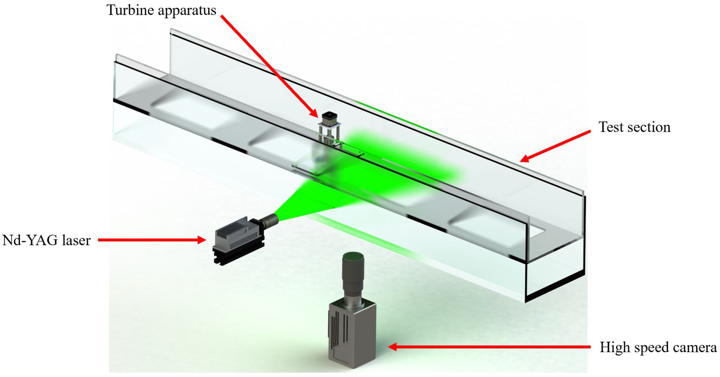
Experiments presented in this paper took place in a laboratory-scaled circulating water tunnel illustrated in Figure 1. While the turbine apparatus and flume facility were already discussed in detail in [25], key components and factors that influenced the flow measurement results are shown in this section for the reader’s convenience. The water tunnel includes a transparent test section 2 m long, 0.27 m wide, and 0.135 m deep. All the experiments were conducted at a fixed inlet velocity U of 0.316 m/s and a turbulence intensity of 4%. The turbine apparatus, shown in Figure 2, was positioned in the middle of the test section at a blockage ratio of β = 19.3 % , which is defined as the ratio of the turbine frontal area over the channel cross-sectional area.

2.1. Turbine Towers and Mechanical Design

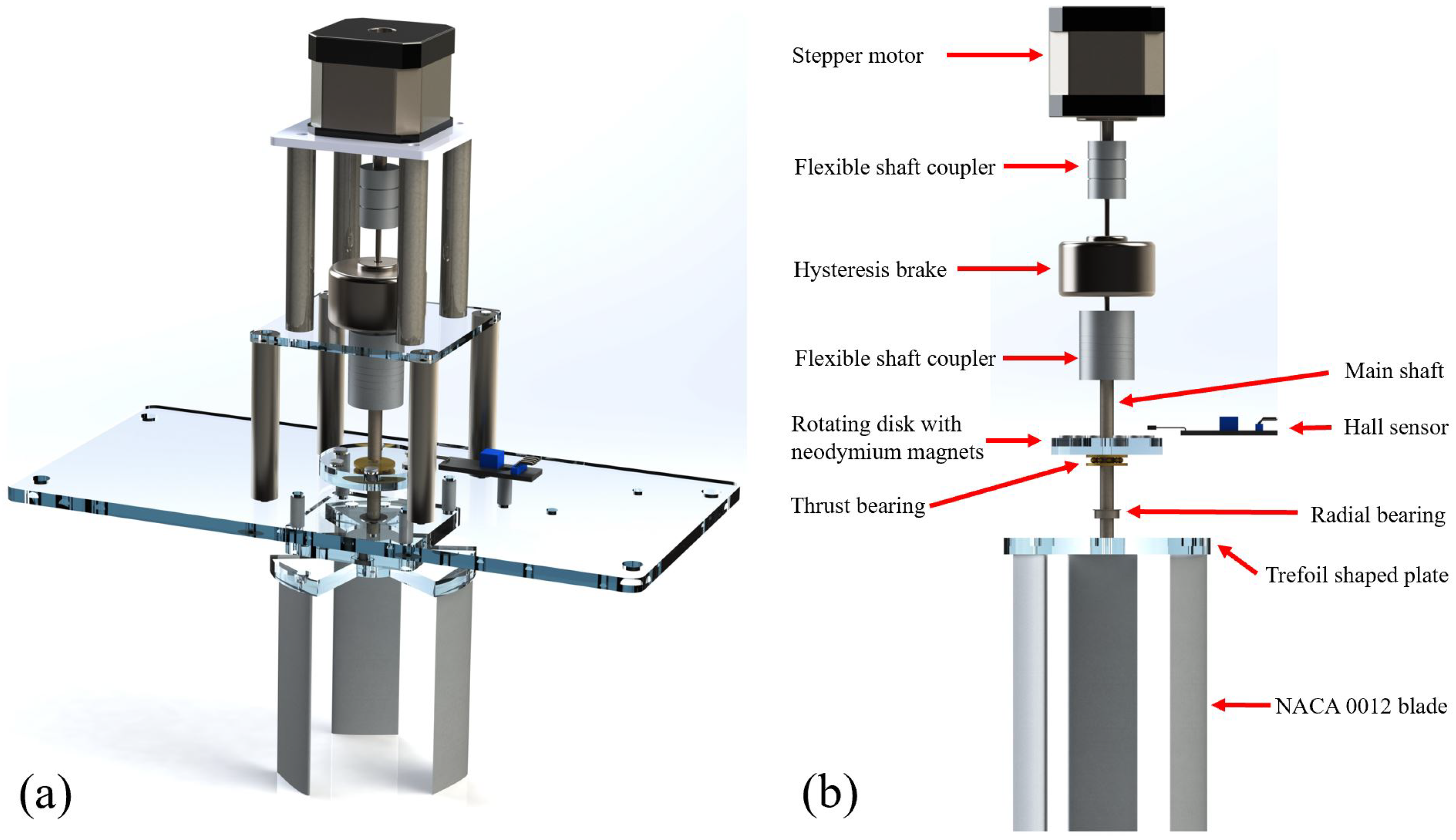
The apparatus overview and its critical components are illustrated in Figure 3. For both illustration and fabrication purposes, Figure 1, Figure 3 and Figure 4 were drawn in SolidWorks based on relevant physical dimensions and rendered by PhotoView 360. The whole turbine is mounted on a 5 mm thick acrylic support plate. This tower was a combination of a Nema 17 stepper motor, a Kimchen HB-300 hysteresis brake, a rotating acrylic disk with six equally spaced neodymium magnets, and a turbine assembly. The turbine shaft was mechanically supported by one radial ball bearing and one thrust roller bearing. All shafts were connected by 2 flexible aluminum couplers. This design allows rapid switching of the turbine assembly, through an M2 bolt, at the bottom of the tower, so that experiments could be conducted with different turbine configurations. All the experiments presented in this article were conducted with 2 single-turbine configurations, which are further explained in the section below.

2.2. Electronics

During a flow measurement session, the turbine was driven at a constant speed, within a 0.05% standard deviation, by the NEMA 17 stepper motor, which was controlled by an L298N driver and an Arduino Mega micro-controller. The speed was simultaneously measured with the magnet/Hall sensor system described in [25]. This Hall sensor detected the magnetic fields of the six rotating neodymium magnets (Figure 2b) as a function of time at 5 KHz. As the magnets are equally spaced and rotate with the turbine, the rotational speed could be calculated as the full angular spacing divided by the time difference between the detection of each magnet. Instead of being water-flow-driven as in the previous power measurement experiments, the turbine rotational speed was motor-controlled at a fixed value to help with the convergence of phase-averaged flow measurement results. Motor-driven experiments could be expected to reproduce the physics of the flow-driven turbines, as proven by Araya and Dabiri [27]. To minimize the amount of modification of the power measurement apparatus, the brake was kept intact, and its voltage supply was kept at zero, so that no additional braking torque was exerted on the turbine shaft. Lastly, water temperature before and after each particle image velocimetry (PIV) experiment was recorded by a type K thermocouple and an A&D AD-5601A digital reader.

2.3. Particle Image Velocimetry

A monoscopic PIV system was set up to capture the planar water flow in the near-wake region of each turbine configuration. The system, shown in Figure 3, contains a Photron FASTCAM SA3 camera and an Nd-YAG laser. The camera, located under the transparent test section, recorded images of the region of interest at 500 frames/s with a 35–200 mm Nikon lens. Polyamide 12 (90 μm diameter) seeding particles were injected into the water flume to visualize the flow behind the turbine configurations. These particles were illuminated by the 2 W 532 nm Nd-YAG laser sheet, which was aligned with the incoming flow and perpendicular to the turbine axis. The laser sheet (PIV measurement plane) location was fixed at 3 cm from the blade tips. Since the blades were submerged approximately 8 cm under-water, the plane location was selected to minimize the out-of-plane motion while avoiding any air pockets drawn into the flow from the water–air interface. The measurement plane was calibrated by a matrix of 29 by 29 white dots (4 mm diameter and 6 mm spacing) on a black background. The uncertainty of this measurement technique was previously estimated to be within 5% in the streamwise direction and 2.5% in the transverse direction of the freestream velocity [22,28,29].
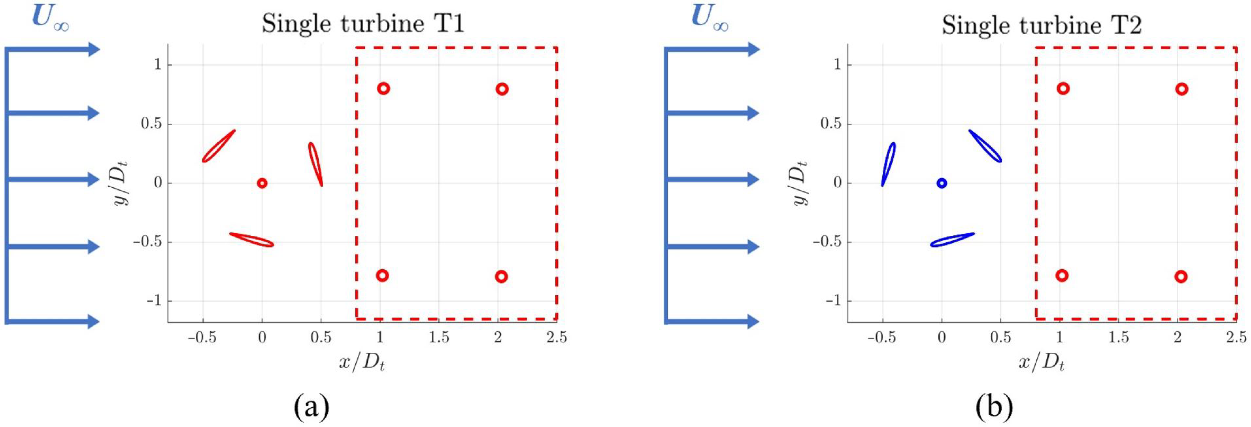
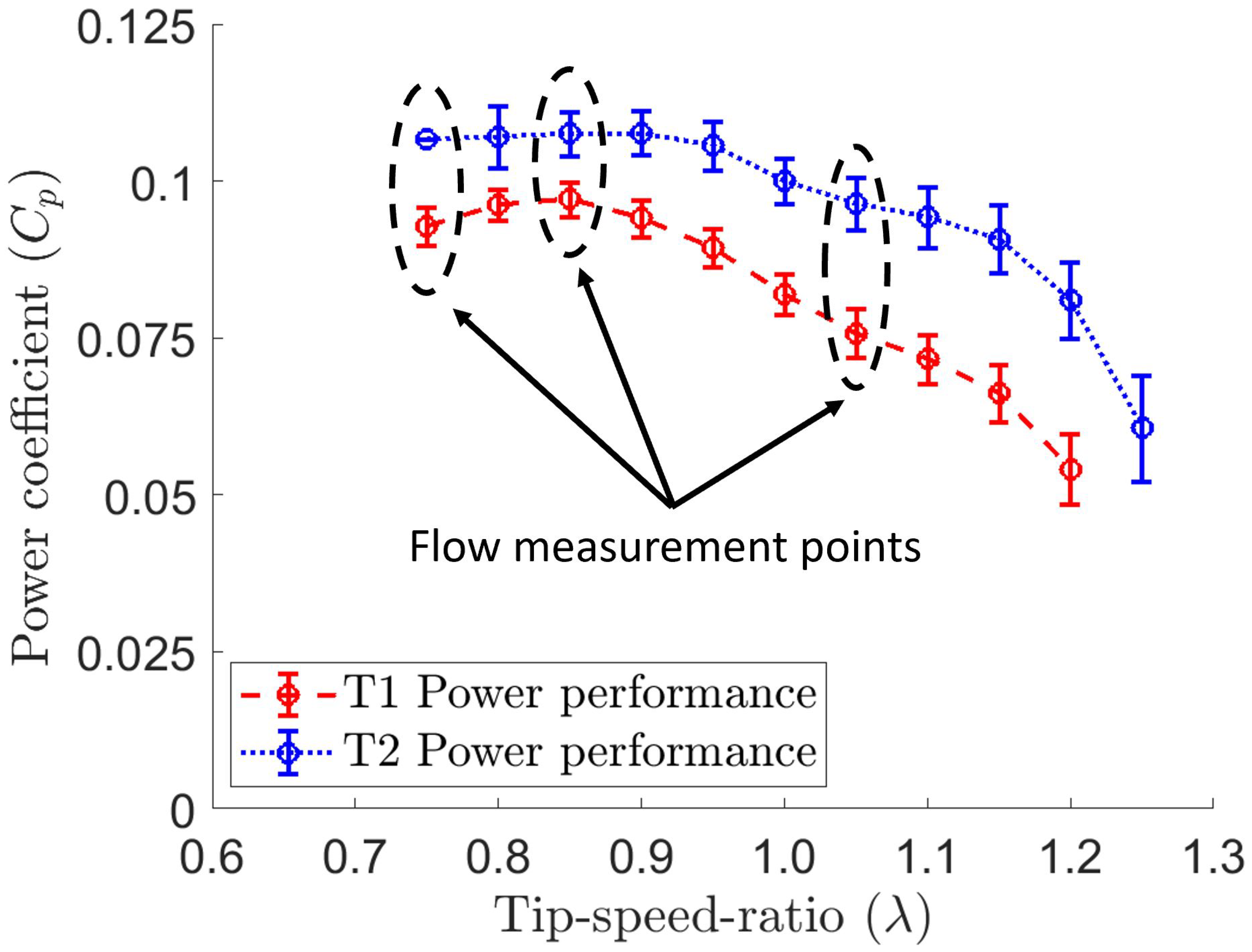
The near-wake regions of the single turbine T1 and T2, discussed in [25], were captured by this PIV setup at various rotational speeds. Each turbine assembly was fabricated by mounting 3 aluminum straight blades on a trefoil-shaped acrylic plate. The 10 cm long blades were electric discharge machined, based on the NACA0012 profile of 25.4 mm chord length, and bolted at a radius of 34.14 mm and a fixed pitch angle of 15 . Additionally, the blades were arranged so that the two assembled turbines T1 and T2 possessed opposite rotational directions. The turbines are theoretically identical and should have exhibited exactly the same power curve. In reality, the power measurement results showed that their power curves are slightly different. Figure 5 shows T1 configuration (a), T2 configuration (b), flow measurement region (enclosed by the red dashed lines), and 4 arbitrary points (red circles) that were selected to extract time-series data for fast Fourier transformation (FFT) and convergence analyses. The experiments were conducted at 3 different turbine speed values, which correspond to the 3 cases of the tip-speed-ratio (1) λ = 0.75 < 1 ; (2) λ = 0.85 , where the power coefficient was measured to attained its maximal value; and (3) λ = 1.05 > 1 . The tip-speed ratio λ is defined as ω R t / U , where ω is the turbine rotational speed and R t is the turbine radius. The previously measured power curves of the turbines and the flow measurement points are displayed in Figure 6 for the readers’ convenience. The PIV calculation area was specified by a matrix of 48 by 62 points spreading from 0.8 to 2.5 in the streamwise direction (x) and −1.15 to 1.15 in the channel wall normal direction (y). These values are non-dimensionalized by the turbine diameter. The channel walls, which are not shown in the figures, are located at approximately x = ± 2.0 . During one continuous data capturing session, the Photron camera memory was able to record 8187 realizations (or more than 16 s at 500 frame/s) of the flow, which resulted in different numbers of turbine rotations depending on the input rotational speed. Therefore, convergence of the near-wake results first needed to be considered for each individual data set.
For each configuration, three data sets were recorded and merged, giving a total of more than 24,000 realizations (or more than 48 s) of the flow. Another pair of magnet and Hall sensor was implemented as a camera trigger so that all 3 data sets were initiated at approximately the same initial phase angle. The extra neodymium magnet was mounted on the trefoil shaped plate so that it rotated with one turbine blade, while the Hall sensor was fixed on the acrylic structural frame. Once the sensor detected the magnet presence, it sent out a digitally high signal. In every data-initiating event, the camera was given an idling signal from the control computer and then waited for the second signal from the Hall sensor to actually start video-recording.
The phase angle Φ , by definition, reaches its zero value when one of the blades is at the position where it encounters the maximum relative velocity of the flow. Turbine T2, for instance, in Figure 5b is at Φ = 0 . The other phases are defined as the angular displacement between the nearest blade and the zero angle. For example, turbine T1 in Figure 5a is at Φ = 60 .

3. Results and Discussion

Fast Fourier transformation analysis was firstly done to determine an appropriate frequency and time period to be used for further convergence studies and phase-averaged analyses of the flow fields.

3.1. Fast Fourier Analysis

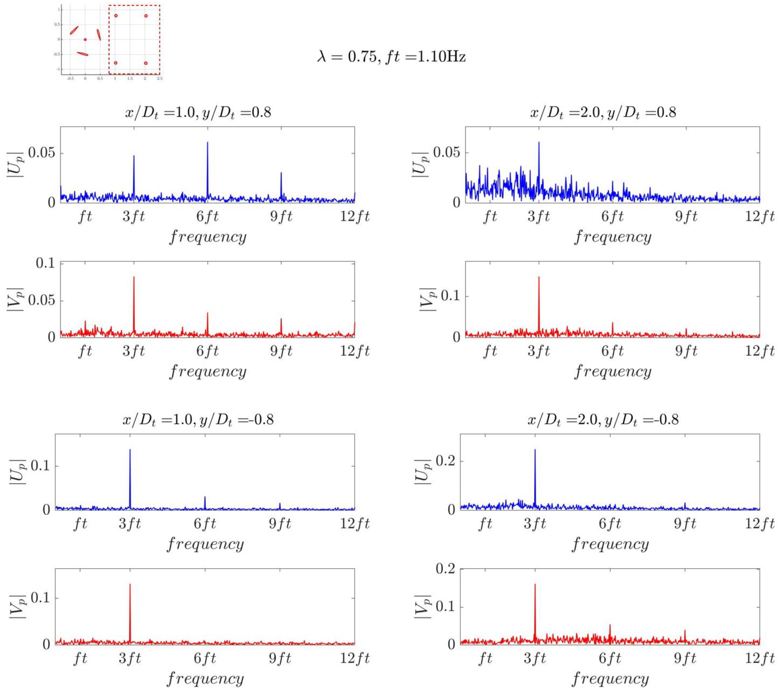
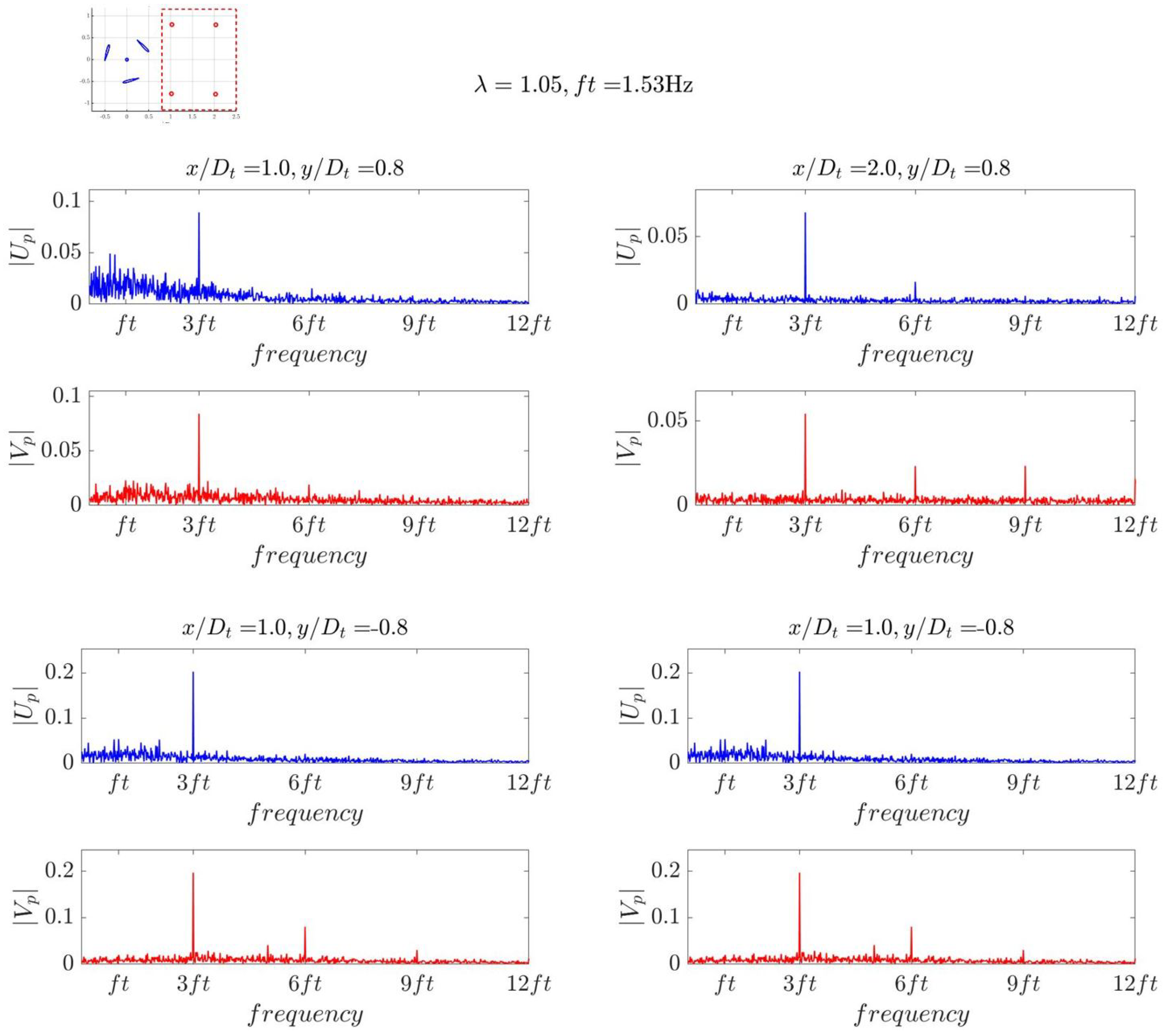
The time-series velocity data at four arbitrary points, shown in Figure 5, in the wake was extracted to perform fast Fourier transformation. The data of each turbine configuration at three different rotational speeds was input into the Matlab discrete Fourier transform function [30] to compute the power amplitudes of the non-dimensionalized streamwise | U p | and transverse | V p | velocity component on the frequency domain. Figure 7 and Figure 8, which show examples of the FFT analyses of the T1 configuration at λ = 0.75 and the T2 configuration at λ = 1.05 , indicate that 3 times the turbine rotating frequency 3 f t is the dominating component of the velocity power spectra. This tendency was observed in all experiments, which is consistent with the fact that each turbine has 3 blades, and therefore one third of the turbine full rotation can be taken as a periodic phase of the flow field.

3.2. Data Convergence

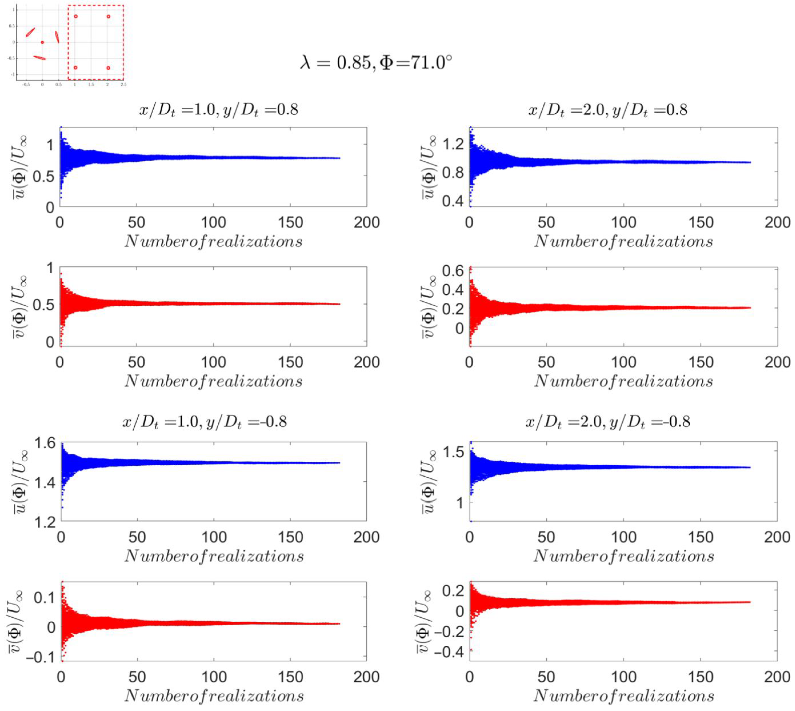
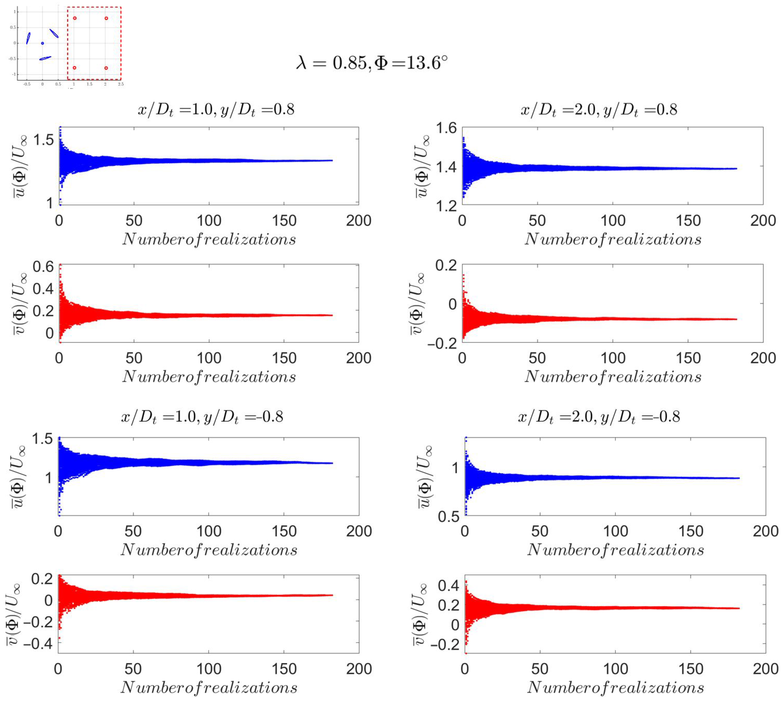
As the FFT analyses suggest that the mean flow has strong periodicity every one-third of a full turbine rotation (one phase), the data convergence study was conducted by computing the mean flow of the four points shown in Figure 5 at a specific phase angle Φ over different numbers of phases. Although the maximum numbers of phases obtained with 24,561 realizations were different depending on the turbine speed, Figure 9 and Figure 10 show the velocity components of the four points being leveled out at more than 100 realizations at a specific phase angle Φ . This behavior was also recorded for all other experiments and phase angles, which indicates statistically converged field data sets. The results presented in the rest of this article were post-processed with the maximum number of phases recorded at the corresponding turbine speed.

3.3. Mean Flow

The recorded 2D instantaneous velocity fields, with the streamwise u and transverse v component, can be decomposed as
u ( Φ , t ) = u ¯ + u ˜ + u ,
v ( Φ , t ) = v ¯ + v ˜ + v ,
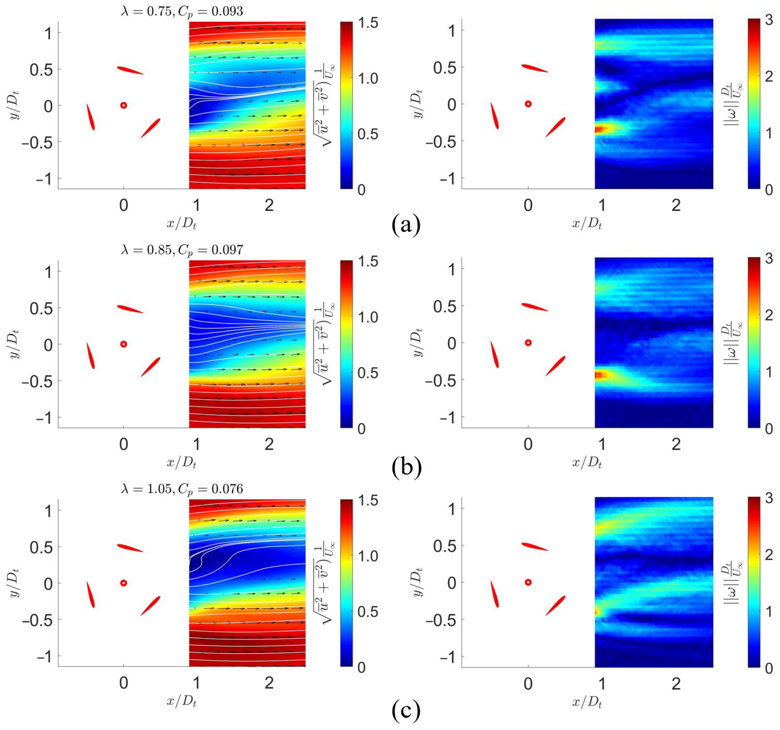
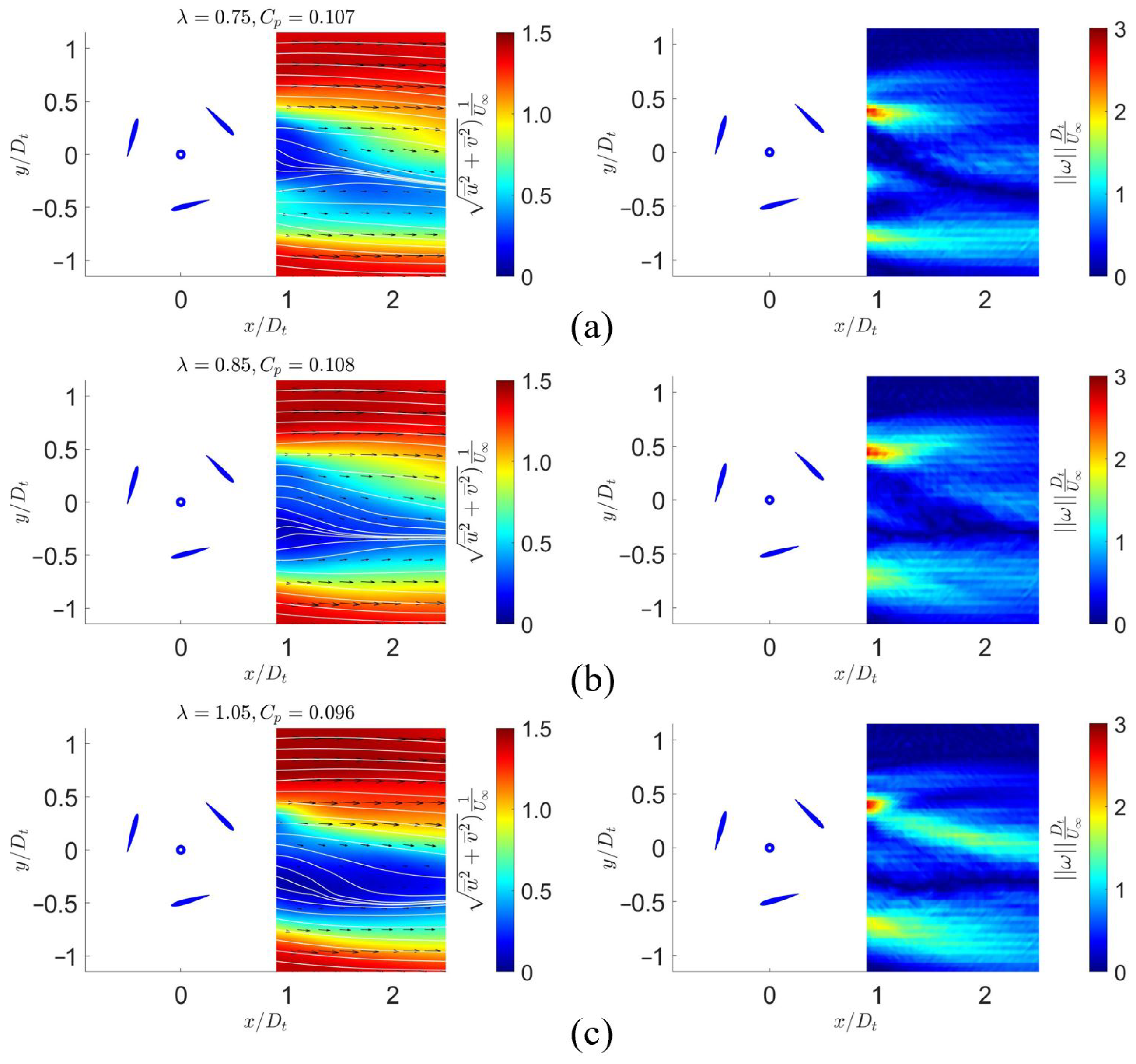
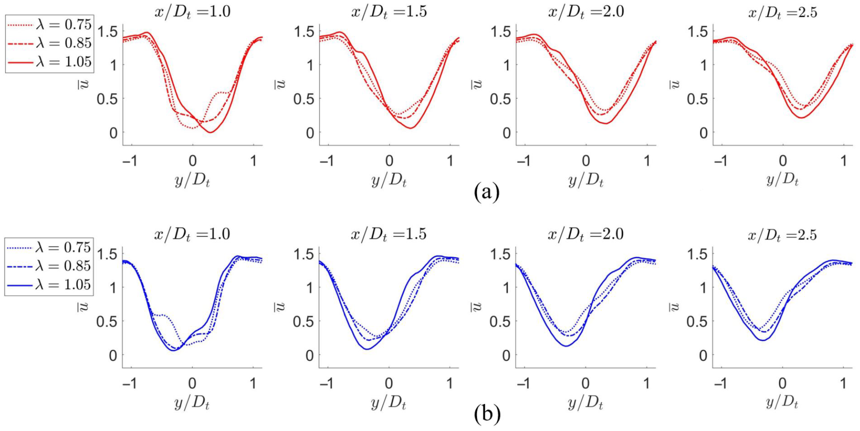
where u ¯ and v ¯ are the time averaged components, u ˜ and v ˜ are periodic components due to different turbine phase angles Φ , and u and v are the random components due to turbulence. This idea of decomposing the flow velocity into three components has been widely adopted by fluid mechanics experimentalists [31,32]. Figure 11 and Figure 12 show the time-averaged flow fields of the two turbines at the three different tip–speed ratios with their corresponding reference power coefficient C P published in [25]. The velocity vector fields and corresponding streamlines are plotted in Figure 11 and Figure 12 with the color maps of the velocity magnitude u ¯ 2 + v ¯ 2 , while Figure 13 displays the streamwise velocity at different locations in the wake. For each individual turbine, the higher the reference power coefficient is, the less skewed the streamlines at that corresponding turbine speed were observed in Figure 11 and Figure 12. The skewness of the streamlines could also be seen in the streamwise velocity plots in Figure 13. The least skewed curves are the cases of λ = 0.85 , which correspond to the maximum measured power production. The skewness of the streamlines in fact represents the amount of body force exerted on the control volume, which is correlated with power losses. Furthermore, the non-dimensionalized vorticity magnitude shown in Figure 11 and Figure 12 indicates a correlation between the turbine power and the amount of vorticity in the wake. Turbines should be designed to reduce the vorticity magnitude in the wake, which represents velocity gradient or losses due to shear stresses in the flow.
Although the two turbines exhibited qualitatively similar near-wake structures, a few minor differences can be observed in Figure 11, Figure 12 and Figure 13. At λ = 0.75 and λ = 1.05 , the streamlines on turbine T1 plots show noticeably swirling motions compared to turbine T2. Additionally, the same swirling structures could be seen in individual phases of turbine T2, which suggests these structures did not appear consistently at the same location. In other words, the three blades of turbine T2 might have been mounted at slightly greater differences in radius and pitch angle, which also explains the difference in the turbine power curves in [25]. The uncertainties in the turbine radius and pitch angle were estimated to be 0.5 mm and 0 . 5 . In terms of energy production, the power extracted by each turbine is the difference between the fluid power going in subtracted by the mechanical loss and the fluid power going out into the wake. With the recorded flow fields in the wake, the fluid kinetic energy behind each turbine, which represents the power loss, was further analyzed.

3.4. Kinetic Energy

Similar to the velocity components, the fluid kinetic K can be decomposed into three components: the mean K ¯ , periodic K ˜ , and random component K , which are defined as
K ¯ = 1 2 ( u ¯ 2 + v ¯ 2 ) ,
K ˜ ( Φ ) = 1 2 ( u ˜ 2 + v ˜ 2 ) ,
K ( Φ ) = 1 2 ( u 2 + v 2 ) ,
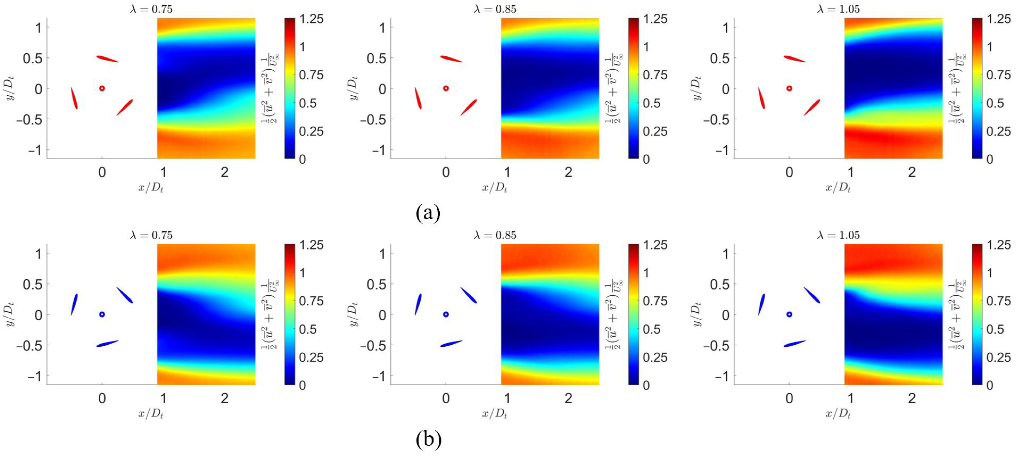
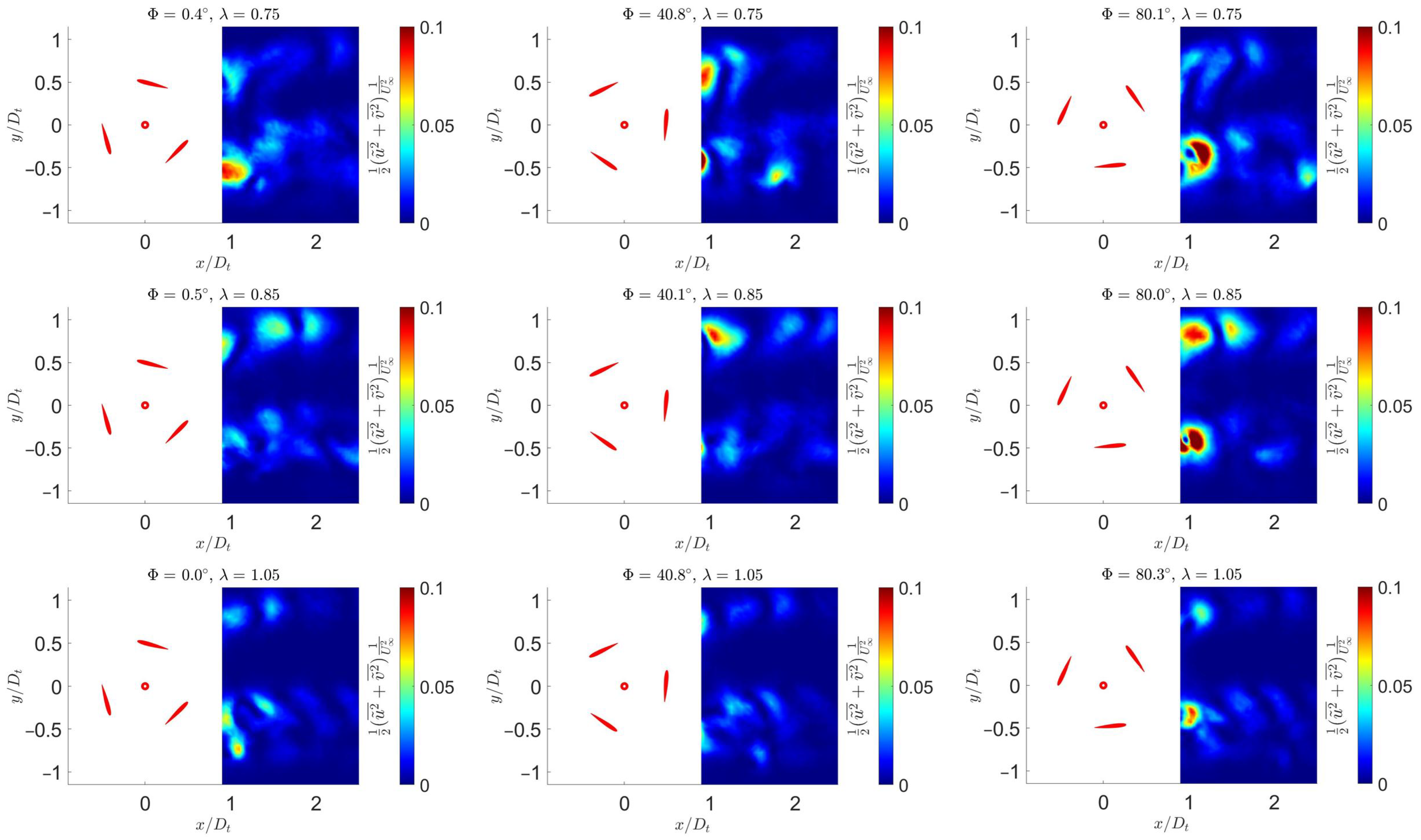
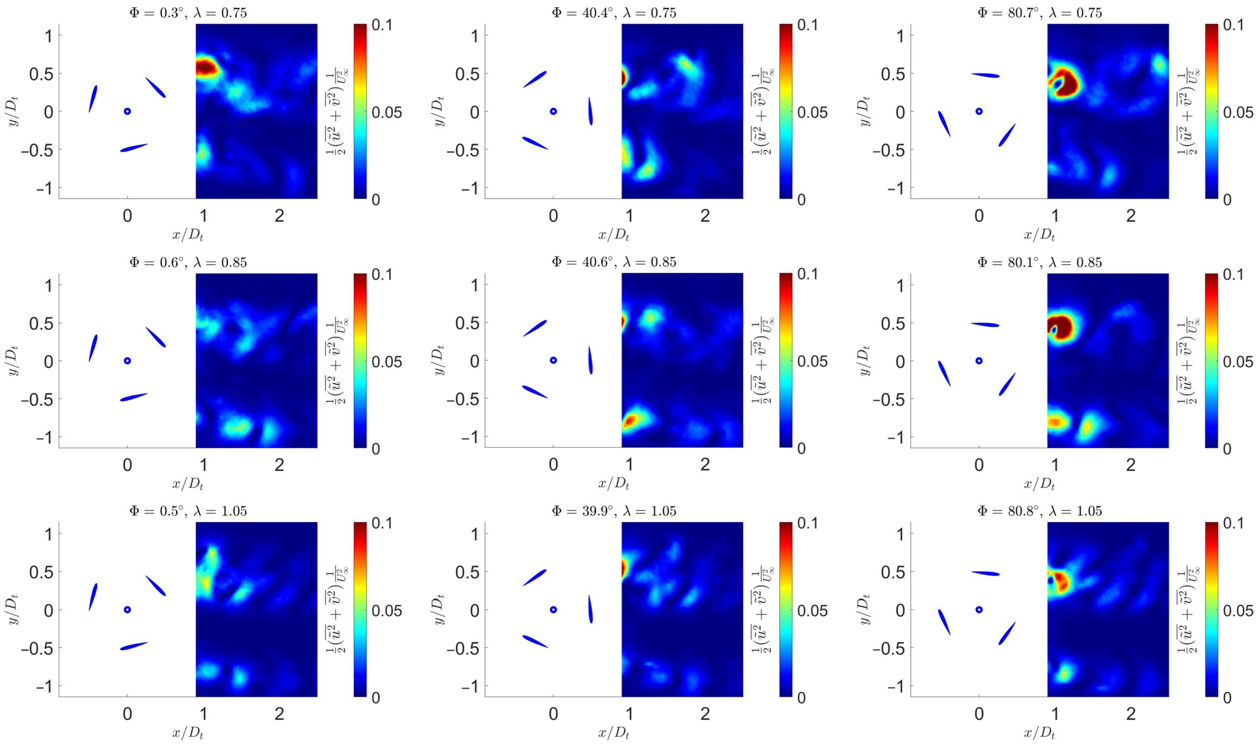
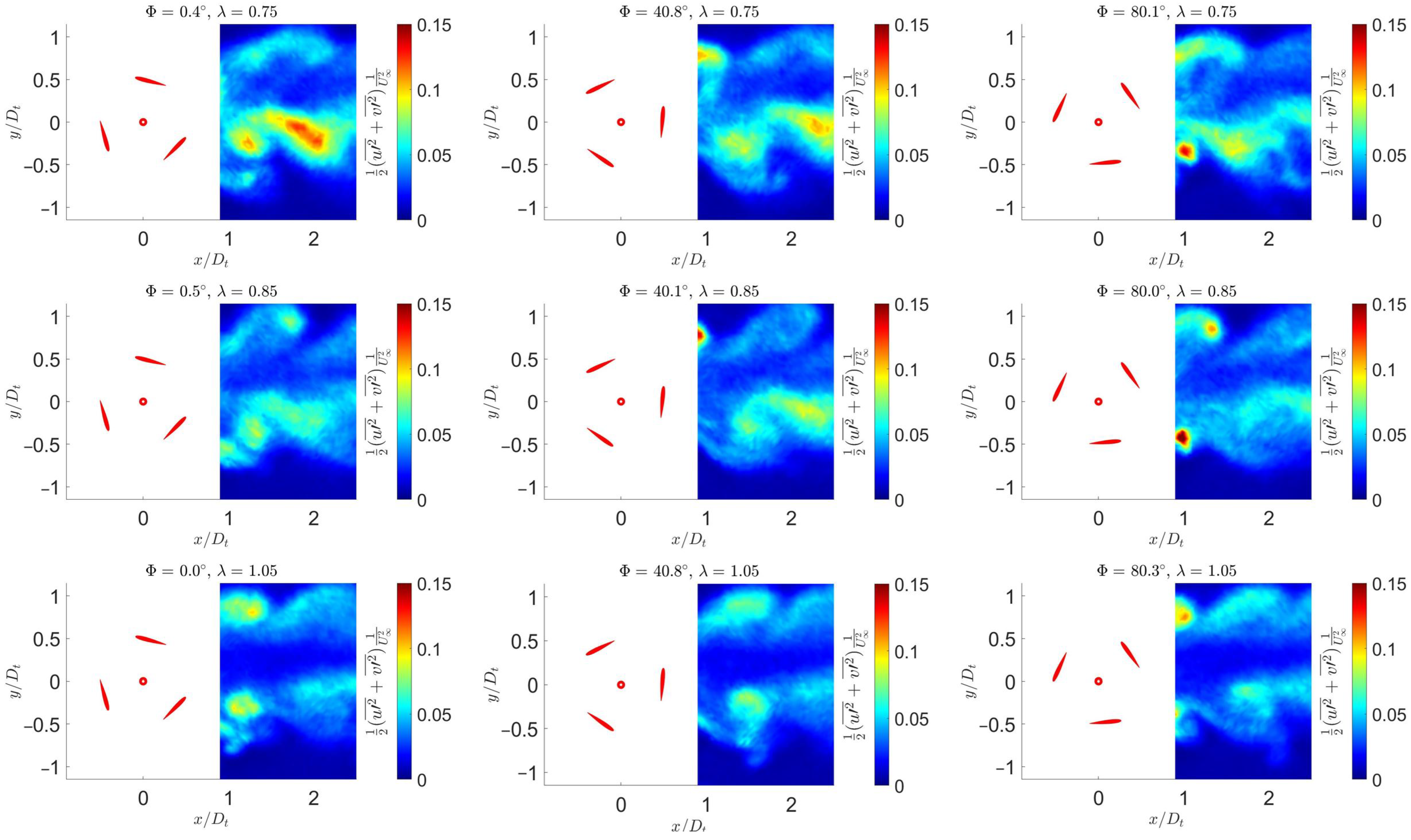
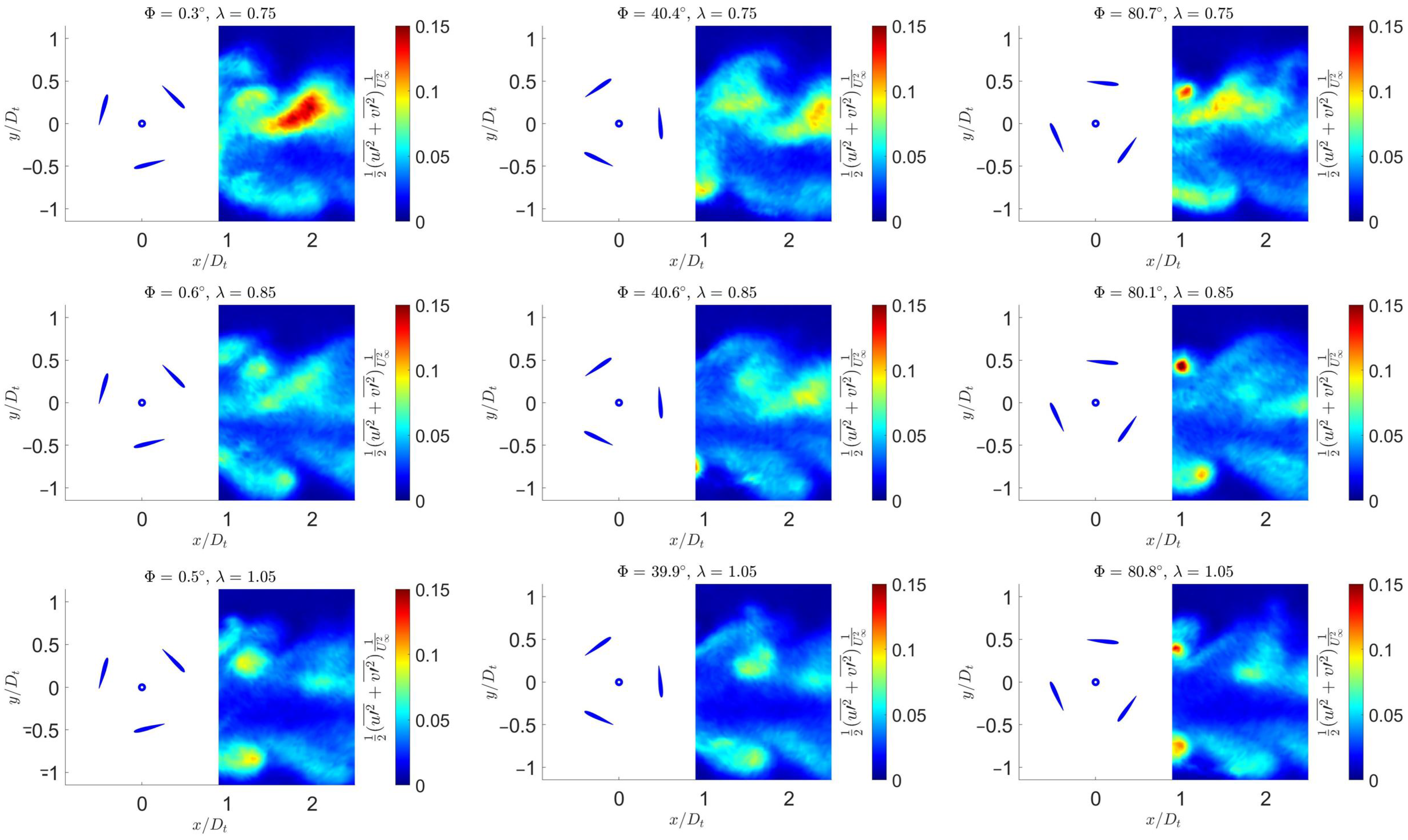
where the velocity components are defined by Equations (1) and (2). Although phase-averaging the random velocity components results in zero, the phase-averaged random kinetic energy, which depends on the squared velocities, represents part of the fluid energy loss. While the mean kinetic energy component, shown in Figure 14, could be computed directly from the associated mean velocity field, the other two terms required further post-processes. To calculate the phase-dependent K ˜ ( Φ ) and K ( Φ ) terms, each velocity component was first phase-averaged with the frequency of 3 f t as suggested by the above FFT analysis. Then, all the periodic and random components of the velocity (Equations (1) and (2)) and kinetic energy (Equations (4) and (5)) at the three turbine speeds were calculated and plotted in Figure 15, Figure 16, Figure 17 and Figure 18.
By qualitatively looking at individual turbines, a direct correlation between the output power and mean kinetic energy in the wake could be observed in Figure 14. For λ < 1 , increasing the turbine rotational speed expanded the slow (low kinetic energy) region behind the turbine and minimally energized the flow on the sides. At λ > 1 , the slow region was smaller, while the fluid accelerated faster on the sides compared to the other two cases. On the other hand, increasing the speed also decreased the amount of energy loss due to the periodic and random component (Figure 15, Figure 16, Figure 17 and Figure 18).

3.5. Quantitative Evaluation

For all of the contour plots of different parameters except for the mean velocity streamlines, turbine T1 and T2 show symmetrical images, and no obviously significant difference was observed. The energy random component plots (Figure 17 and Figure 18) even indicated that T2 created slightly more energy loss in its wake due to the random component, while T2 was experimentally shown to produce more output power compared to T1. As a consequence, the results needed deeper analyses for detailed comparison between the turbines. All the kinetic energy components were first extracted at the fixed streamwise location of x / D t = 1.0 for the entire width of the PIV window and numerically evaluated by
P K ¯ ( x = 1 ) = 1 | y 2 y 1 | y = y 1 y 2 K ¯ ( x = 1 , y ) d y ,
P K ˜ ( x = 1 ) = 1 T t = 0 T 1 | y 2 y 1 | y = y 1 y 2 K ˜ ( x = 1 , y ) d y d t ,
P K ( x = 1 ) = 1 T t = 0 T 1 | y 2 y 1 | y = y 1 y 2 K ( x = 1 , y ) d y d t ,
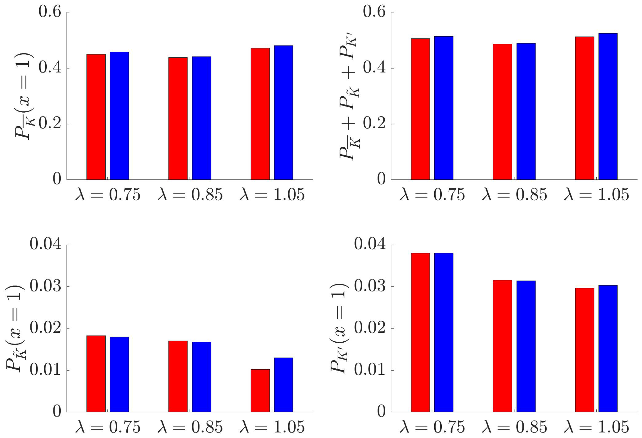
where P K ¯ , P K ˜ , and P K are the representative averaged power over time and space at x / D t = 1.0 , y 1 and y 2 are the limits of the PIV window (in the vertical direction), and T is one third of the turbine period at the relevant speed. The integrated results are summarized in Figure 19, which shows that the fluid power losses were mainly due to the mean component. More interestingly, the loss due to the random component are about twice the loss due to the fluctuating component. The sum of all the losses in Figure 19, once again, proved that the kinetic energy loss is directly correlated with the power production for each turbine. Comparing the two turbines, T2 not only produced more power output but also slightly more losses in its wake. Although the limitation of these experiments is that results are purely two dimensional, the three dimensionality of each configuration can be seen with the numerical divergence of the velocity field. Using the 2D divergence of the velocity
D = u ¯ x + v ¯ y ,
the averaged divergence at x / D t = 1.0 can be evaluated, similar to the kinetic energy above, as
D ¯ ( x = 1 ) = 1 | y 2 y 1 | y = y 1 y 2 | D ( x = 1 , y ) | d y .
The result of this divergence calculation is shown in Table 1, which indicates stronger third-dimensional flow components of turbine T2.

4. Conclusions

This article presented experimental fluid flow results of the near wake region of two independent marine hydrokinetic turbines (T1 and T2) as an extension of the previous power measurement experiment. By using a monoscopic particle image velocimetry technique, the wakes of the turbines were observed to be qualitatively similar with minor deviations from each other due to imperfections in the manufacturing and assembly processes. Moreover, conducting the measurements with three rotational speeds and two independent turbines allowed the observation of the correlation between the turbine power production and the fluid flow structures behind them.
For each individual turbine, lower turbine power output cases with more kinetic energy losses in the wake created more strongly skewed streamlines of the fluid velocity fields. Further decomposition of the kinetic energy losses suggested that the turbine operating at its optimal tip–speed ratio produced the least amount of mean kinetic energy component in the wake. Compared to T1, turbine T2 produced more power output and at the same time more kinetic energy loss while exhibited enhancement of the flow in the third dimension.
This study lay a foundation for future wake measurements of T1 and T2 in counter-rotating configurations. Part II presents the flow results of six different counter-rotating configurations including different separation distances, relative free-stream flow directions, and phase-angle differences. While these turbines will not be geometrically scalable for industrial applications, the physics behind their power production stays valuable and relevant for turbine designers and engineers in the future.

Author Contributions

Conceptualization, M.N.D. and S.O.; methodology, M.N.D. and Y.K.; software, M.N.D. and Y.K.; validation, M.N.D. and Y.K.; formal analysis, M.N.D. and T.K.; investigation, M.N.D., T.K., and Y.K.; resources, S.O.; data curation, M.N.D.; writing—original draft preparation, M.N.D. and S.O.; writing—review and editing, S.O.; visualization, M.N.D.; supervision, T.K. and S.O.; project administration, S.O.; funding acquisition, S.O. All authors have read and agreed to the published version of the manuscript.

Funding

This research received no external funding.

Institutional Review Board Statement

Not applicable.

Informed Consent Statement

Not applicable.

Data Availability Statement

Raw data can be retrieved by private communication with the correpondence.

Acknowledgments

M.N.D. thanks Ivan Alayeto, Kana Kumazawa, Claudio Padricelli, Keita Ando, Uros Markovic, Naomichi Baba, Naoya Sumimura, Julio Barros, Anna Mizobuchi, Mehdi Badri, and Laura Beninati for fruitful discussions and help with the experimental setup. The authors also thank Hisae Mizuno for her endless help with the grant and logistics paperwork. This research was partly supported by the Keio Design The Future award and the Keio Leading-Edge Laboratory of Science and Technology Grant.

Conflicts of Interest

The authors declare no conflict of interest.

Abbreviations

The following abbreviations are used in this manuscript:
MHKMarine hydrokinetic turbine
EDMElectrical discharge machining
VAWTVertical axis wind turbine
LDVLaser Doppler velocimetry

References

  1. Bahar, H. Renewables 2020—Analysis and Forecast to 2025; Report; International Energy Angency: Paris, France, 2020; Available online: https://www.iea.org/reports/renewables-2020 (accessed on 28 March 2021).
  2. Narune, A.; Prasad, E. Renewable Energy Market by Type (Hydroelectric Power, Wind Power, Bioenergy, Solar Energy, and Geothermal Energy), and End Use (Residential, Commercial, Industrial, and Others): Global Opportunity Analysis and Industry Forecast, 2018–2025; Report EN 17140; Allied Market Research: Portland, OR, USA, 2019. [Google Scholar]
  3. Wu, J.; Huang, J.; Han, X.; Xie, Z.; Gao, X. Ecology: Three-Gorges dam experiment in habitat fragmentation? Science 2003, 300, 1239–1240. [Google Scholar] [CrossRef]
  4. Jackson, S.; Sleigh, A. Resettlement for China’s Three Gorges Dam: Socio-economic impact and institutional tensions. Communist Post Commun. Stud. 2000, 33, 223–241. [Google Scholar] [CrossRef]
  5. Tilt, B.; Braun, Y.; He, D. Social impacts of large dam projects: A comparison of international case studies and implications for best practice. J. Environ. Manag. 2009, 90, S249–S257. [Google Scholar] [CrossRef]
  6. Dabiri, J. Potential order-of-magnitude enhancement of wind farm power density via counter-rotating vertical-axis wind turbine arrays. J. Renew. Sustain. Energy 2011, 3, 043104. [Google Scholar] [CrossRef] [Green Version]
  7. Brownstein, I.D.; Wei, N.J.; Dabiri, J.O. Aerodynamically Interacting Vertical-Axis Wind Turbines: Performance Enhancement and Three-Dimensional Flow. Energies 2019, 12, 2724. [Google Scholar] [CrossRef] [Green Version]
  8. Jiang, Y.; Zhao, P.; Stoesser, T.; Wang, K.; Zhou, L. Experimental and numerical investigation of twin vertical axis wind turbines with a deflector. Energy Convers. Manag. 2020, 209, 112588. [Google Scholar] [CrossRef]
  9. Li, Y.; Calisal, S. Modeling of twin-turbine systems with vertical axis tidal current turbines: Part 1—Power Output. Ocean. Eng. 2010, 37, 627–637. [Google Scholar] [CrossRef]
  10. Li, Y.; Calisal, S. Modeling of twin-turbine systems with vertical axis tidal current turbine: Part 2—Torque Fluctuation. Ocean. Eng. 2011, 38, 550–558. [Google Scholar] [CrossRef]
  11. Bachant, P.; Wosnik, M. Performance measurements of cylindrical- and spherical-helical cross-flow marine hydrokinetic turbines, with estimates of exergy efficiency. Renew. Energy 2014, 74, 318–325. [Google Scholar] [CrossRef]
  12. Bachant, P.; Wosnik, M.; Gunawan, B.; Neary, V. Experimental study of a reference model vertical-axis cross-flow turbine. PLoS ONE 2016, 11, e0163799. [Google Scholar] [CrossRef] [Green Version]
  13. Bachant, P.; Wosnik, M. Effects of Reynolds number on the energy conversion and near-wake dynamics of a high solidity vertical-axis cross-flow turbine. Energies 2016, 9, 73. [Google Scholar] [CrossRef] [Green Version]
  14. Strom, B.; Brunton, S.; Polagye, B. Intracycle angular velocity control of cross-flow turbines. Nat. Energy 2017, 2, 17103. [Google Scholar] [CrossRef]
  15. Bachant, P.; Wosnik, M. Modeling the near-wake of a vertical-axis cross-flow turbine with 2-D and 3-D RANS. J. Renew. Sustain. Energy 2016, 8, 053311. [Google Scholar] [CrossRef] [Green Version]
  16. Mannion, B.; Leen, S.; Nash, S. A two and three-dimensional CFD investigation into performance prediction and wake characterisation of a vertical axis turbine. J. Renew. Sustain. Energy 2018, 10, 034503. [Google Scholar] [CrossRef]
  17. Mannion, B.; McCormack, V.; Leen, S.; Nash, S. A CFD investigation of a variable-pitch vertical axis hydrokinetic turbine with incorporated flow acceleration. J. Ocean. Eng. Mar. Energy 2019, 5, 21–39. [Google Scholar] [CrossRef] [Green Version]
  18. Mannion, B.; McCormack, V.; Kennedy, C.; Leen, S.; Nash, S. An experimental study of a flow-accelerating hydrokinetic device. Proc. Inst. Mech. Eng. Part J. Power Energy 2018, 1, 148–162. [Google Scholar] [CrossRef] [Green Version]
  19. Ross, H.; Polagye, B. An experimental assessment of analytical blockage corrections for turbines. Renew. Energy 2020, 152, 1328–1341. [Google Scholar] [CrossRef] [Green Version]
  20. Araya, D.; Colonius, T.; Dabiri, J. Transition to Bluff-Body Dynamics in the Wake of Vertical-Axis Wind Turbines. J. Fluid Mech. 2017, 813, 346–381. [Google Scholar] [CrossRef] [Green Version]
  21. Doan, M.N.; Alayeto, I.H.; Padricelli, C.; Obi, S.; Totsuka, Y. Experimental and computational fluid dynamic analysis of laboratory-scaled counter-rotating cross-flow turbines in marine environment. In Proceedings of the ASME 2018 5th Joint US-European Fluids Engineering Division Summer, Montreal, QC, Canada, 15–20 July 2018; American Society of Mechanical Engineer: New York, NY, USA, 2018; Volume 2, p. V002T14A003. [Google Scholar]
  22. Doan, M.N.; Alayeto, I.H.; Kumazawa, K.; Obi, S. Computational fluid dynamic analysis of a marine hydrokinetic crossflow turbine in low Reynolds number flow. In Proceedings of the ASME-JSME-KSME 2019 8th Joint Fluids Engineering, San Francisco, CA, USA, 28 July–1 August 2019; American Society of Mechanical Engineer: New York, NY, USA, 2019; Volume 2, p. V002T02A067. [Google Scholar]
  23. Alayeto, I.H.; Doan, M.N.; Kumazawa, K.; Obi, S. Wake characteristics comparison between isolated and pair configurations of marine hydrokinetic crossflow turbines at low Reynolds numbers. In Proceedings of the ASME-JSME-KSME 2019 8th Joint Fluids Engineering, San Francisco, CA, USA, 28 July–1 August 2019; American Society of Mechanical Engineer: New York, NY, USA, 2019; Volume 1, p. V001T01A037. [Google Scholar]
  24. Markovic, U.V. Characterizing the Wake and the Performance of a Marine Hydrokinetic Turbine in a Tandem Array Configuration. Master’s Thesis, Bucknell University, Lewisburg, PA, USA, 2016. [Google Scholar]
  25. Doan, M.; Kai, Y.; Obi, S. Twin Marine Hydrokinetic Cross-Flow Turbines in Counter Rotating Configurations: A Laboratory-Scaled Apparatus for Power Measurement. J. Mar. Sci. Eng. 2021, 8, 918. [Google Scholar] [CrossRef]
  26. Lust, E.; Flack, K.; Luznik, L. Survey of the near wake of an axial-flow hydrokinetic turbine in quiescent conditions. Renew. Energy 2018, 129, 92–101. [Google Scholar] [CrossRef]
  27. Araya, D.; Dabiri, O. A comparison of wake measurements in motor-driven and flow-driven turbine experiments. Exp. Fluids 2015, 56, 150. [Google Scholar] [CrossRef]
  28. Suryadi, A.; Ishii, T.; Obi, S. Stereo PIV measurement of a finite, flapping rigid plate in hovering condition. Exp. Fluids 2010, 49, 447–460. [Google Scholar] [CrossRef]
  29. Suryadi, A. The Phase-Avreaged Velocity Measurement and the Estimation of Pressure Force of a Periodically Moving Body. Ph.D. Thesis, Keio University, Yokohama, Japan, 2011. [Google Scholar]
  30. MathWroks. Fast Fourier Transform. Available online: https://www.mathworks.com/help/matlab/ref/fft.html (accessed on 28 March 2021).
  31. Antonia, R.; Bisset, D.; Browne, L. Effect of Reynolds number on the topology of the organized motion in a turbulent boundary layer. J. Fluid Mech. 1990, 213, 267–286. [Google Scholar] [CrossRef]
  32. Kim, H.; Kline, S.; Reynolds, W. The production of turbulence near a smooth wall in a turbulent boundary layer. J. Fluid Mech. 1971, 15, 133–160. [Google Scholar] [CrossRef]
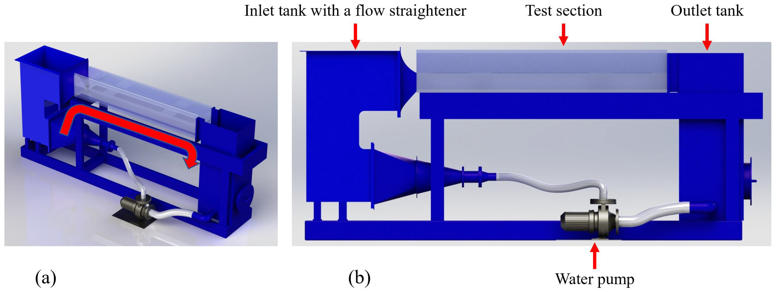
Figure 1. A 3D illustration (a) and side-view (b) of the flume facility with its main components. The red arrow on the left picture indicates the water flow direction.
Jmse 09 00489 g001
Figure 2. Pictures of the apparatus in action: a single turbine inside the water channel (a), a laser sheet illuminates seeding particles behind the turbine (b), and a raw PIV picture (c).
Jmse 09 00489 g002
Figure 3. A rendered picture of the turbine apparatus (a) and its critical mechanical and electronic components (b).
Jmse 09 00489 g003
Figure 4. An overview of the monoscopic particle image velocimetry setup.
Jmse 09 00489 g004
Figure 5. An illustration of the turbine configurations studied in this article: Turbine T1 (a) and Turbine T2 (b). The regions of interest are enclosed inside the red dashed lines, and the arbitrary points for time-series data extraction are highlighted with the 4 red circles inside the dashed lines.
Jmse 09 00489 g005
Figure 6. The power curve of each turbine with the flow measurement points highlighted. In the power measurement experiment, turbine T2 stalled at λ = 0.75 [25]. This figure displays a linear extrapolation of T2 C P at λ = 0.75 .
Jmse 09 00489 g006
Figure 7. The FFT analyses of the time series streamwise and transverse velocities at the 4 points, highlighted in Figure 5, in the near-wake of the T1 turbine configuration at λ = 0.75 .
Jmse 09 00489 g007
Figure 8. The FFT analyses of the time series streamwise and transverse velocities at the 4 points, highlighted in Figure 5, in the near-wake of the T2 turbine configuration at λ = 1.05 .
Jmse 09 00489 g008
Figure 9. An example of the flow converged over more than 100 phases of the T1 configuration at λ = 0.85 and at Φ = 71 . The vertical axes are the streamwise and transverse velocities, at the 4 points highlighted in Figure 5, averaged over time.
Jmse 09 00489 g009
Figure 10. An example of the flow converged over more than 100 phases of the T2 configuration at λ = 0.85 and at Φ = 13 . 6 . The vertical axes are the streamwise and transverse velocities, at the 4 points highlighted in Figure 5, averaged over time.
Jmse 09 00489 g010
Figure 11. The time-averaged non-dimensionalized velocity and vorticity of the T1 configuration at λ = 0.75 (a), λ = 0.85 (b), and λ = 1.05 (c) with the associated power coefficients. The red circle displays turbine T1 rotation center.
Jmse 09 00489 g011
Figure 12. The time-averaged non-dimensionalized velocity and vorticity of the T2 configuration at λ = 0.75 (a), λ = 0.85 (b), and λ = 1.05 (c) with the associated power coefficients. The blue circle displays turbine T2 rotation center.
Jmse 09 00489 g012
Figure 13. The streamwsie velocity component of turbine T1 (a) and T2 (b) at the 3 tip–speed ratios and 4 streamwise locations.
Jmse 09 00489 g013
Figure 14. The time -averaged kinetic energy of the flow behind turbine T1 (a) and turbine T2 (b). The red circle displays turbine T1 rotation center, while the blue circle displays turbine T2 rotation center.
Jmse 09 00489 g014
Figure 15. The fluctuating component of the phase-averaged kinetic energy of the flow behind turbine T1 at various phase angles and tip–speed ratios. The red circle displays turbine T1 rotation center.
Jmse 09 00489 g015
Figure 16. The fluctuating component of the phase-averaged kinetic energy of the flow behind turbine T2 at various phase angles and tip–speed ratios. The blue circle displays turbine T2 rotation center.
Jmse 09 00489 g016
Figure 17. The random component of the phase-averaged kinetic energy of the flow behind turbine T1 at various phase angles and tip–speed ratios. The red circle displays turbine T1 rotation center.
Jmse 09 00489 g017
Figure 18. The random component of the phase-averaged kinetic energy of the flow behind turbine T2 at various phase angles and tip–speed ratios. The blue circle displays turbine T2 rotation center.
Jmse 09 00489 g018
Figure 19. Summary of the kinetic energy components of turbine T1 (red) and T2 (blue) at x / D t = 1.0 averaged over space and time.
Jmse 09 00489 g019
Table 1. Comparison of each configuration temporally and spatially averaged divergence at x / D t = 1.0 .
λ D ¯ ( x = 1 ) T1 D ¯ ( x = 1 ) T2
0.750.2850.312
0.850.2320.247
1.050.3180.328
Publisher’s Note: MDPI stays neutral with regard to jurisdictional claims in published maps and institutional affiliations.