Motion Pattern Optimization and Energy Analysis for Underwater Glider Based on the Multi-Objective Artificial Bee Colony Method

Abstract

Underwater gliders are prevailing in oceanic observation nowadays for their flexible deployment and low cost. However, the limited onboard energy constrains their application, hence the motion pattern optimization and energy analysis are the key to maximizing the range of the glider while maintaining the acceptable navigation preciseness of the glider. In this work, a Multi-Objective Artificial Bee Colony (MOABC) algorithm is used to solve the constrained hybrid non-convex multi-objective optimization problem about range and accuracy of gliders in combination with specific glider dynamics models. The motion parameters Pareto front that balances the navigational index referring to range and preciseness are obtained, relevant gliding profile motion results are simulated simultaneously, and the results are compared with the conventional gliding patterns to examine the quality of the solution. Comparison shows that, with the utilization of the algorithm, glider voyage performance with respect to endurance and preciseness can be effectively improved.

1. Introduction

Underwater gliders have become an important ocean observing platform based on characteristics of low cost, long duration, and flexible mobility, etc. [1,2,3]. Gliders are designed to achieve three-dimensional motion by the buoyancy-driven system, which significantly reduces the navigational energy consumption [4]. However, without any powerful thruster, once gliders are not surfaced receiving the satellite signal to correct the course for a long time, the gliding state will be severely disturbed by the marine environment. In view of such design, the optimization of motion pattern and energy analysis for enhancing the navigation range as well as improving the navigation accuracy have long been the focus of research [5].

Regarding motion optimization of the glider with separate navigational objectives, a lot of excellent research has been carried out: Zamud et al. introduce their work on utilizing the Differential Evolution (DE) algorithm to optimize a series of departure points bearing angles to counteract the effects of ocean currents and make the glider reach the predetermined waypoint accurately [6]. Song et al. construct a precise energy consumption model and gliding range model of the underwater glider; based on the established model, the optimal gliding range of underwater gliders increases 11.97% with an average diving depth of 1000 m [7]. By applying the CTS-A* algorithm, Zhou et al. conducted the path planning with adjustable gliding speed under ocean current information, which can significantly improve the gliding efficiency [8].

However, it is difficult to meet the diversity requirements of actual observation missions by optimizing only a single gliding movement objective. In addition, different navigational indexes could cause mutually-restrictive control requirements, thus the multi-objective path planning of gliders needs to be considered. For the multiple objective glider motion optimization: Enrique et al. proposed an iterative optimization algorithm that can solve navigation accuracy and endurance problems [9]; however, the accuracy of gliding movement was studied under the constraints of fixed time; correspondingly, the problem of the gliding endurance was studied under the premise of fixed distance, which didn’t involve comprehensive decision-making of multi-index combination in path planning. Shadden et al. constructed energy consumption and time-consuming weights functions of gliding motion to optimize glider performance in dynamic ocean currents [5], but the acquisition of the optimal solution is largely dependent on the selection of the weight coefficients; thus, it was difficult to examine whether the obtained solutions are the optimal result for each objective combination.

The artificial bee colony algorithm is a heuristic swarm intelligence optimization algorithm based on the simulation of the bee colonies foraging process.The algorithm implements optimization by imitating the information interaction between bees, which was first proposed by Karaboga [10]. With the random search on the solution space and the mutual role transformation among the employed bees, the onlooker bees and the scout bees, the algorithm not only has a good local search ability, but also has a global search ability. For the multi-objective optimization, Ref. [11] proposed the multi-objective artificial bee colony algorithm with a grid based approach for maintaining the external archive, and the method can effectively solve the multi-objective optimization problems. In [12], a non-dominated sorting based multi-objective artificial bee colony algorithm is proposed; the proposed methods have been compared with NSGA-II [13], MOVGA, and it verifies the effectiveness in solving multi-objective problems. With the excellent Pareto optimization performance, the MABC algorithm has been widely used in many fields [14,15,16,17].

There are few studies on the multi-objective optimization of glider motion using MABC at present; this is because the model can completely simulate the motion process of a glider that needs to be studied. In [18], the dynamic model of glider adopts conventional AUV and a hydrodynamic model of submarines. In [19], the glider model that steered by a single internal movable and rotatable mass is established, and the steady spiral movement of the glider is analyzed. However, these models all simplify the motion process of the glider, and do not consider the coupled motion characteristics of six degrees of freedom, so they cannot accurately reflect the motion characteristics of the glider, which poses a challenge for the optimization of motion.

In this work, we choose the preciseness of trajectories and range of gliders as motion objectives to evaluate the navigational quality. The main contribution lies in the establishment of the full-process dynamics model of the glider, combined with the advanced updated MABC algorithm of Pareto, in order to optimize the motion of the glider to simultaneously ensure a long range and accurate fitting to the preset trajectory.

The paper is organized as follows: Section 2 derives the glider dynamic model; Section 3 presents the motion pattern and energy analysis of the glider; Section 4 introduces MABC. Section 5 exhibits the numerical simulation results and experiments’ discussion. Finally, conclusions are summarized.

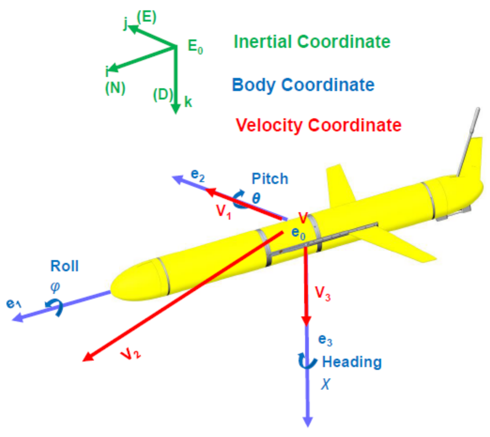
2. Underwater Glider Dynamic Modeling

The underwater glider studied in this paper is equipped with sonar, CTD, and current meter to observe the ocean environment. Figure 1 shows the overall structure of the underwater glider, in which the main regulating mechanism is located in the pressure sealed cabin shown in Figures A and B, which are buoyancy adjusting unit and attitude control unit, respectively. The attitude control of the glider can be realized by changing the position of the battery pack, which can move axially and rotate around the axis, thus causing the change of the overall center of gravity. The glider heave control is realized by changing the amount of oil in the internal buoyancy adjusting unit to change the overall net buoyancy.The glider’s course and trajectory can be controlled by controlling the change of attitude and net buoyancy and combining with the hydrodynamics generated by the wing.The specific parameters of this type of glider are shown in Nomenclature.

Dynamic modeling is the premise of dynamic analysis and algorithm control of underwater gliders. This chapter adopts the conventional Lagrange dynamic equation method, which is used to study the motion characteristics of gliders in three coordinate systems. Firstly, the force analysis is carried out in the inertial coordinate system, and then the equivalent relation is established through the conservation of energy and momentum. Finally, the hydrodynamic analysis results are converted into the above equivalent relation, in order to establish a complete dynamic model.

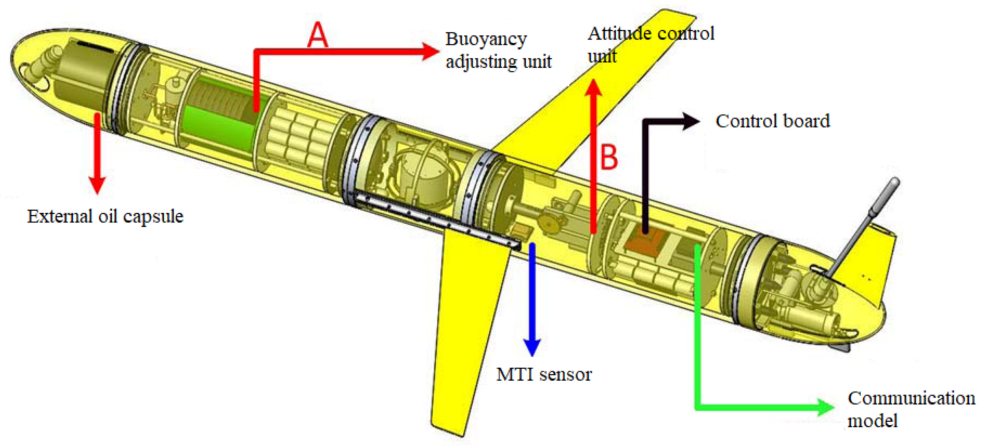
2.1. Model Derivations

There are three coordinate systems: inertial coordinate system, body coordinate system, and velocity coordinate system. Inertial coordinate system ${\mathit{E}}_{\mathbf{0}}(\mathit{i},\mathit{j},\mathit{k})$: In the inertial coordinate system, the force status of the object can be clearly expressed. $E_0$ is a point in space, $\mathit{i}$ is north, $\mathit{j}$ is east, and $\mathit{k}$ is vertically downward. Body coordinate system ${\mathit{e}}_{\mathbf{0}}({\mathit{e}}_{\mathbf{1}},{\mathit{e}}_{\mathbf{2}},{\mathit{e}}_{\mathbf{3}})$ is established at the buoyancy center of the glider, ${\mathit{e}}_{\mathbf{1}}$ is the axis direction of the glider, pointing to the front; ${\mathit{e}}_{\mathbf{2}}$ lies in the wing plane, pointing to the right; ${\mathit{e}}_{\mathbf{3}}$ is selected as ${\mathit{e}}_{\mathbf{1}}\times {\mathit{e}}_{\mathbf{2}}$.The angles corresponding to the glider rotation around the body coordinate axes are Roll, Pitch, and Heading, respectively. The general diagram about coordinate systems are shown in Figure 2.

Glider mass can be divided into three parts in the analysis of glider mechanics: the glider fixed part ($rb$), the battery pack part ($mr$), and the buoyancy adjustment part (b). The mass of these three parts and their distances from the origin point $e_0$ of the body coordinate system are represented by symbol m and r, respectively.

The momentum and momentum moment expression formula of glider system and movable battery pack in the inertial coordinate system are as Equation (1):

$$\mathit{\tau }=\left[\begin{array}{c}P\\ \pi \\ p_{mr}\\ {\pi }_{mr}\end{array}\right],\mathit{\eta }=\left[\begin{array}{c}{R}_{EB}P\\ R_{EB}\Pi +b\times p\\ R_{EB}{P}_{mr}\\ R_{EB}{\Pi }_{mr}+b\times p_{mr}\end{array}\right]$$

(1)

Differentiate $\tau$ with respect to time to obtain the generalized force in the inertial frame, the specific expression form as Equations (2)–(5):

$$\frac{\mathrm{d}\mathit{p}}{\mathrm{d}t}=(m_{mr}+m_{rb}+m_b-m)g\mathit{k}+\sum _{i=1}^I{\mathit{f}}_{exti}$$

(2)

$$\frac{\mathrm{d}\pi }{\mathrm{d}t}=\sum _{i=1}^I{\mathit{x}}_{\mathit{i}}{\mathit{f}}_{exti}+{\mathit{p}}_{\mathit{mrE}}\times m_{mr}g\mathit{k}+{\mathit{p}}_{\mathit{rbE}}\times m_{rb}g\mathit{k}+{\mathit{p}}_{\mathit{bE}}\times m_{b}g\mathit{k}+\sum _{j=1}^J{\mathit{\tau }}_{extj}$$

(3)

$$\frac{\mathrm{d}{\mathit{p}}_{\mathit{mr}}}{\mathrm{d}t}=m_{mr}g\mathit{k}+\sum _{k=1}^K{\mathit{f}}_{intk}$$

(4)

$$\frac{\mathrm{d}{\pi }_{\mathit{mr}}}{\mathrm{d}t}=\sum _{k=1}^K{y}_k\times {\mathit{f}}_{\mathit{intk}}+{\mathit{p}}_{\mathit{mrE}}\times m_{mr}g\mathit{k}+\sum _{s=1}^S{\mathit{\tau }}_{ints}$$

(5)

Similarly, differentiate $\mathit{\eta }$ with respect to time to obtain the generalized force in the body frame, then select the items related to gravity to obtain the force of the glider in the body coordinate system, as shown in Equations (6)–(9):

$$\frac{\mathrm{d}\mathit{P}}{\mathrm{d}t}=P\times \Omega +\overline{m}g\left({\mathit{R}}_{\mathit{EB}}^{\mathit{T}}\mathit{k}\right)+\mathit{F}$$

(6)

$$\frac{\mathrm{d}\Pi }{\mathrm{d}t}=\mathbf{\Pi }\times \mathbf{\Omega }+\mathit{P}\times \mathit{V}+(m_{mr}{r}_{mr}+m_{rb}{r}_{rb}+m_b{r}_b)g\times \left({\mathit{R}}_{\mathit{EB}}^{\mathit{T}}\mathit{k}\right)+\mathit{T}$$

(7)

$$\frac{\mathrm{d}{\mathit{P}}_{\mathit{mr}}}{\mathrm{d}t}={\mathit{U}}_{\mathit{Fmr}}$$

(8)

$$\frac{\mathrm{d}{\Pi }_{\mathit{mr}}}{\mathrm{d}t}={\mathit{U}}_{\mathit{Tmr}}$$

(9)

Next, calculate the total kinetic energy of the glider because we divided it into three parts earlier, plus the water flow damping force. Therefore, the total kinetic energy expression contains four parts, which can be expressed as Equation (10):

$$T=\frac{1}{2}{\mathit{v}}^{\mathit{T}}{\mathit{M}}_{\mathit{rbE}}\mathit{v}+\frac{1}{2}{\mathit{v}}^{\mathit{T}}{\mathit{M}}_{\mathit{mrE}}\mathit{v}+\frac{1}{2}{\mathit{v}}^{\mathit{T}}{\mathit{M}}_{\mathit{bE}}\mathit{v}+\frac{1}{2}{\mathit{v}}^{\mathit{T}}{\mathit{M}}_{\mathit{fE}}\mathit{v}$$

(10)

The first item is the kinetic energy of the battery pack, including the kinetic energy generated by translation and rotation relative to the origin in the body coordinate system. It should be noted that we approximated the mass block to a cylinder of a similar shape during the calculation, and used three-dimensional software to estimate its center of gravity position, so the kinetic energy of the battery pack part is $\frac{1}{2}{m}_{mr}{\mathit{V}}_{\mathit{mr}}^{\mathbf{2}}$. The kinetic energy of the adjustment part is similar to the calculation method of the battery pack, so we will not repeat it here; the value of the last item of water flow resistance mainly depends on the additional mass, additional moment of inertia, and coupling terms. The matrix expression form of each kinetic energy term is given as Equation (11):

$$T_{mr}=\frac{1}{2}{m}_{mr}{\mathit{V}}_{\mathit{mr}}^{\mathbf{2}}+\frac{1}{2}{\mathit{I}}_{\mathit{mr}}\left(\gamma \right){\mathbf{\Omega }}_{\mathit{mr}}^{\mathbf{2}}$$

(11)

Finally, by deriving T for the speed and time, the resultant external force and the resultant external moment of the glider in the dynamic coordinate system can be obtained. The derived model are as Equations (12)–(14):

$$\eta =\frac{\partial T}{\partial v}=Mv$$

(12)

$$\dot{\eta }=\dot{M}v+M\dot{v}$$

(13)

$$\dot{v}=M^{-1}(\dot{\eta }-\dot{M}v)$$

(14)

Through this modeling method, we have obtained the simplified dynamic model of the glider as follows, where F and T are the hydrodynamic force and the corresponding moment of the glider. The solution of these two items will be described in detail in Equation (15):

$$\dot{\mathit{v}}=\left[\begin{array}{c}\dot{\mathit{V}}\\ \dot{\mathbf{\Omega }}\end{array}\right]={\mathit{M}}^{-\mathbf{1}}(\left[\begin{array}{c}\mathit{P}\times \mathbf{\Omega }\\ \mathbf{\Pi }\times \mathbf{\Omega }+\mathit{P}\times \mathit{V}\end{array}\right]+\left[\begin{array}{c}{m}_{b}g\left({\mathit{R}}_{\mathit{EB}}^{\mathit{T}}\mathit{k}\right)\\ (m_{mr}{r}_{mr}+m_{rb}{r}_{rb})g\times \left({\mathit{R}}_{\mathit{EB}}^{\mathit{T}}\mathit{k}\right)\end{array}\right]+\left[\begin{array}{c}\mathit{F}\\ \mathit{T}\end{array}\right]-\dot{\mathit{M}}\mathit{v})$$

(15)

2.2. Hydrodynamic Forces

The hydrodynamic coefficient and additional mass coefficient of the glider are determined by the part of the glider in contact with the water flow. The use of CFD and semi-empirical formulas to calculate its parameters is the premise of its route control later, so this section will introduce in detail how to set up different sailing conditions, and use the least square method to fit 12 hydrodynamic parameters to the simulation results.

In the modeling in the previous section, the hydrodynamic force and hydrodynamic moments received by the underwater glider are represented by ${\mathit{F}}_{\mathit{hy}}$ and ${\mathit{T}}_{\mathit{hy}}$, which include lift, drag, slip force, and the corresponding hydrodynamic moment. The representation of ${\mathit{F}}_{\mathit{hy}}$ and ${\mathit{T}}_{\mathit{hy}}$ in vectors are shown in Equation (16):

$${\mathit{F}}_{\mathit{hy}}=\left[\begin{array}{c}-D\\ SF\\ -L\end{array}\right],{\mathit{T}}_{\mathit{hy}}=\left[\begin{array}{c}{M}_{DL1}\\ M_{DL2}\\ M_{DL3}\end{array}\right]$$

(16)

The use of different hydrodynamic parameters is expressed as Equations (17)–(22):

$$D=(K_{D0}+K_D{\alpha }^2)V^2$$

(17)

$$SF=K_{\beta }\beta$$

(18)

$$L=(K_{L0}+K_t\alpha )V^2$$

(19)

$$M_{DL1}=K_{MR}\beta V^2+K_{p}P{V}^2$$

(20)

$$M_{DL2}=(K_{M0}+K_M\alpha +K_{q}q)V^2$$

(21)

$$M_{DL3}=K_{MY}\beta V^2+K_{r}q{V}^2$$

(22)

For the hydrodynamic coefficients contained in the above expressions, we use the CFD fluid calculation software FLUENT to simulate different angles of attack and sideslip angles, and at the same time establish watersheds of different shapes to simulate different rotational angular speeds. The grids of steady-state gliding and spiral gliding and the quality of these two grids are shown in Figure 3. Based on the past experience of meshing, when the mesh quality is not less than 0.2, we can account that the meshing result is reasonable and the calculation results can be obtained.

$$R_e=\frac{\rho vL}{\mu }$$

(23)

Because the size of the simulation results largely depends on the Reynolds number which is shown in Equation (23), when the temperature is 20 ${}^{\circ }$C, the physical properties of seawater are: $\rho =1.025{\mathrm{kg}/\mathrm{m}}^3$, L = 1.995 m, $\mu /v=1.0785\times {10}^{-6}{\mathrm{m}}^2/\mathrm{s}$; these parameters are used as the boundary conditions of the simulation. The cloud diagrams obtained through hydrodynamic simulation of steady-state gliding and spiral gliding are shown in Figure 4.

In the process of fitting, the independent variables are the angle of attack, the angle of sideslip, and the angular velocity of rotation, and the dependent variables are the forces and moments corresponding to each direction calculated by the software in the body coordinate system. By rotating the matrix ${\mathit{R}}_{\mathit{BC}}$, the lift, drag, sideslip force, and the corresponding hydrodynamic moment can be obtained while using the least square method to fit.

In this way, we use Equations (17)–(22) to correspond to the coefficients of each curve to the hydrodynamic parameters, and then we can get their values as follows:

$K_{D0}=5.5\mathrm{kg}/\mathrm{m},K_D=278.32{\mathrm{kg}/\mathrm{m}/\mathrm{rad}}^2;$

$K_{\beta }=-132.73\mathrm{kg}/\mathrm{m}/\mathrm{rad};$

$K_{L0}=-0.36\mathrm{kg}/\mathrm{m},K_L=440.99\mathrm{kg}/\mathrm{m}/\mathrm{rad};$

$K_{MR}=-65.16\mathrm{kg}/\mathrm{rad},K_P=-21.73\mathrm{kg}·\mathrm{s}/\mathrm{rad};$

$K_{M0}=0.31\mathrm{kg},K_M=-79.72\mathrm{kg}/\mathrm{rad},K_q=-243.01\mathrm{kg}·{\mathrm{s}/\mathrm{rad}}^2;$

$K_{MY}=37.22\mathrm{kg}/\mathrm{rad},K_r=-423.71\mathrm{kg}·{\mathrm{s}/\mathrm{rad}}^2$

3. Motion Pattern and Energy Consumption Analysis

In this section, we discuss the gliding pattern, energy consumption analysis, and heading deficiencies for underwater gliders. The energy consumption of different gliding pattern varies sharply, and it will lead to the accuracy of navigational heading, combined with the derived glider dynamic model; relevant critical problems can be discussed thoroughly.

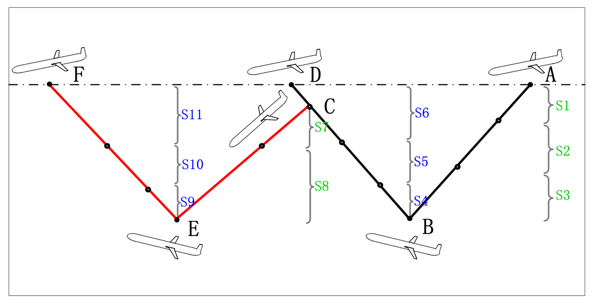
3.1. Motion Pattern Discussion

Generally, motion patterns of glider can be divided as single profile and multi-profile patterns. As shown in Figure 5, where single profiles are presented by the trajectory between A and D, A is the initial point of the diving movement, while D is the communication point on the sea surface after completing a period of profile movement, and B is the state switching point between diving and floating movement. The diving stage A–B can be divided into attitude–buoyancy comprehensive adjustment process, buoyancy adjustment process, and steady state dive stage, as shown as $S1$–$S3$; similarly, the floating stage $BD$ can be divided into attitude–buoyancy adjustment process, buoyancy adjustment process, and steady-state floating process, as shown as $S4$–$S6$. This mode of gliding is widely used by glider navigation due to the convenience of control and high navigational accuracy by frequent communication.

The multi-profile pattern is consistent with the single profile pattern in the A–C section, but, at C point, the floating proceeding will be interrupted and transferred to the submerging procedure, followed by the next cycle movement; this kind of gliding pattern was also called the yo-yo profile in other studies. Compared with the single profile mode, the multi-profile has a huge advantage in energy savings. As the glider body is designed to be negative relative to standard atmospheric pressure, and it uses an electromagnetic valve to precisely control the glider displacement volume of seawater affected by pressure difference between glider internal and external environment, the span of valve operation time is closely related to the energy consumption. Since the C point in a multi-profile pattern is located at a certain depth under the sea surface with a high environmental pressure, the floating-submerging state transition process will complete quickly. In addition, without frequently corresponding on the sea surface, it will reduce the executions of glider posture adjustment actuators. Therefore, when the glider adopts the multi-profile mode, the energy consumption of the system can be effectively reduced. In the next section of our work, we will introduce the energy consumption comparison results of different gliding modes from a quantitative point of view.

3.2. Energy Consumption Analysis

The on-board battery discharge current and discharge time corresponding to each stage of profile are shown in

Table 1. Current and time of battery discharge in each stage of motion.

Stage	I/mA	Time Symbol	Expression
$S_1$	208.8	$t_1$	$\frac{L}{v_m}+(n-1)·T_{{\lambda }_1}$
$S_2$	161.0	$t_2$	$T_{{\lambda }_1}·\frac{\Delta b_1}{B}-t_1$
$S_3$	1.2	$t_3$	$T-t_1-t_2$
$S_4$	356.2	$t_4$	$\xi ·T$
$S_5$	161.0	$t_5$	$\frac{L·n}{v_m}$
$S_6$	1.2	$t_6$	$T_{{\lambda }_2}·\frac{\Delta b_2·n}{B}-t_5$
$S_h$	27.1	$t_7$	$T-t_5-t_6$
$S_{C1}$	185.0	$t_8$	$T_{{\lambda }_2}·\frac{\Delta b_3}{B}$
$S_{C2}$	1.2	$t_9$	$T_{{\lambda }_3}$
$S_{C3}$	1.2	$t_{1}0$	$T_{{\lambda }_4}$

. During the diving phase $S_1$, the electromagnetic valve that allows the external pressure pushes the oil into internal space and the pitch adjustment motor works at the same time; then, during phase $S_2$, the electromagnetic valve continues to work; at $S_3$, the electrical control unit works statically. $S_h$ represents the heading control process, where the roll motor is activated. For the floating stage $S_4$, plunger pump and pitch motor activates at this time, and the plunger pump will continue to work during stage $S_5$; in stage $S_6$, the electrical control unit works statically. $S_h$ represents the heading control process. $S_{C1}$–$S_{C3}$ elaborate the communication between glider and on shore control center; at phase $S_{C1}$, the plunger pump activates to establish the communication attitude; during period $S_{C3}$, the connection establishes and, during period $S_{C2}$, the electrical control unit works statically.

The action time of the glider actuators corresponding to each stage is also listed in Table 1, where L is the totally adjustable distance of center of gravity and $v_m$ refers to the linear velocity of battery pack. $T_{{\lambda }_1}$ is the electromagnetic valve working time; for a fixed floating-diving motion switching depth, the environmental pressure outside the glider can be considered constant, so we assume that $T_{{\lambda }_1}$ is the constant value. $T_{{\lambda }_2}$ is the time for the plunger pump to completely push the oil from the inside of the glider to the external bladder. For the convenience of analysis, the influence of the water pressure on the $T_{{\lambda }_2}$ was neglected, and we considered the plunger pump working on a linear mode; thus, the work time of plunger pump related to any glider buoyancy change can be expressed; T is the time-consuming accumulation of all the dive processes. Since most of the profile motion is in the steady gliding form, it has symmetry in time-consuming accumulation between floating and diving stage.

In addition, let $\xi$ denote the ratio of glider roll angle adjustment motor work time and the total profile time, then the glider heading angle adjustment time can be represented by $\xi ·T$. $T_{{\lambda }_3}$ represents the waiting time before the communication is established and $T_{{\lambda }_4}$ refers to the time of communication.Thus, the power consumption model of the profile mode with different profile numbers n can be formulated as Equation (24):

$$E=\sum I_i·t_i+b,i\in [1,11]$$

(24)

where b is the power consumption of the pitching adjustment motor except for working with electromagnetic valves after the diving-floating switching process, and can be expressed as Equation (25):

$$b=(I_1-I_2)·(\frac{L}{v_m}-T_{{\lambda }_1})$$

(25)

Considering that the battery power carried by the glider is fixed, comparing the power consumption between the single profile mode and multi-profile mode on the premise of completing the same navigation range. Assume that the single-profile case completed the movement by i motion cycles and the multi-profile case j motion cycles, so, by letting $e=E_1-E_n>0$, it can then get $n>2.615$, which implies that, in the vertical plane of gliding motion, when the motion cycles n of multi-profile mode is greater than 3, compared with the single profile form, the glider can consume less power and has higher efficiency when gliding the same distance.

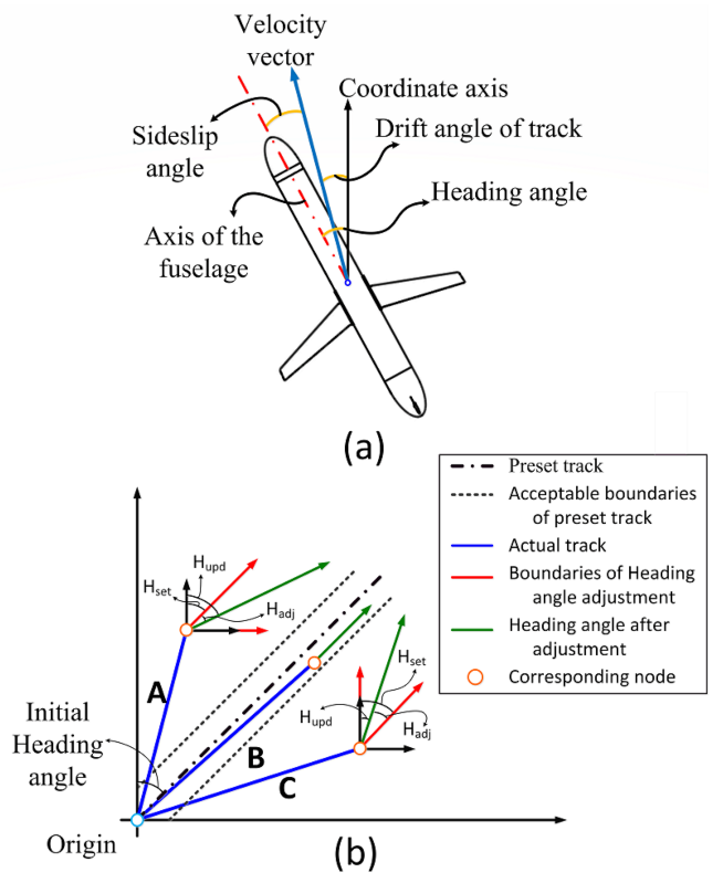
3.3. Discussion of Heading Control Deficiencies on a Horizontal Level

Based on the analysis above, once a larger motion cycle of multi-profile is applied, then it is more beneficial to energy saving. However, taking into account the impact of the marine environment, it is easy to deviate from the target route if gliders do continuous underwater navigation without coming-up on the sea surface to calibrate the route.

Glider heading control is achieved by measuring the Heading angle from the MTI attitude sensor mounted on the interior of glider body. If the axis of the fuselage deviates from the speed vector, a sideslip angle will appear and eventually be off course, as shown in Figure 6a. From our historical sea trial results, the track error of the OUC glider is in the range of 5 to 10 degrees. In this simulation work, we choose the parameter $H_{d}isturb$ to simulate the environmental interfere on the heading control; we also use the parameter $\delta$ to simulate the loss of voyage due to the marine environment interference. In addition, the OUC-III glider angular velocity $\omega \in$ [7 × 10${}^{-3}$, 1.4 × 10${}^{-2}$] rad/s, thus the shifting time from any initial heading angle to the target heading angle is relatively short over the whole profile time (about 2–3 h). For convenience of discussion, the problem of glider motion optimization is simplified in order to maximize the range of glider along a straight line with a minimum yaw error with respect to a predetermined heading angle.

For the existence of the heading error angle, the heading adjustment parameter $H_{a}dj$ is introduced. Figure 6b describes the course adjustment process of the glider in the horizontal plane. Due to the heading error, the track may appear as A, B, or C, which are located outside the acceptable area of the target track in the counterclockwise direction, within the acceptable area and outside the acceptable area in the clockwise direction. The heading adjustment strategy can be expressed as Equation (26):

$$H_{upd}=H_{set}+H_{adj}$$

(26)

where $H_{upd}$ is the adjusted heading angle, and heading angle before adjustment is represented by $H_{set}$. $H_{adj}$ is the heading adjustment angle; it takes the positive value as the optimization parameter, that is, depending on the position of the communication node relative to the target route, and the optimization parameter will take $+H_{adj}$, 0 and $-H_{adj}$. For the convenience of analysis, the following discussion is held within the heading angle scope $[0deg,45deg]$, the other quadrants are under the similar regular.

The course-adjustment angle boundaries of the tracks A and C in Figure 6b are given by the following rules: if the communication node is located counterclockwise outside the acceptable domain, then the original heading is used as the upper bound of the heading adjustment angle, and the heading angle of 90 degrees is used as the lower bound; if the communication node is in the clockwise direction of the acceptable domain, the original heading is used as the lower bound and the heading of 0 degrees is used as the upper bound. At the same time, the upper and lower bounds are both unreachable. Within the boundaries, an optimal angle will be selected by the optimization program as the heading adjustment angle $H_{adj}$.

4. Optimization Problem and Method

This part defines the motion optimization problem of the glider and introduces the corresponding multi-objective artificial bee colony algorithm that can efficiently solve the problem.

4.1. Glider Motion Optimization Problem

In order to indicate the projection of the glider trajectory on the horizontal plane of different motion patterns, the following provisions are defined. Take the glider initial deployment location as the origin point, and take north as the y-axis direction, and east as the x-axis direction to establish the coordinate system with a 1 km unit scale. The coordinates value of each communication node are then as Equations (27) and (28):

$$x\left(i\right)={\delta }_1·s·\sin (H_{set}+H_{disturb}+H_{adj})+x(i-1)$$

(27)

$$y\left(i\right)={\delta }_2·s·\sin (H_{set}+H_{disturb}+H_{adj})+y(i-1)$$

(28)

where s is the distance of single cycle gliding motion, $Depth$ indicates the whole movement depth, and $depth$ indicates the shift motion depth. Then, the target track can be described as Equations (29) and (30):

$$s=\frac{2}{\tan \theta }·[Depth+(n-1)·depth]$$

(29)

$$\tan \theta =\frac{x_g}{y_g}$$

(30)

Then, the acceptable domain of the target track can be defined as the area enclosed by the line pair Equation (31):

$$y_b=\frac{x_b}{\tan H_{set}}\pm \left(1+\frac{1}{{\tan H_{set}}^2}\right)$$

(31)

Defining the distance between the final communication node and the origin was the navigational total range. The sum of the distances of all the communication nodes off the target route was defined as the heading error. We have also taken the ratio between the gliding range and the sum of all cycle gliding distances as the voyage efficiency. Then, we could get the motion indicators as Equations (32)–(34):

$$R=\sqrt{[x{\left(f\right)}^2+x{\left(f\right)}^2]}$$

(32)

$$e=\sum \frac{\mid \frac{1}{\tan H_{set}}·x\left(i\right)+y\left(i\right)\mid }{\sqrt{1+{\left(\frac{1}{\tan H_{set}}\right)}^2}}$$

(33)

$$\eta =\frac{R}{\sum \sqrt{{[x\left(i\right)-x(i-1)]}^2+{[y\left(i\right)-y(i-1)]}^2}}$$

(34)

Hence, the glider motion optimization problem can be represented by the objective function Equation (35):

$$\left\{\begin{array}{cc}\hfill & f_{goal1}=max\left\{R\right\}\hfill \\ \hfill & f_{goal2}=max\left\{e\right\}\hfill \\ \hfill & f_{goal3}=max\left\{\eta \right\}\hfill \end{array}\right.$$

(35)

The restrictions are as Equation (36):

$$\sum E\left(i\right)\le E_{total}$$

(36)

Optimize parameters’ boundaries are as Equation (37):

$$\left\{\begin{array}{cc}\hfill & 1\le n\le 20\hfill \\ \hfill & H_{set}\le \mid H_{adj}\mid \le 90deg,(H_{adj}>0)\hfill \\ \hfill & 0deg\le \mid H_{adj}\mid \le Hset,(H_{adj}<0)\hfill \end{array}\right.$$

(37)

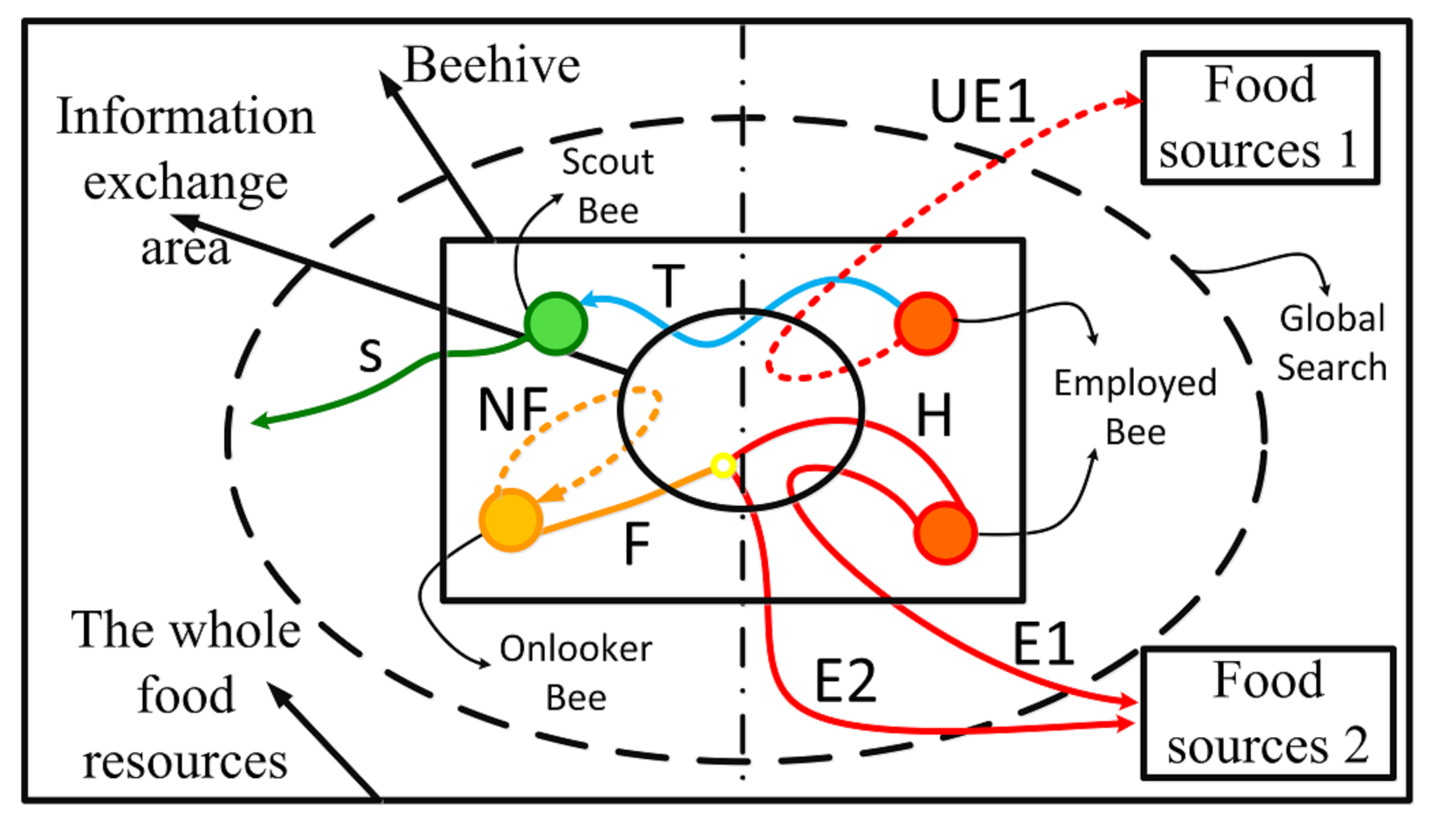
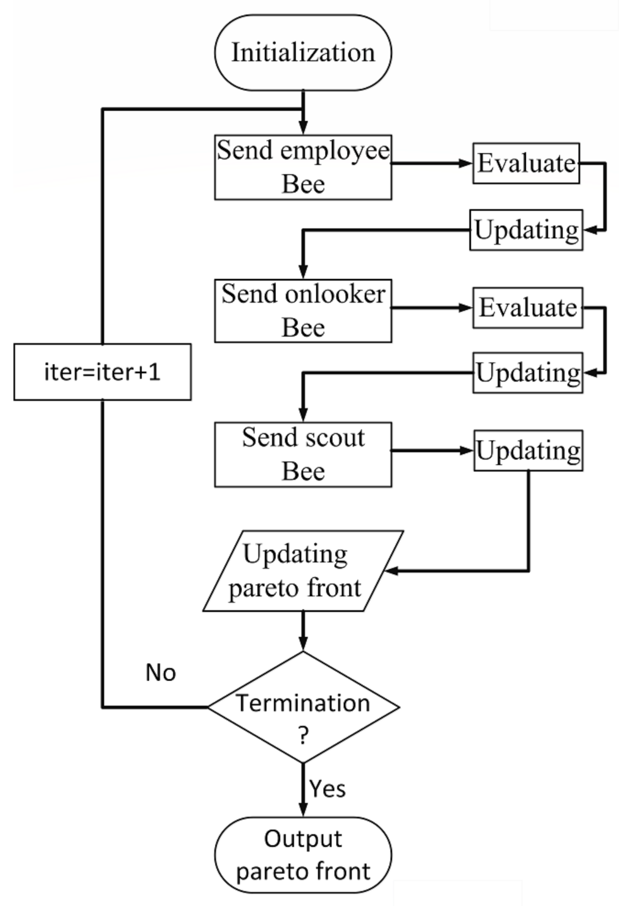
4.2. Multi-Objective Artificial Bee Colony Algorithm

The artificial bee colony algorithm is a heuristic swarm intelligence optimization algorithm based on the simulation of bee colonies foraging process. The algorithm principle is shown in Figure 7. The solution space of the problem corresponds to the food source set. After the initialization, the food source set is divided into the section that will not be explored, and the part that will be explored according to the value of food source (i.e., the quality of the solution). The local optimization process of the algorithm is implemented by the honey collecting behavior of the employed bee and the onlooker bee. Each food source matches an employed bee. During each exploring iteration, the employed bees conduct a random search near the food source. After returning to the information exchange area to share the food source information, they have the following options for the next behavior. The first case is that they will continue to search at the honey source alone, as shown in the Figure 7 $E1$ process. On the next choice, they could recruit new observer bees to search for honey sources together, as shown in Figure 7$H,F$ to the $E2$ process, or they could transformed into scout bees, as shown in Figure 7$UE1$ to T process. The global optimization of the algorithm is implemented by the scout bee. If the quality of the food source is not significantly increased after specific trail iteration, then the algorithm releases the scout bee performing the global search to the entire food source set, shown as the process of S in Figure 7. It can avoid falling into a local optimal solution to some extent.

With less parameter settings and stronger problem adaptability, MOABC has been applied in many fields; therefore, a multi-objective artificial bee colony algorithm was used to determine a glider long-range path planning in this work. After adding the fast Pareto sorting, crowding distance concept, and the mixed parameter including integer and float type processing mechanism, the improved MOABC has a sufficient ability to solve glider long-range path planning, and the flow chart is shown in Figure 8.

The main content of the algorithm includes evaluation mechanism, population updating mechanism, handling of constraint, and hybrid optimization parameters’ processing.

For the evaluation mechanism, it contains two sections. First, to conduct a fast non-dominated sort: considering the general situation, for solutions $x_1$ and $x_2$, if any given i has $F_i\left(x_1\right)\le F_i\left(x_2\right)$, and any given j, there is $F_j\left(x_1\right)\le F_j\left(x_2\right)$; then, the $x_1$ dominate solution $x_2$. Fast Pareto sorting refers to finding the number k of solutions that dominates the current solution, and the set $S_z$ of solutions dominated by the solution. For all solutions obtained by randomly searching at each stage, all sets of solutions with $k=0$ are marked as the first Pareto solution set. Then, subtract 1 from the k value of solutions that is dominated by the first layer Pareto solution, and filters out the set of solutions with $k=0$; thus, it can obtain the second layer Pareto solution set. Continue iterating this procedure; finally, it can stratify all the solutions. Another section is crowding distance: for the comparison of Pareto solution quality at the same level, the crowding distance evaluation method is adopted. The crowding distance is the average of the Euclidean distance sums of the objective function values among one specific solution and the solutions on both sides of itself. The concept of crowding distance is used to describe the solution distribution in space: the greater the crowding distance, the less possibility that solutions will gather together in solution space, so that the solutions are more representative.

For the population updating mechanism, the latest obtained solution from the random search is compared with the old solution during the population updating. If there is a distinct Pareto dominance, individuals with a high level of Pareto dominance will be selected as the new individual for the next generation employment bee colony. In addition, if the Pareto dominance level of two solution candidates is the same, it will select individuals with a large crowding distance as the employment bee cluster preferentially.

For the handling of constraint, there is only one constraint in this optimization problem, on the premise that the total battery capacity is accessible; then, from the formula Equation (24), it is possible to enumerate the maximum number of gliding motions cycles N for any multi-profile numbers $n\in [1,15]$. In addition, N will then be used as the iterative termination condition to constrain the optimization problem.

Regarding hybrid optimization parameters processing, the profile number n is required to be an integer. In the initialization process of the solution and before all the random search processes, the parameter n is first rounded down and then sent into the optimization process.

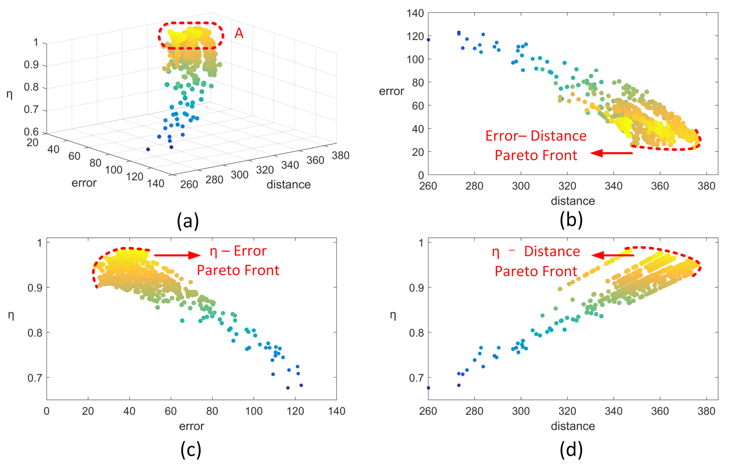
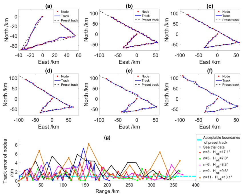
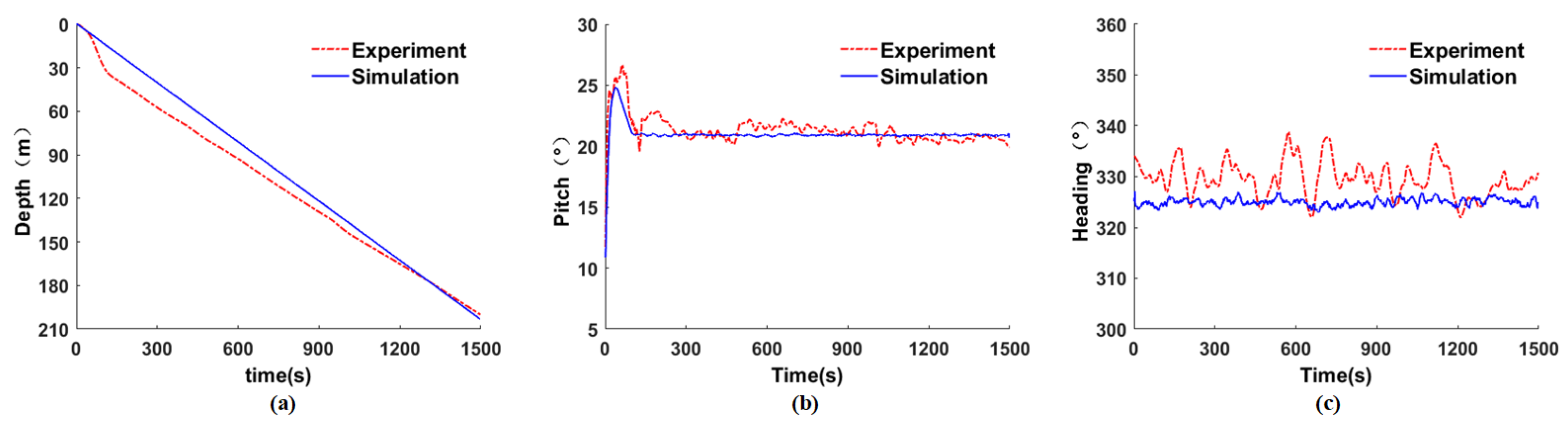
5. Numerical Simulation Results and Experiments Discussion

Using the parameters in

Table 2. Simulation parameters.

Depth	Depth	Pitch	${\mathit{H}}_{\mathit{disturb}}$	Colony Size	Maximum Iteration	Trail
500 m	450 m	23 deg	[5 deg, 10 deg]	1000	100	30

for simulation, an approximate Pareto front is obtained as a feasible solution set. Then, the final practical solution was selected through artificially participating. The objective values of the final iteration and the Pareto front are shown in Figure 9. Subplot Figure 9a is the objective function of the solution, which is the three-dimensional scatter of navigational range, heading error, and efficiency. The boxed section A represents the Pareto frontier, for which corresponding objective function has the farthest range and the smallest heading error and the highest navigation efficiency in the meantime. Figure 9b–d are projections of Figure 9a in the three orthogonal planes, respectively. The dominance of each part of the solution can be observed more intuitively through three subplots. For example, as Figure 9c shows, the red dotted line sketches out the Pareto front, compared with other objective functions of the solutions; the set members of Pareto front have a higher navigation efficiency and smaller heading error. At the same time, it can be seen that the distribution of solution points near the front of the Pareto is extensive enough, indicating that the obtained optimal solution has an acceptable representative.

Part of the optimal solution and its objective function values are shown in

Table 3. Navigation index comparison between sea trial data and several typical Pareto solutions.

n	${\mathit{H}}_{\mathit{adj}}$	R	e	$\mathbf{\eta }$	Energy Remains	Promotion on Range	Decrease on Heading Error
1	manual	205.347	1.910	0.979	0.407%	0	0
3	17.146	358.233	0.578	0.969	0.491%	74.452%	69.738%
5	7.013	366.054	0.837	0.965	0.514%	78.261%	56.178%
6	8.318	371.997	1.048	0.957	0.448%	81.115%	45.130%
9	9.625	363.448	1.387	0.941	0.724%	76.992%	27.382%
11	13.083	374.882	1.281	0.936	0.378%	82.560%	32.932%

. In order to examine the quality of the optimization results, a group of real sea trial data was cited as a benchmark, which came from the August 2019 South China Sea trial of OUC-III glider, as shown in Figure 10a. The remaining subplot shows the navigational simulation results for different control parameters. It can be seen that gliding with a large profile number (e.g., n = 11) will obtain a further navigational range but poorer accuracy to the predetermining routine even if the optimal heading adjustment angle in this situation was adopted. Conversely, with a relatively small profile number, it is well fitted to the target route; however, there were obvious defects in the gliding range. Figure 10g shows the numeric comparison of navigational objectives for different motion control parameters. Due to the occasional factors of heading angle manual adjustment and experimental uncontrollable factors, the sea trial results in range and error aspects that are less than expected. However, combining with Table 3 and Figure 10, it can still draw the conclusion that a larger number of profile increases the voyage obviously, but, despite selecting the appropriate heading adjustment angle, the heading error is still difficult to converge. In addition, based on the several sets of Pareto solutions listed above, under current environment settings, when the profile number was selected as 6 and the heading adjustment angle was chosen 13.1 deg, the overall performance of navigation is the best.

The data of depth, pitch angle, and heading angle in the actual sea trial were compared with the simulation data of the system model, as shown in Figure 11. The solid line represents the simulation curve of the model, while the dashed line represents the real data of the glider. It can be seen that the model established in this paper is close to reality, which also provides a foundation for multi-objective path planning in this paper.

6. Conclusions

Motion pattern and control parameters of underwater gliders directly influence their navigational results. Specifically, when a large profile number is applied in the practical navigation, it may obviously reduce the system energy consumption, but also trigger the problem of accumulation of heading error augmenting, which makes the motion pattern optimization and control parameter trade-off significant important. In this paper, we provide the method calculating the proper number of profiles in the engineering background to extend the gliding total range, while maintaining the preciseness of controlling the heading angle. The proposed method combined with the detailed glider dynamic model can output a set of configurable dimension Pareto solutions through the multi-objective artificial bee colony algorithm, and the solution data set has extensive representation that is convenient for flexible selection according to different practical problems. Under the preset environment disturbance conditions, a profile motion number of 6, and heading adjustment angle of 8.3 degrees, will contribute to glider navigation the most comprehensive and balanced performance. Simulation results indicate that the optimized motion prolongs the navigational range by $81\%$ and cuts the heading error by $45\%$. Relevant results provide the reference for future sea trials; meanwhile, once a more accurate marine environment modeling is used in the future work, this method can also be quickly adapted to the corresponding path planning.

References

1. Rudnick, D.L. Ocean research enabled by underwater gliders. Annu. Rev. Mar. Sci. 2016, 8, 519–541. [Google Scholar] [CrossRef] [PubMed]
2. Todd, R.E.; Rudnick, D.L.; Sherman, J.T.; Owens, W.B.; George, L. Absolute velocity estimates from autonomous underwater gliders equipped with Doppler current profilers. J. Atmos. Ocean. Technol. 2017, 34, 309–333. [Google Scholar] [CrossRef]
3. Wagawa, T.; Kawaguchi, Y.; Igeta, Y.; Honda, N.; Okunishi, T.; Yabe, I. Observations of oceanic fronts and water-mass properties in the central Japan Sea: Repeated surveys from an underwater glider. J. Mar. Syst. 2020, 201, 103242. [Google Scholar] [CrossRef]
4. Claus, B.; Bachmayer, R. Energy optimal depth control for long range underwater vehicles with applications to a hybrid underwater glider. Auton. Robot. 2016, 40, 1307–1320. [Google Scholar] [CrossRef]
5. Inanc, T.; Shadden, S.C.; Marsden, J.E. Optimal trajectory generation in ocean flows. In Proceedings of the 2005, American Control Conference, Portland, OR, USA, 8–10 June 2005; pp. 674–679. [Google Scholar]
6. Zamuda, A.; Sosa, J.D.H. Differential evolution and underwater glider path planning applied to the short-term opportunistic sampling of dynamic mesoscale ocean structures. Appl. Soft Comput. 2014, 24, 95–108. [Google Scholar] [CrossRef]
7. Song, Y.; Wang, Y.; Yang, S.; Wang, S.; Yang, M. Sensitivity analysis and parameter optimization of energy consumption for underwater gliders. Energy 2020, 191, 116506. [Google Scholar] [CrossRef]
8. Zhou, Y.; Yu, J.; Wang, X. Path planning method of underwater glider based on energy consumption model in current environment. In Lecture Notes in Computer Science, Proceedings of the International Conference on Intelligent Robotics and Applications, Guangzhou, China, 17–20 December 2014; Springer: Cham, Switzerland, 2014; pp. 142–152. [Google Scholar]
9. Fernández-Perdomo, E.; Hernández-Sosa, D.; Isern-González, J.; Cabrera-Gámez, J.; Dominguez-Brito, A.C.; Prieto-Marañón, V. Single and multiple glider path planning using an optimization-based approach. In Proceedings of the OCEANS 2011 IEEE-Spain, Santander, Spain, 6–9 June 2011; pp. 1–10. [Google Scholar]
10. Karaboga, D.; Basturk, B. A powerful and efficient algorithm for numerical function optimization: Artificial bee colony (ABC) algorithm. J. Glob. Optim. 2007, 39, 459–471. [Google Scholar] [CrossRef]
11. Akbari, R.; Hedayatzadeh, R.; Ziarati, K.; Hassanizadeh, B. A multi-objective artificial bee colony algorithm. Swarm Evol. Comput. 2012, 2, 39–52. [Google Scholar] [CrossRef]
12. Kishor, A.; Singh, P.K.; Prakash, J. NSABC: Non-dominated sorting based multi-objective artificial bee colony algorithm and its application in data clustering. Neurocomputing 2016, 216, 514–533. [Google Scholar] [CrossRef]
13. Deb, K.; Agrawal, S.; Pratap, A.; Meyarivan, T. A fast elitist non-dominated sorting genetic algorithm for multi-objective optimization: NSGA-II. In Lecture Notes in Computer Science, Proceedings of the International Conference on Parallel Problem Solving from Nature, Paris, France, 18–20 September 2000; Springer: Cham, Switzerland, 2000; pp. 849–858. [Google Scholar]
14. Li, J.Q.; Han, Y.Q. A hybrid multi-objective artificial bee colony algorithm for flexible task scheduling problems in cloud computing system. Clust. Comput. 2020, 23, 2483–2499. [Google Scholar] [CrossRef]
15. Mahmoodabadi, M.J.; Shahangian, M.M. A new multi-objective artificial bee colony algorithm for optimal adaptive robust controller design. IETE J. Res. 2019, 1–14. [Google Scholar] [CrossRef]
16. Gonzalez-Sanchez, B.; Vega-Rodríguez, M.A.; Santander-Jiménez, S.; Granado-Criado, J.M. Multi-Objective Artificial Bee Colony for designing multiple genes encoding the same protein. Appl. Soft Comput. 2019, 74, 90–98. [Google Scholar] [CrossRef]
17. Seghir, F.; Khababa, A.; Semchedine, F. An interval-based multi-objective artificial bee colony algorithm for solving the web service composition under uncertain QoS. J. Supercomput. 2019, 75, 5622–5666. [Google Scholar] [CrossRef]
18. Wang, S.X.; Sun, X.J.; Wang, Y.H.; Wu, J.G.; Wang, X.M. Dynamic modeling and motion simulation for a winged hybrid-driven underwater glider. China Ocean Eng. 2011, 25, 97–112. [Google Scholar] [CrossRef]
19. Yu, P.; Zhao, Y.; Wang, T.; Zhou, H.; Su, S.; Zhen, C. Steady-state spiral motion simulation and turning speed analysis of an underwater glider. In Proceedings of the 2017 4th International Conference on Information, Cybernetics and Computational Social Systems (ICCSS), Dalian, China, 24–26 July 2017; pp. 372–377. [Google Scholar]
Figure 1. Underwater glider system diagram.
Jmse 09 00327 g001
Figure 2. Coordinates of underwater glider.
Jmse 09 00327 g002
Figure 3. Meshing of (a) steady-state mode and (b) spiral gliding mode; (c,d) are the meshing qualities of (a,b).
Jmse 09 00327 g003
Figure 4. Dynamic pressure of direct gliding and rotating of the glider.
Jmse 09 00327 g004
Figure 5. Gliding patterns of single profile and multi-profile diagram.
Jmse 09 00327 g005
Figure 6. Diagram of glider heading adjustment in the horizontal plane: (a) the axis of the fuselage deviates from the speed; (b) Heading adjustment.
Jmse 09 00327 g006
Figure 7. Mechanism of the artificial bee colony algorithm.
Jmse 09 00327 g007
Figure 8. Flowchart of multi-objective artificial bee colony algorithm.
Jmse 09 00327 g008
Figure 9. Pareto Front and the convergence process of algorithm: (a) 3D simulation diagram of the convergence process; (bd) the projection of 3D simulation diagram on three planes.
Jmse 09 00327 g009
Figure 10. Comparison of navigation trajectories and related performances under different parameters: (a) sea trial trajectory; (bf) simulations of sailing trajectories under different parameters in Table 3; (g) the numeric comparison of trajectories for different parameters.
Jmse 09 00327 g010
Figure 11. Comparison of experimental results and simulation results: (a) depth; (b) pitch; (c) heading.
Jmse 09 00327 g011