North Sea Infragravity Wave Observations

Abstract

Coastal safety assessments with wave-resolving storm impact models require a proper offshore description for the incoming infragravity (IG) waves. This boundary condition is generally obtained by assuming a local equilibrium between the directionally-spread incident sea-swell wave forcing and the bound IG waves. The contribution of the free incident IG waves is thus ignored. Here, in-situ observations of IG waves with wave periods between 100 s and 200 s at three measurement stations in the North Sea in water depths of $O\left(30\right)$ m are analyzed to explore the potential contribution of the free and bound IG waves to the total IG wave height for the period from 2010 to 2018. The bound IG wave height is computed with the equilibrium theory of Hasselmann using the measured frequency-directional sea-swell spectra as input. The largest IG waves are observed in the open sea with a maximum significant IG wave height of $O\left(0.3\right)$ m at 32 m water depth during storm Xaver (December 2013) with a concurrent significant sea-swell wave height in excess of 9 m. Along the northern part of the Dutch coast, this maximum has reduced to $O\left(0.2\right)$ m at a water depth of 28 m with a significant sea-swell wave height of 7 m and to $O\left(0.1\right)$ m at the most southern location at a water depth of 34 m with a significant sea-swell wave height of 5 m. These appreciable IG wave heights in $O\left(30\right)$ m water depth represent a lower bound for the expected maximum IG wave heights given the fact that in the present analysis only a fraction of the full IG frequency range is considered. Comparisons with the predicted bound IG waves show that these can contribute substantially to the observed total IG wave height during storm conditions. The ratio between the predicted bound- and observed total IG variance ranges from 10% to 100% depending on the location of the observations and the timing during the storm. The ratio is typically high at the peak of the storm and is lower at both the onset and waning of the storm. There is significant spatial variability in this ratio between the stations. It is shown that differences in the directional spreading can play a significant role in this. Furthermore, the observed variability along the Dutch coast, with a substantially decreased contribution of the bound IG waves in the south compared to the northern part of the Dutch coast, are shown to be partly related to changes in the mean sea-swell wave period. For the southern part of the Dutch coast this corresponds to an increased difference with the typically assumed equilibrium boundary condition although it is not clear how much of the free IG-energy is onshore directed barring more sophisticated observations and/or modeling.

1. Introduction

The interference of sea-swell waves is controlled by the frequency-directional spectrum of the incident waves resulting in wave groups with periods between approximately 25 s to 200 s. These wave groups create a modulation in the radiation stress, forcing infragravity (IG) waves that propagate with the wave groups [1,2]. As the sea-swell wave groups approach the beach individual short waves become gradually steeper and ultimately break and dissipate their energy in the surfzone coined surfbeat by Munk [3]. The accompanying IG waves get subsequently released and (partially) reflect at the shoreline. On mildly sloping beaches this results in a dominance of IG wave energy at the waterline [4], controlling the run-up and potential overtopping at the beach [5], as well as dune erosion [6].

Modeling the impact of incident IG waves on beaches and dikes requires an offshore boundary condition that represents the incident IG waves, i.e., directed toward the coast [7]. This boundary condition is generally obtained by assuming a local equilibrium between the directionally-spread incident sea-swell wave forcing and the bound IG waves [1,8]. There are two potential problems with this approach. First, both modeling and observations have shown that the local equilibrium approach at times may significantly overestimate the sea-swell forced IG waves [9,10]. This is related to the fact that the transfer of energy from the sea-swell waves to the underlying IG waves on a sloping bed needs time and thus distance to occur. In case the changes in water depth and accompanying sea-swell conditions are large within an IG wave length, the equilibrium condition is not reached. Secondly, by using the local equilibrium it is implicitly assumed that only bound IG waves are incident on the coast. However, Ardhuin et al. [11] and Rawat et al. [12] have shown that IG waves generated at one coast can reflect and propagate across regional and even oceanic scales where they arrive as free incident IG waves at another coast. This implies that the local equilibrium approximation may in fact underestimate the incident IG energy. This contribution of the free incident IG waves to the total incident IG spectrum will depend, among other things, on the coastal configuration, where steep bathymetric slopes can trap a large part of the reflected IG energy [13]. However, in regional seas like the North Sea where the bathymetric changes are mild, a significant part of the reflected IG energy may potentially travel from coast to coast affecting the local incident IG conditions and subsequent runup and associated coastal safety during severe storms. Hence, depending on the coastal configuration, the local equilibrium approximation may result in an overestimation or underestimation of the incident IG waves.

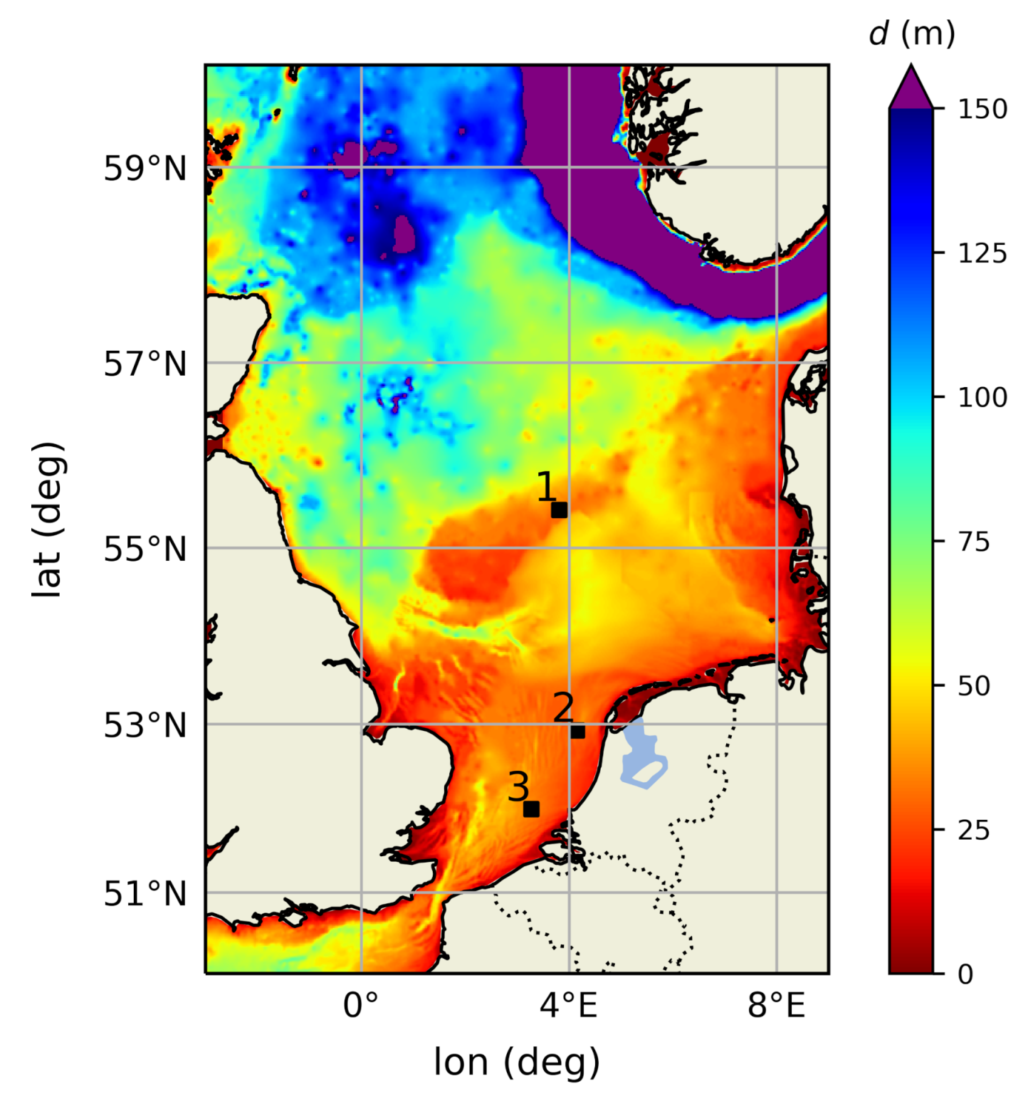
The overarching question is therefore whether the incident offshore IG conditions can be predicted with confidence using the observed local frequency-directional spectrum to predict the bound IG waves or that the free IG waves need to be taken into account to properly represent the incident IG waves in deeper water. The first step in this is to establish the role of free and bound IG waves during storm conditions. To that end, we explore the combined observations of IG waves and concurrent sea-swell conditions at the North Sea during the time period from 2010 to 2018. Observed IG wave periods are limited to a range between 100 s to 200 s due to experimental limitations and as such cover a subset of the full IG frequency spectrum. The data are analyzed to explore which part of the IG wave height can be contributed to bound IG waves during storm conditions at three measurement stations with similar depths but different coastal proximity to provide insight in their temporal evolution and spatial distribution. This is achieved by examining some of the more extreme storms in detail during this period combined with a statistical analysis of the decadal IG wave conditions. This is followed up with a discussion and recommendations for more comprehensive observations and modeling and conclusions.

2. Methods

Observations

A number of stations located in the North Sea (Figure 1) consisting of platforms equipped with instruments have been used by Rijkswaterstaat (Directorate-General for Public Works and Water Management) to collect both sea-swell and long wave data over the past nine years [2010–2018]. These observations consist of surface elevation spectra covering both sea and swell conditions, with frequencies $0.04<f<0.5$ Hz, and low-pass filtered surface elevation time series with $f<0.025$ Hz in continuous blocks of 10 min [14]. Taking the average of six consecutive 10-min sea-swell spectra and concatenating the six corresponding blocks of low-pass filtered surface elevation, hourly records have been created for further analysis. The first station, A12 (see

Table 1. Station and instrument information. Radar: Saab L2. Step gauge: Marine 300. Wave buoy: Datawell.

Name	No.	Lat	Long	Depth (m)	Water Level Inst.	Directional Inst.
A12	1	55.417	3.817	32.6	Radar	Wave buoy
Q1	2	52.925	4.150	28.2	Step Gauge	Wave buoy
EUR	3	51.998	3.275	34.8	Radar	Wave buoy

), is located in the center of the southern North Sea whereas the other two stations are in close proximity of the Dutch coast (see Figure 1), all at similar depths of $O\left(30\right)$ m. Both the sea-swell frequency spectra and the low-pass filtered IG time series are based on the surface elevation measured with either a step-gauge or radar with a sampling frequency of 2.56 Hz. The finite vertical resolution of 2 cm for the step gauge and 1 cm for the radar introduces a step-wise change in the observed surface elevation. Previous research suggests that this does not significantly affect the results at the IG frequencies provided that the standard deviation of the surface elevation is larger than half the vertical resolution [15]. The directional distribution of the sea-swell waves has been obtained with a directional wave buoy. Station coordinates, local depth and instrumentation are given in Table 1.

The significant wave height of the sea-swell waves is given by:

$$H_{m0,ss}=4\sqrt{{\int }_{f=0.04\mathrm{Hz}}^{f=0.5\mathrm{Hz}}{E}_{ss}\left(f\right)df}=4\sqrt{m0}$$

(1)

with $E_{ss}$ representing the hourly surface elevation variance density of the sea-swell waves obtained by averaging over six 10 min blocks. The corresponding mean sea-swell period is obtained from:

$$T_{m0,-2,ss}=\sqrt{\frac{{\int }_{0.04\mathrm{Hz}}^{0.5\mathrm{Hz}}{f}^{-2}{E}_{ss}\left(f\right)df}{m0}}$$

(2)

The frequency-dependent primary wave direction, ${\theta }_p\left(f\right)$ and directional spreading, ${\sigma }_{\theta }\left(f\right)$, obtained at the three stations equipped with a directional wave buoy are used to construct the hourly frequency-directional spectra, $E_{ss}(f,\theta )$:

$$E_{ss}(f,\theta )=E_{ss}\left(f\right)D(\theta ,f)$$

(3)

where $D(\theta ,f)$ is the frequency-dependent directional distribution function (see Appendix A). The mean sea-swell wave direction is obtained from:

$${\theta }_{ss}={tan}^{-1}\left[\frac{{\int }_{0.04\mathrm{Hz}}^{0.5\mathrm{Hz}}sin\left({\theta }_p\left(f\right)\right)E_{ss}\left(f\right)df}{{\int }_{0.04\mathrm{Hz}}^{0.5Hz}cos\left({\theta }_p\left(f\right)\right)E_{ss}\left(f\right)df}\right]$$

(4)

and the mean sea-swell directional spreading is given by:

$${\sigma }_{\theta ,ss}=\frac{{\int }_{0.04\mathrm{Hz}}^{0.5\mathrm{Hz}}{\sigma }_{\theta }\left(f\right)E_{ss}\left(f\right)df}{m0}$$

(5)

The long wave surface elevation was obtained by applying a low-pass FIR filter to the original surface elevation time series sampled at 2.56 Hz (see Appendix B) and sub-sampled at a 12.5 s interval. This was done to limit the data transfer from the platforms to shore where the data was collected. IG spectra ($E_{ig}$) are calculated from one-hour records of these low-pass surface elevation data with a resolution of 0.0025 Hz and 48 degrees of freedom. To compensate for the minor amplitude attenuation for frequencies up to 0.01 Hz, an inverse filter has been applied to obtain the true IG wave spectra (see Appendix B). At higher IG frequencies, the attenuation increases rapidly making this approach susceptible to noise resulting in potentially erroneous estimates of the IG variance density. These higher IG frequencies (0.01–0.04 Hz) are thus excluded from further analysis and the IG wave height is obtained from:

$$H_{m0,ig,t}=4\sqrt{{\int }_{f=0.005\mathrm{Hz}}^{f=0.01\mathrm{Hz}}{E}_{ig}\left(f\right)R^{-2}\left(f\right)df}$$

(6)

where $E_{ig}$ represents the variance density spectrum of the low-pass filtered time series and R is the filter-induced amplitude attenuation factor (see Appendix B).

The frequency-directional sea-swell spectra are used to predict the bound IG wave spectrum with the equilibrium theory derived by Hasselmann [8] using the near-bed pressure formulation of Herbers et al. [16] (see Appendix C). To that end, the frequency-directional sea-swell spectra, $E_{ss}(f,\theta )$, have been translated to directional near-bed pressure spectra using linear wave theory taking into account changes in the local water depth due to the tide and storm surge. The estimated bound IG wave height is obtained from:

$$H_{m0,ig,b}=4\sqrt{{\int }_{f=0.005\mathrm{Hz}}^{f=0.01\mathrm{Hz}}{E}_b\left(f\right)df}$$

(7)

where $E_b$ is the variance density of the predicted bound IG spectrum. The difference between the observed total IG wave height and the predicted bound IG wave height is attributed to free IG waves and is obtained by subtracting the bound part from the total IG wave height according to:

$$H_{m0,ig,f}=\sqrt{H_{m0,ig,t}^2-H_{m0,ig,b}^2}$$

(8)

The squared ratio of the bound IG wave height over the total IG wave height:

$$R_{ig,b}^2={\left(\frac{H_{m0,ig,b}}{H_{m0,ig,t}}\right)}^2$$

(9)

is used to examine the relative contribution of the bound IG variance to the total IG variance.

3. Results

3.1. IG Wave Climate

In the following, the period from 2010–2018 is used to examine the IG wave climate. Only cases where the observed directional spreading was available to reconstruct the sea-swell frequency-directional spectrum (Appendix A) are considered as this is a prerequisite to predict the bound portion of the IG field. The IG response to storm conditions with $H_{m0,ss}>3$ m at A12 exhibits high IG variance at times of large sea-swell wave heights (panel A of Figure 2). The highest IG wave heights occur for sea-swell waves incident from the north–west, $-{90}^{\circ }<\theta <0^{\circ }$, ($H_{m0,ig,t}\approx 0.3$ m, see black dots in panel B of Figure 2) corresponding to the longest fetch (see Figure 1).

The predicted bound IG variance at A12 gives a lower bound for the total IG variance (see upper panels of Figure 2). The relative difference with the bound IG variance is largest for the milder sea-swell storm conditions consistent with a predominance of free IG waves. Furthermore, this predominance is directionally dependent with relatively more bound IG variance for sea-swell waves incident from the south to south–east, ${90}^{\circ }<\theta <{150}^{\circ }$ corresponding to the red colors in panel B of Figure 2, and significantly more free IG variance for sea-swell waves incident from the south–west to west with $-{150}^{\circ }<\theta <-{90}^{\circ }$ (corresponding to the blue colors in panel B of Figure 2). During extreme sea-swell conditions, the relative difference with the predicted bound variance decreases but is at times still substantial with a clear dominance of free IG waves at this location. The fact that the observed total IG variance has a common cut-off around ${10}^{-3}$ m${}^2$ suggests that there is a background IG signal or instrument noise with a significant wave height of $O\left(3\right)$ cm.

The IG wave response for the same storm conditions at station Q1, located along the northern part of the Dutch coast at a depth of 28.2 m (see Figure 1) shows a similar pattern with the predicted bound IG variance acting again as a lower bound (see panel C of Figure 2). The spreading of the total IG variance for a given sea-swell wave height is notably smaller compared with station A12. In addition, the IG variance has been reduced compared to station A12, whereas the apparent IG noise level has been maintained. A further reduction in IG variance is observed at station EUR (see panel D of Figure 2). This station is located along the southern part of the Dutch coast at a depth of 34 m (see Figure 1). Here the IG wave conditions are at all times dominated by free IG waves as is evident from the large relative difference with the predicted bound IG variance. To understand the observed differences in IG response at the three locations two major storms, Xaver and Egon, are examined in more detail next.

3.2. Xaver

The storm Xaver is the most severe in terms of $H_{m0,ss}$ within the total data set resulting in a strong IG response (see magenta circles in Figure 2). Xaver occurred at the beginning of December 2013 with sea-swell wave heights in excess of 9 m at location A12 during the peak of the storm around midnight on the 5th of December (panel A in Figure 3). The wave height at location Q1 is significantly reduced compared with A12 with a maximum close to 7 m, which is reached approximately three hours after the peak of the storm at A12. A further reduction is observed at the most southerly station EUR with a maximum wave height of $O\left(5\right)$ m that is reached around noon on 5 December. The evolution of the sea-swell wave direction is similar at all three locations showing a gradual change from north–west to north with a slight delay in time for stations Q1 and EUR (panel B in Figure 3). With the change in direction the wave period increases at stations A12 and Q1 with maxima in the order of 14 and 12 s, respectively. The sea-swell wave period at EUR stays around 10 s for the duration of the storm (panel C in Figure 3). The mean directional spreading at A12 is significantly larger than the spreading at the other stations (see panel D in Figure 3 and directional spectra in Appendix A).

Computing the observed IG wave height with Equation (6) shows that at times of moderate sea-swell wave conditions prior to the storm a background IG signal is present with a wave height in the order of a few centimeters at all three locations (see panels A to C in Figure 4). The measured IG wave height at A12 has three local maxima at T = 5.6, 6 and 6.5 days, respectively, that coincide with the maxima in the sea-swell wave height (compare with panel A in Figure 3). During the peak of the storm around midnight of 5 December the IG wave height reaches $O\left(0.30\right)$ m. A similar pattern in the IG wave height is observed at station Q1, although it has been reduced in height and delayed in time by approximately 3 h compared to station A12. The maximum IG wave height of $O\left(0.2\right)$ m is subsequently reached around 3 a.m. on 6 December. The IG wave height at EUR is reduced even further compared to Q1 with a local maximum in the order of 0.1 m around 4 a.m. on 6 December.

Computing the bound IG wave height with Equation (8) based on the hourly frequency-directional spectra (Appendix A), shows that the observed IG wave height at A12 is at all times larger than the predicted bound IG wave height during the storm (see panel A in Figure 4). The ratio of bound IG variance over the total IG variance stays around 0.25 for the duration of the storm (see panel D in Figure 4). This is different for the first part of the storm at station Q1, where the bound IG variance contribution peaks at $O\left(60\right)\%$ of the total IG variance (see panels B and D in Figure 4). After that, the ratio at Q1 gradually drops again indicative of an increased relative contribution of free IG waves. At station EUR, the predicted bound IG height is only a fraction of the observed IG height, with a peak at the onset of the storm around noon of Dec 5 where it contributes a maximum of $O\left(10\right)$% to the total IG variance corresponding to an IG sea state that is at all times dominated by free IG waves.

3.3. Egon

The storm Egon occurred on the 13th of January 2017 with a rapid increase in the sea-swell wave height to a maximum of 8.5 m at station A12 (see upper panel of Figure 5). The peak sea-swell wave heights at Q1 and EUR are again reduced compared to A12 and occurred about 3 to 4 h later. During the storm, the mean direction was more or less constant from the NNW at all three locations (see panel B in Figure 5). The sea-swell wave periods at A12 shows the largest increase compared with the onset of the storm reaching a value of 13 s. Maximum sea-swell wave periods at Q1 and EUR are 12 and 9.5 s, respectively. The directional spreading at station A12 is very narrow at the onset of the storm with a value of ${20}^{\circ }$ and stays below ${30}^{\circ }$ for the duration of the storm. The directional spreading at the other stations is wider with a mean value of $O\left({40}^{\circ }\right)$ and a minimum of ${30}^{\circ }$ (see panel D in Figure 5), similar to what was observed during Xaver.

The IG response is the strongest at station A12 with a maximum IG wave height of $O\left(0.25\right)$ m at the peak of the storm (Figure 6). The maximum IG wave height at Q1 is smaller, $O\left(0.15\right)$ m, and occurs a short time after the maximum sea-swell wave height has passed at Q1 (compare panels A and B in Figure 5 and Figure 6, respectively). The IG wave height at station EUR is $O\left(0.1\right)$ m with a temporal distribution similar to station Q1. The predicted bound IG wave height at A12 lags behind the total IG height at the onset of the storm, but is close to the total IG height at the peak of the storm (see panel A and D in Figure 6 around T = 13.75 days). At Q1 the maximum contribution of the bound IG variance briefly reaches $O\left(60\right)$% a couple of hours before midnight on 13 January. Thereafter, it quickly drops to $O\left(30\right)$% around T = 14 days as the total IG wave height remains high while at the same time the bound IG wave height decreases (see panels B and D in Figure 6). At EUR the maximum bound IG variance contribution is again less than 10% of the total IG variance at all times.

3.4. Storm-Averaged Temporal Response

The IG response depends on the local sea-swell conditions as is evident from Xaver and Egon. Averaging both sea-swell heights and IG heights for a number of similar storms with less than 15% variation in both sea-swell wave height and wave period at the peak of the storm at a given location (see

Table 2. Named storms included (x) or excluded due to data unavailability (o) in estimating the storm-averaged temporal IG response at the three stations. Mean sea-swell wave direction at the peak of the storm at A12 is given by ${\theta }_{ss,p}$ using the nautical convention.

Name	Date	A12	Q1	EUR	${\mathit{\theta }}_{\mathbf{ss},\mathit{p}}{(}^{\circ })$
Friedhelm	8–10 December 2011	x	x	x	−65
Xaver	5–8 December 2013	x	x	x	−38
Egon	13–15 January 2017	x	x	x	−26
Axel	3–5 January 2017	x	x	x	−20
Christian	27–28 October 2013	o	x	x	−125

) gives insight in the storm-averaged temporal response at the different stations.

To enable the averaging, a common time axis has been defined centered at the peak of the sea-swell wave heights. At A12, the maximum in the total IG wave height occurs at the peak of the storm coinciding with the maximum in the bound IG wave height (compare panels A and B in Figure 7). At this time, the free IG wave height is close to the bound IG height, each contributing 50% to the total IG variance. Note that the peak in the free IG wave height is reached a few hours before the peak of the storm. The growth rate in IG wave height for the free and bound components is comparable prior to the peak of the storm. However, after the peak has passed, the decay rate of the bound IG wave height is significantly larger than that of the free IG wave height resulting in a clear dominance of free IG waves (see panel B in Figure 7). At Q1 the IG response is more symmetric centered around the peak in sea-swell wave height (see panels C and D in Figure 7). Here, the maximum IG response for both the free and bound components occurs at the peak of the storm, again with an equal contribution of 50% to the total IG variance. Both prior and after the peak of the storm, IG wave conditions are dominated by free IG waves. At EUR, the bound and free IG wave height response is also symmetrically centered around the peak of the storm (see panels E and F in Figure 7), however the contribution of the bound IG wave height to the total IG height is very small consistent with a predominance of free IG waves at all times.

3.5. IG Wave Statistics

The IG wave height as a function of the sea-swell wave height during all storm conditions is considered next. To that end, the sea-swell wave heights have been collected in 1 m wide bins. This shows a clear non-linear increase in the total median IG wave height at A12 with increasing $H_{m0,ss}$ (see Panel A in Figure 8). The corresponding bound IG wave height shows a slightly stronger increase (panel B) and as a result only a slow decrease in the median contribution of the free IG waves to the total IG variance (see Panel C in Figure 8) consistent with the persistent predominance of free IG waves. Q1 also exhibits a non-linear increase in the total IG wave height as function of the sea-swell forcing (see Panel D in Figure 8). This is accompanied with a relatively stronger non-linear increase in the bound IG wave height (panel E) resulting in a significant non-linear decrease in the contribution of the free IG waves to the total variance (see Panel F in Figure 8) reaching a minimum median value of $O\left(40\right)$%. At station EUR, the IG-wave height increases more or less linearly with the sea-swell forcing (see Panel G in Figure 8) as does the bound IG wave height (panel H). This results in a clear dominance of the free IG waves (see Panel I in Figure 8). Note that the IG response for sea-swell waves higher than 6 m is missing as these did not occur at EUR in the 2010–2018 time frame.

4. Discussion

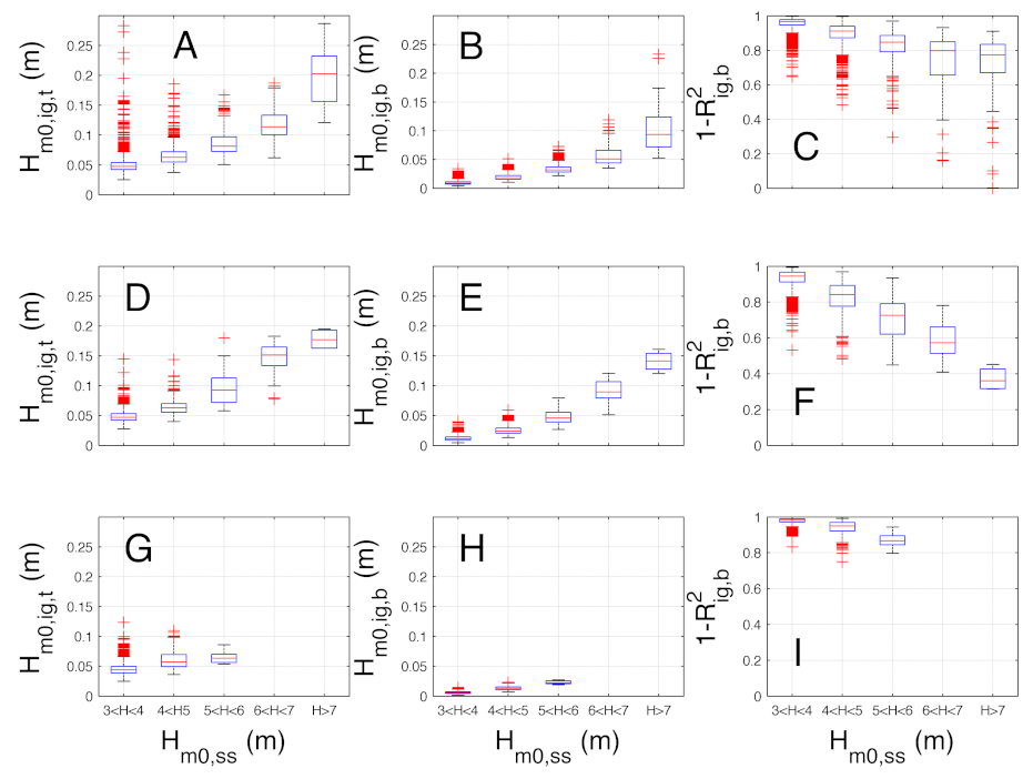
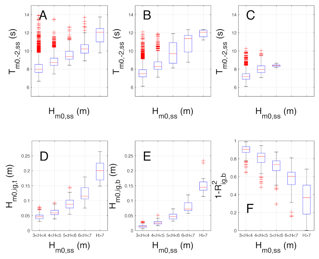
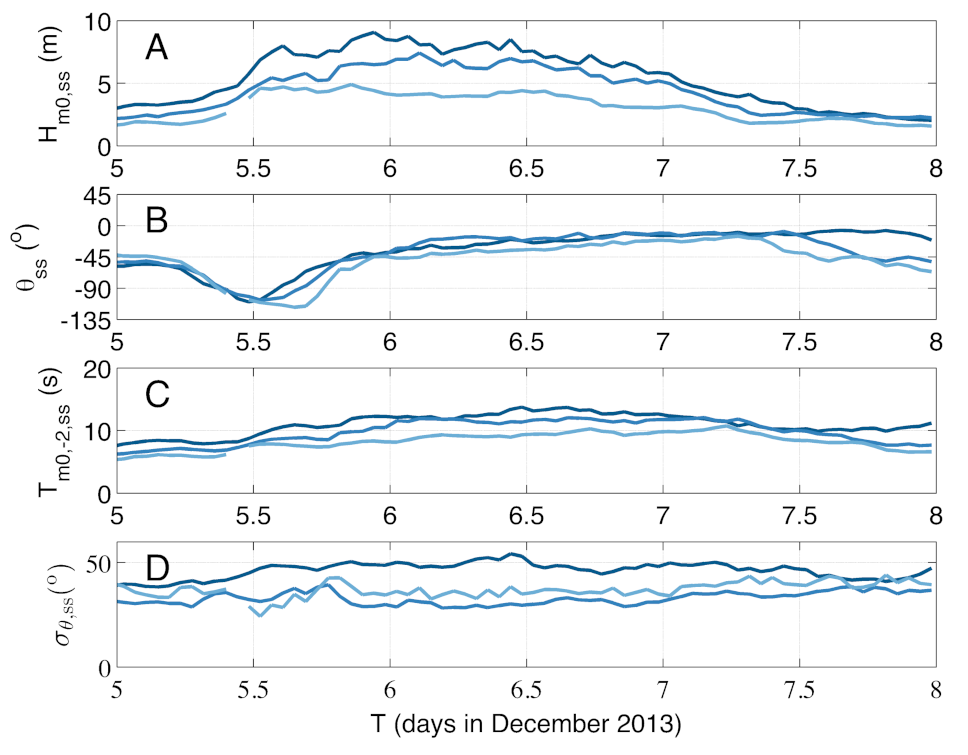
The observations show that there are significant differences in the observed total IG wave height at the different stations that cannot be explained by the differences in IG wave shoaling associated with small differences in local water depth (see Table 1). Part of the spatial variability can be attributed to changes in the bound IG wave height response (compare panels B, E and H in Figure 8). For the lower sea-swell wave conditions the predicted bound IG wave heights at EUR are typically smaller than at the other stations. As a result, they contribute only marginally to the total IG wave height that is similar at all stations for these moderate sea-swell wave heights. This lower IG response is consistent with the fact that the median mean sea-swell wave period at EUR is shorter than at the other stations (compare panels C with A and B in Figure 9) and somewhat larger water depth (see Table 1) resulting in a smaller interaction coefficient (see Appendix C). For the higher sea-swell wave heights the bound IG wave height is largest at Q1. This in turn can be attributed to the larger median mean sea-swell period (compare panels B with A in Figure 9) as well as the slightly smaller water depth at this location. 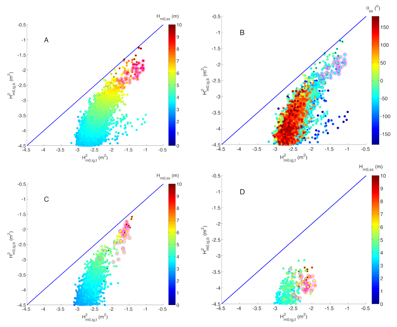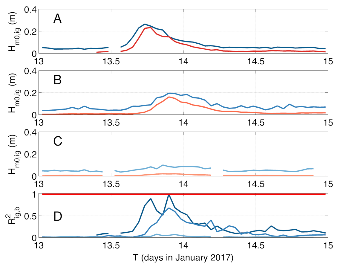As the median mean wave period for the bin with the highest sea-swell waves is similar at Q1 and A12, it does not explain why the median bound IG wave height is significantly larger at Q1 (compare panels B and E in Figure 8). Furthermore, for the higher sea-swell wave heights, IG wave statistics at A12 show a persistent predominance of free IG waves that is in contrast with the observations during Egon with an approximately 100 % contribution by bound IG waves at the peak of the storm (compare panels A and D in Figure 6 and panel C in Figure 8). This apparent mismatch can be explained by the differences in directional spreading of the sea-swell waves where a narrow spreading is expected to lead to an increased contribution of the bound IG wave (see Appendix C) and subsequent decreased contribution of the free IG waves [16]. Restricting the IG cases to sea-swell cases with a directional spreading of less or equal than 30${}^{\circ }$ confirms this where the median bound IG wave height at A12 has increased substantially (compare panels D, E and F with A, B and C in Figure 8 and Figure 9, respectively) whereas the results at Q1 are not affected (not shown).

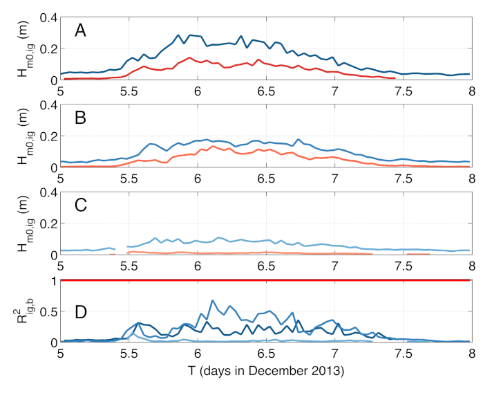
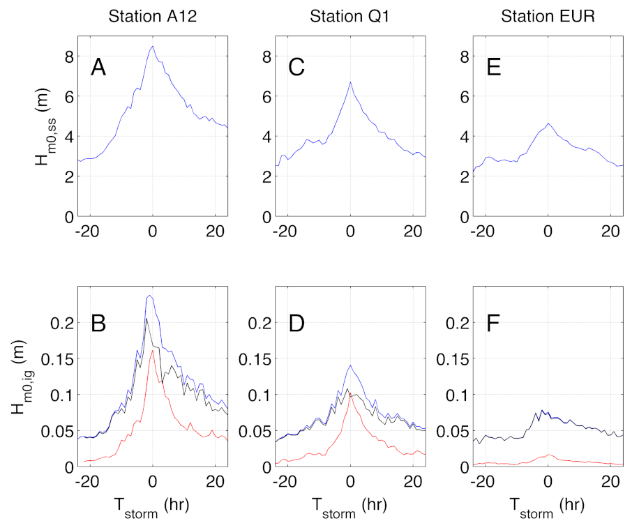
Spatial variability in the total IG wave height will also result from changes in the free IG waves related to refraction, reflection and trapping, dissipation by bed friction and differences in the non-linear transfer and release from the sea-swell waves forcing the IG waves. This is for instance evident in the storm-averaged temporal response (see Figure 7) exhibiting a significant increase in the total IG wave signal at the onset of the storm that is different at the three locations. The majority of this increase is related to free IG waves that are preceding the peak of the storm. Based on the observations, it is not clear whether these IG forerunners are related to the earlier release of bound IG waves due to bathymetric variability (see Figure 1), the generation by other mechanisms like wind gusts [17] or the arrival of reflected IG waves from nearby up-wave coasts [11,12]. The predominance of free IG waves trailing the peak of the storm is consistent with the reflection and trapping of IG waves in the down-wave sea-swell direction.

The bound IG estimates are based on the reconstructed frequency-directional sea-swell spectra (Appendix A and Appendix C). The fact that the reconstruction only allows for uni-modal directional distributions may result in inaccurate estimations, especially at times of broad directional spreading. As the time-series of the sea-swell surface elevation are not available, this potential error in the estimated bound portion of the IG waves cannot be verified with a bi-spectral analysis [18] and hence it is not known how well the predicted bound IG wave heights correspond to the observations under these conditions.

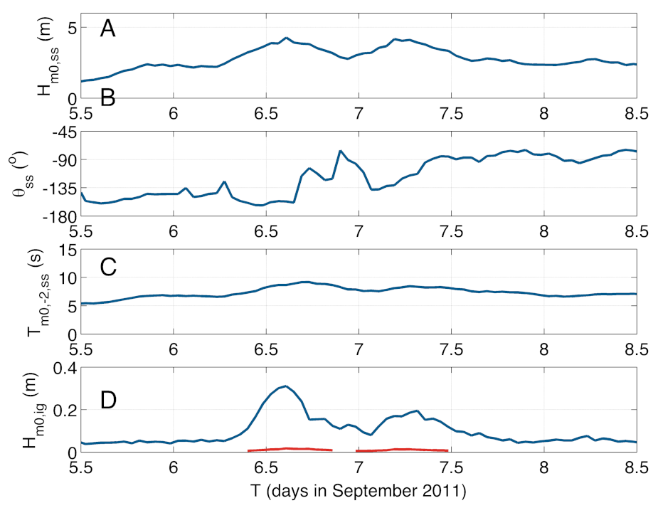
It is noted that by excluding the spectra with a broad directional spreading, the outliers for the lower sea-swell wave height bins have been removed (compare left panel of Figure 9 with panel A in Figure 8 for $H_{m0,ss}\le 5$ m). The bulk of these outliers are associated with a single event in September of 2011 and are only present at A12 (see Figure 10). At that time, the sea-swell waves are incident from the southerly direction with a moderate storm wave height of $O\left(4\right)$ m and wave period of less than 10 s. As expected, this results in a minimal contribution of the bound IG variance to the observed total IG variance (see panel D in Figure 10). There is no indication that the observations are erroneous and as such may be related to the resonant transfer from the spatially varying wind forcing or air pressure fluctuations that are known to occur within the southern part of the North Sea [19].

The offshore boundary condition for IG storm impact computations requires the incident part of the IG waves, i.e., the onshore directed components. However, the directional information on the IG energy propagation is missing as the measurements consider the surface elevation only and thus a separation of the incident and reflected IG wave components is not possible at this time. However, combining the current observations with numerical modeling can shed light on the directional properties of the IG waves as well. One promising approach is the use of a backward ray-tracing method to examine the wave rays of the free IG waves radiating away from the coast showing the potential effects of refractive trapping (e.g., [13]). Alternatively, the approach outlined by Ardhuin et al. [11] can be used to examine the refractive trapping and leakage of the reflected IG waves with a spectral wave model. In that case, a directionally isotropic IG source along the coast is imposed as a boundary condition with an intensity that is based on a parametric expression involving the incident sea-swell wave height, period and local water depth:

$${\alpha }_1{H}_{m0,ss}{T}_{m0,-2}^2\sqrt{\frac{g}{h}}$$

(10)

where g is the gravitational acceleration, h is the local water depth and ${\alpha }_1$ is a spatially dependent constant.

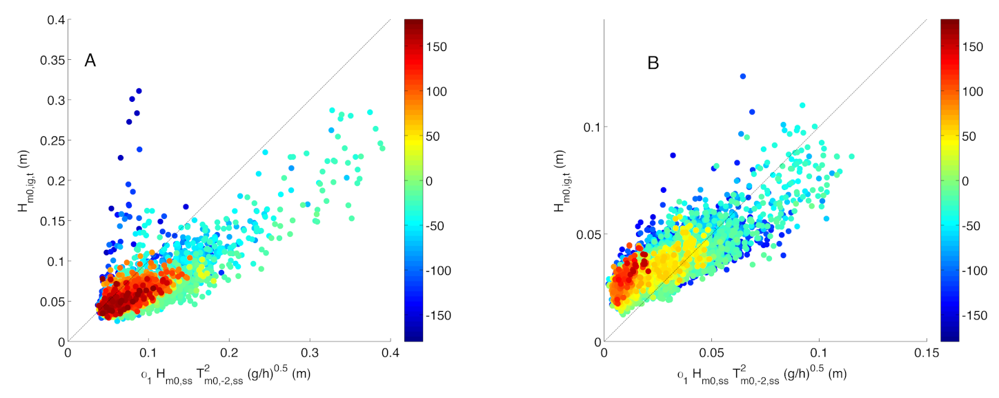
Ardhuin et al. [11] found a near linear dependence between the IG wave height and ${\alpha }_1$ at different measuring stations with a mean value of $O\left(5e^{-4}\right)$ s${}^{-1}$. Examining this relationship for the three stations shows that using a constant value for ${\alpha }_1$ is not representative for all incident sea-swell wave directions. At A12, the earlier mentioned anomalous response for sea-swell waves from the southerly directions is clearly visible (see blue dots in Panel A of Figure 11). The IG response for the other directions is more or less constant. This is different from the IG response at both Q1 (not shown) and EUR (panel B of Figure 11), where waves incident from the easterly directions create a relatively stronger response in the IG wave height compared to sea-swell waves incident from the westerly directions. This is to be expected if the beach characteristics, most notably the beach slope, are different at the coast where free IG waves are reflected from. By examining the IG response for different storms it should be possible to obtain spatially dependent estimates of the ${\alpha }_1$ scaling factor. These modeling efforts should ideally be supported with additional field observations of co-located velocity and surface elevation or pressure measurements to compare with the model predicted directional properties of the IG waves and more specifically the incident free IG component.

The IG waves discussed here have been observed in water depths between 28 m and 34 m (see Table 1) and are expected to increase substantially between these depths and the nearshore. In the case of free IG waves, this transformation is similar to the incident sea-swell waves where refraction and shoaling are important [11]. For the bound IG waves this is controlled by the non-linear interaction with the sea-swell waves, which depends strongly on the frequency-directional distribution of the latter as well as the beach slope [9,10]. The relative importance of these processes will determine the potential storm impact of the free IG waves and bound IG waves at the coast.

5. Conclusions

In-situ observations of IG waves with wave periods between 100 s and 200 s at three measurement stations in the North Sea in water depths of $O\left(30\right)$ m have been analyzed to explore the potential contribution of the bound and free IG waves to the total IG wave height for the period from 2010 to 2018. The largest IG waves are observed in the open sea with a maximum significant IG wave height of $O\left(0.3\right)$ m at 32 m water depth during storm Xaver with a concurrent significant sea-swell wave height in excess of 9 m. Along the northern part of the Dutch coast, this maximum has reduced to $O\left(0.2\right)$ m at a water depth of 28 m with a sea-swell wave height of 7 m and to $O\left(0.1\right)$ m at the most southern location at a water depth of 34 m with a significant sea-swell wave height of 5 m. Comparisons with the predicted bound IG waves show that these can contribute substantially to the observed total IG wave height during storm conditions. The ratio between the predicted bound- and observed total IG variance ranges from 10% to 100% depending on the location of the observations and the timing during the storm. The ratio is typically high at the peak of the storm and is lower at both the onset and waning of the storm. There is also significant spatial variability in this ratio between the stations. It is shown that differences in the directional spreading can play a significant role in this. Furthermore, the observed variability along the Dutch coast, with a substantially decreased contribution of the bound IG waves in the south compared to the northern part of the Dutch coast, are shown to be partly related to changes in the mean sea-swell wave period. Although this corresponds to an increased difference with the typically assumed equilibrium boundary condition, it is not clear how much of the free IG-energy is onshore directed barring more sophisticated observations and/or modeling. The total IG wave height correlates well with the local wave parameter introduced by Arhuin et al. [11], however the correlation for the two stations located at the Dutch coast is directionally dependent. This suggests that differences in the beach characteristics where the free IG waves originate from play an important role. Finally it is noted that in the present analysis only a fraction of the IG-spectrum is considered, with wave periods between 100 s and 200 s, and as such the already appreciable IG wave heights in $O\left(30\right)$ m water depth are a lower bound estimate for the full IG frequency range of 0.005–0.04 Hz.

References

1. Longuet-Higgins, M.S.; Stewart, R.W. Radiation stress and mass transport in gravity waves, with application to ‘surf beats’. J. Fluid Mech. 1962, 13, 481–504. [Google Scholar] [CrossRef]
2. Biesel, F. Equations generales au second ordre de la houle irreguliere. Houille Blanche 1952, 7, 372–376. [Google Scholar] [CrossRef] [Green Version]
3. Munk, W.H. Surf beats. Trans. Am. Geophys. Union 1949, 30, 849–854. [Google Scholar]
4. Holman, R.A. Extreme value statistics for wave run-up on a natural beach. Coast. Eng. 1986, 9, 527–544. [Google Scholar] [CrossRef]
5. Stockdon, H.F.; Holman, R.A.; Howd, P.A.; Sallenger, A.H. Empirical parameterization of setup, swash and runup. Coast. Eng. 2006, 53, 573–588. [Google Scholar] [CrossRef]
6. van Thiel de Vries, J.S.M.; van Gent, M.R.A.; Walstra, D.J.R.; Reniers, A.J.H.M. Analysis of dune erosion processes in large-scale flume experiments. Coast. Eng. 2008, 55, 1028–1040. [Google Scholar] [CrossRef]
7. Fiedler, J.W.; Smit, P.B.; Brodie, K.L.; McNinch, J.; Guza, R. The offshore boundary condition in surf zone modeling. Coast. Eng. 2019, 143, 12–20. [Google Scholar] [CrossRef]
8. Hasselmann, K. On the non-linear energy transfer in a gravity-wave spectrum Part 1. General theory. J. Fluid Mech. 1962, 12, 481–500. [Google Scholar] [CrossRef]
9. Battjes, J.A.; Bakkenes, H.J.; Janssen, T.T.; van Dongeren, A.R. Shoaling of subharmonic gravity waves. J. Geophys. Res. Ocean. 2004, 109. [Google Scholar] [CrossRef] [Green Version]
10. Herbers, T.H.C.; Burton, M.C. Nonlinear shoaling of directionally spread waves on a beach. J. Geophys. Res. 1997, 102, 21101–21114. [Google Scholar] [CrossRef]
11. Ardhuin, F.; Rawat, A.; Aucan, J. A numerical model for free infragravity waves: Definition and validation at regional and global scales. Ocean Model. 2014, 77, 20–32. [Google Scholar]
12. Rawat, A.; Ardhuin, F.; Ballu, V.; Crawford, W.; Corela, C.; Aucan, J. Infragravity waves across the oceans. Geophys. Res. Lett. 2014, 41, 7957–7963. [Google Scholar] [CrossRef] [Green Version]
13. Smit, P.B.; Janssen, T.T.; Herbers, T.H.C.; Taira, T.; Romanowicz, B.A. Infragravity wave radiation across the shelf break. J. Geophys. Res. Ocean. 2018, 123, 4483–4490. [Google Scholar] [CrossRef]
14. Kamminga, S.; Koster, T. Een Algortime Voor de Opslag van Data van Lange Golven; Ingenieursburo S.D. Kamminga B.V.: Zoetermeer, The Netherlands, 2001. [Google Scholar]
15. de Valk, C.F. Long Waves on the North Sea: An Investigation of the Requirements on Measurement and Data Processing; Deltares (WL): Delft, The Netherlands, 1992. [Google Scholar]
16. Herbers, T.; Elgar, S.; Guza, R. Infragravity-frequency (0.005–0.05 Hz) motions on the shelf. Part I: Forced waves. J. Phys. Oceanogr. 1994, 24, 917–927. [Google Scholar] [CrossRef]
17. Vrecica, T.; Soffer, R.; Toledo, Y. Infragravity wave generation by wind gusts. Geophys. Res. Lett. 2019, 46. [Google Scholar] [CrossRef]
18. Hasselmann, K.; Munk, W.; MacDonald, G. Bispectra of Ocean Waves; Time Series Analysis; Rosenblatt, M., Ed.; Wiley: Hoboken, NJ, USA, 1963; pp. 125–139. [Google Scholar]
19. de Jong, M.P.C.; Holthuijsen, L.H.; Battjes, J.A. Generation of seiches by cold fronts over the southern north sea. J. Geophys. Res. 2003, 108. [Google Scholar] [CrossRef]
Figure 1. Bathymetry of the southern part of the North Sea basin. Locations of measuring stations given by black markers and numbers (see Table 1 for more information). The color bar corresponds to water depth in m with respect to mean sea level.
Jmse 09 00141 g001
Figure 2. Hourly observations of total infragravity (IG) variance ( H m 0 , i g , t 2 ) versus predicted bound IG variance ( H m 0 , i g , b 2 ) for storm conditions ( H m 0 , s s > 3 m) at station A12 from 2010–2018. The colors in the panels (A,C,D) show the sea-swell wave height ( H m 0 , s s ) at A12, Q1 and EUR, respectively (color bar in m). The colors in panel (B) correspond to the mean sea-swell wave direction ( θ s s ) at A12 (color bar in nautical degrees, the direction where waves come from measured clockwise from geographic north). Open circles highlight conditions corresponding to the peak of storm Xaver and black dots to storm Egon, respectively. Results are presented at a log10 scale where −1 corresponds to 10 1 .
Jmse 09 00141 g002
Figure 3. Sea-swell conditions during storm Xaver at locations A12 (dark blue), Q1 (blue) and EUR (light blue). (A) Significant Wave height H m 0 , s s . (B) Mean wave direction θ s s (Nautical convention). (C) Wave period T m 0 , 2 , s s . (D) Mean directional spreading σ θ , s s .
Jmse 09 00141 g003
Figure 4. IG conditions during storm Xaver at locations A12 (dark blue), Q1 (blue) and EUR (light blue). (A) Bound (red) and total (blue) IG wave height at A12. (B) Bound (red) and total (blue) IG wave height at Q1. (C) Bound (red) and total (blue) IG wave height at EUR. (D) Ratio of the predicted bound IG variance over the observed IG variance where the red line corresponds to zero difference.
Jmse 09 00141 g004
Figure 5. Sea-swell conditions during storm Egon at locations A12 (dark blue), Q1 (blue) and EUR (light blue). (A) Significant Wave height. (B) Mean wave direction (Nautical convention). (C) Wave period T m 0 , 2 . (D) Mean directional spreading.
Jmse 09 00141 g005
Figure 6. IG conditions during storm Egon at A12 (dark blue), Q1 (blue) and EUR (light blue). (A) Bound (red) and total (blue) IG wave height at A12. (B) Bound (red) and total (blue) IG wave height at Q1. (C) Bound (red) and total (blue) IG wave height at EUR. (D) Ratio of the predicted bound IG variance over the observed IG variance where the red line corresponds to zero difference.
Jmse 09 00141 g006
Figure 7. (A,C,E) Storm averaged sea-swell wave height centered around the peak of the storm at A12, Q1 and EUR, respectively. (B,D,F) Storm-averaged IG total (blue), free (black) and bound (red) IG wave heights at A12, Q1 and EUR, respectively.
Jmse 09 00141 g007
Figure 8. (A,D,G) Box-whisker plots of the total IG wave height as a function of the binned sea-swell wave height at A12, Q1 and EUR, respectively. (B,E,H) Box-whisker plots of the bound IG wave height as a function of the binned sea-swell wave height at A12, Q1 and EUR, respectively. (C,F,I) Box-whisker plots of the contribution of the free IG waves to the total IG variance at A12, Q1 and EUR, respectively. The box includes the 25 to 75 percentiles with the median in red. Outliers are given by the red plus signs.
Jmse 09 00141 g008
Figure 9. (A) Box-whisker plot of the mean wave period as function of the binned sea-swell wave height at A12. (B) Mean wave period at station Q1. (C) Mean wave period at station EUR. (D) Box-whisker plot of the total IG wave height as a function of the binned sea-swell wave height at A12 with σ θ , s s 30 . (E) Similar for the bound IG wave height. (F) Corresponding box-whisker plot of the contribution of the free IG waves to the total IG variance at A12. The box includes the 25 to 75 percentiles with the median in red. Outliers are given by the red plus signs.
Jmse 09 00141 g009
Figure 10. Sea-swell and IG conditions at A12 in September 2011. (A) Significant wave height H m 0 , s s . (B) Wave period T m 0 , 2 . (C) Mean wave direction θ s s (Nautical convention). (D) Bound (red) and total (blue) IG wave height.
Jmse 09 00141 g010
Figure 11. Comparing the measured ( H m 0 , i g , t ) and parameterized (Equation (10)) IG wave heights as a function of direction at stations A12 (A) and EUR (B) using a constant α 1 of 5 e 4 s 1 as a reference. Note the difference in scaling for the different stations. Color bars correspond to concurrent sea-swell directions θ s s using the nautical convention.
Jmse 09 00141 g011