
Numerical Performance Model for Tensioned Mooring Tidal Turbine Operating in Combined Wave-Current Sea States


Abstract
1. Introduction
2. Methodology
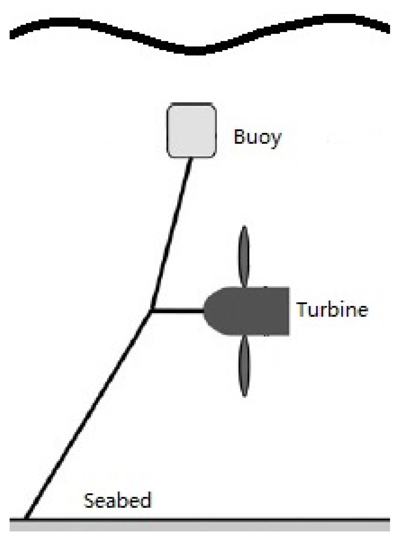
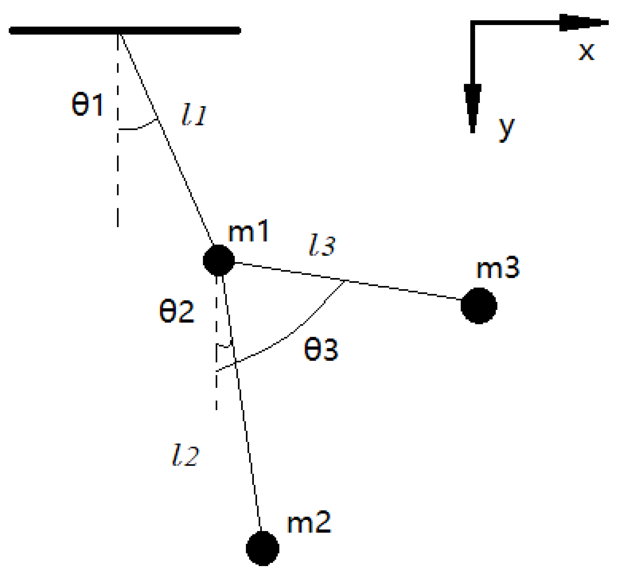
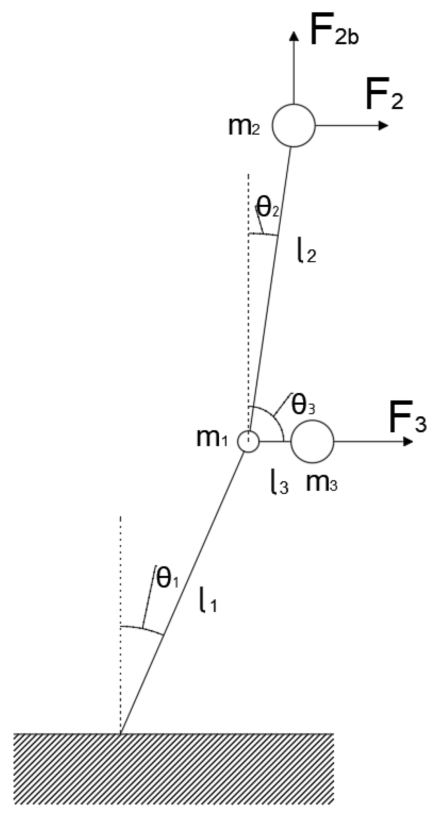
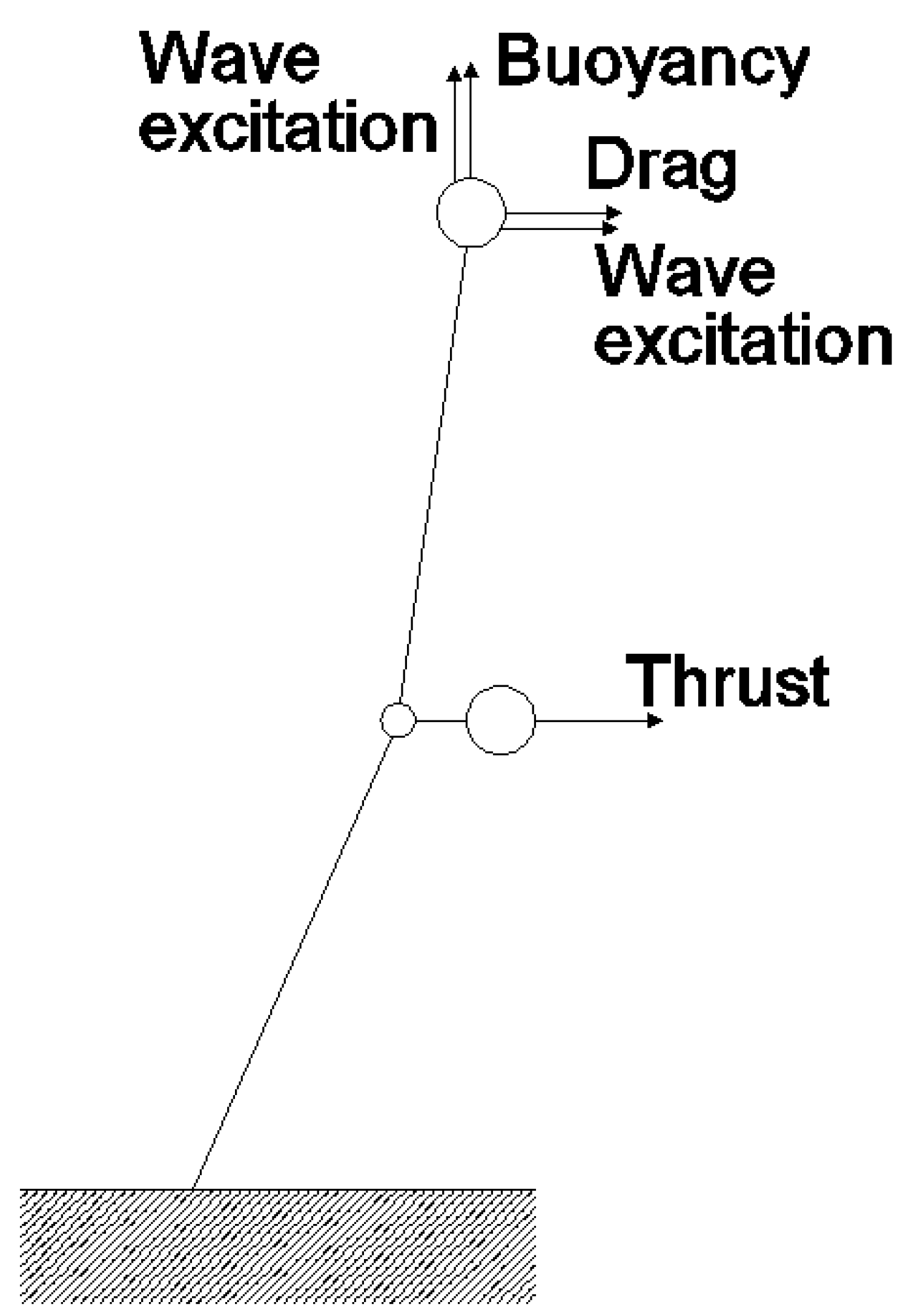
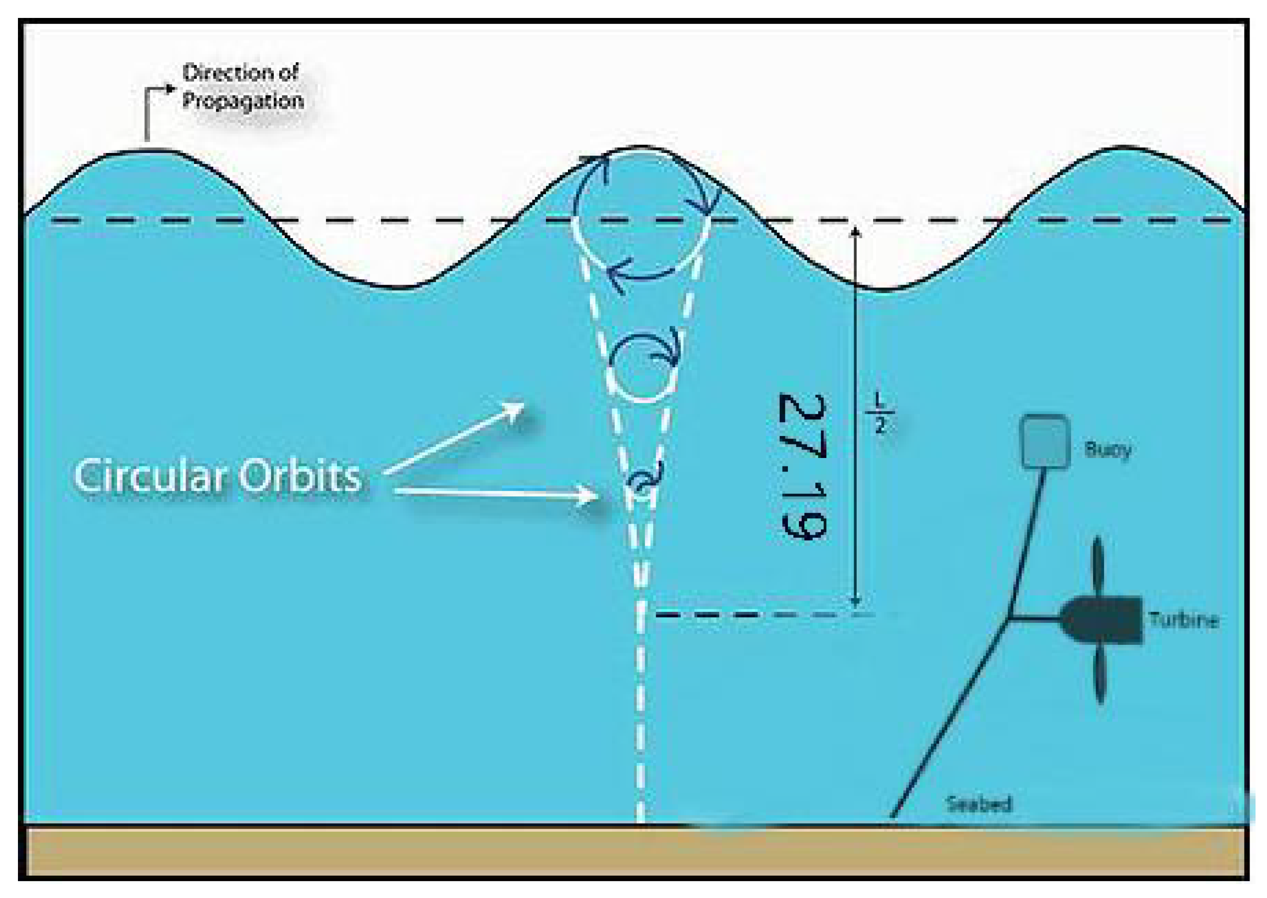
2.1. Model of Mooring Supported Turbine
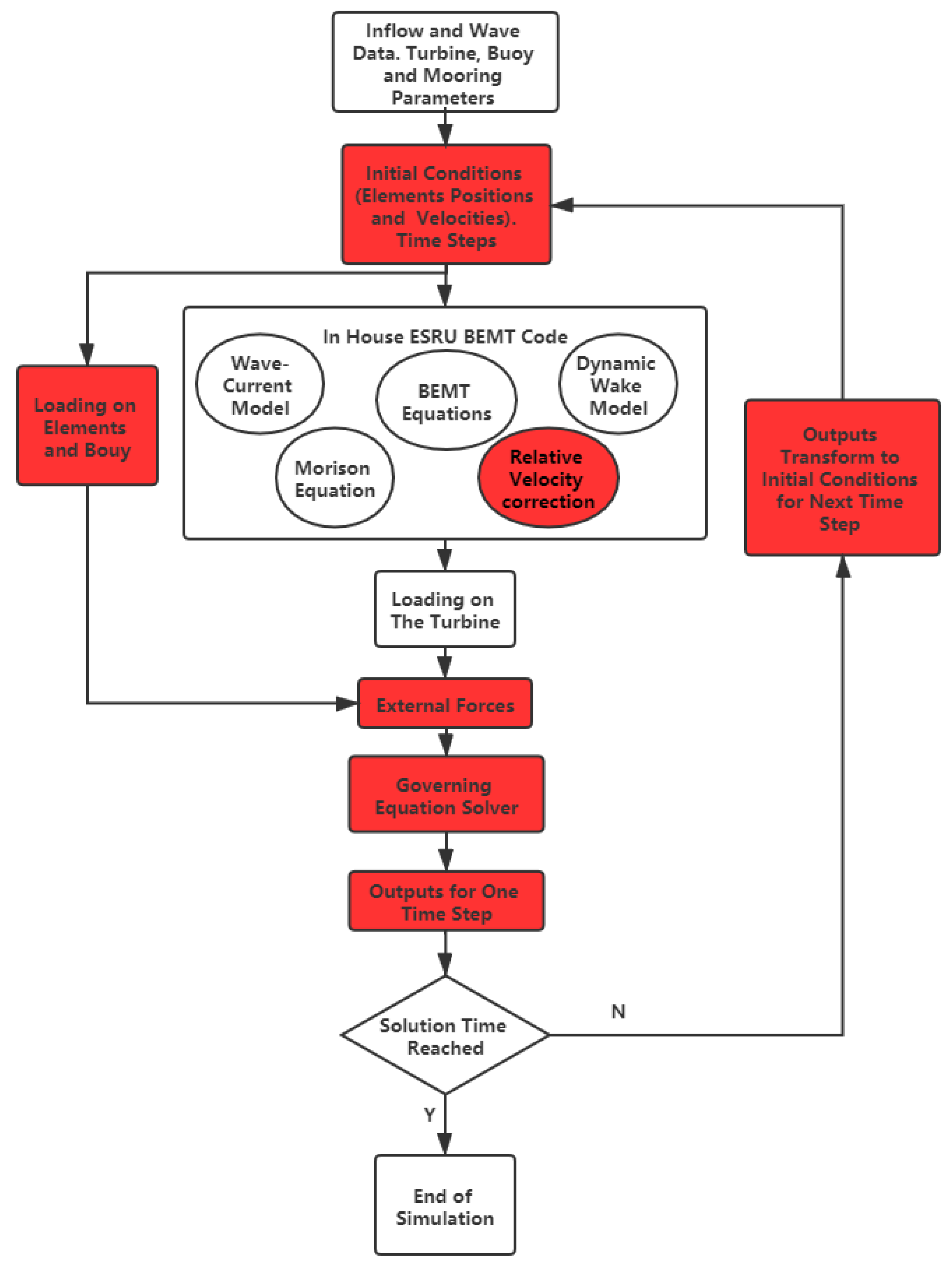
2.2. Flow Diagram
3. Initial Conditions and System Parameters
3.1. Initial Conditions
3.2. Sea States
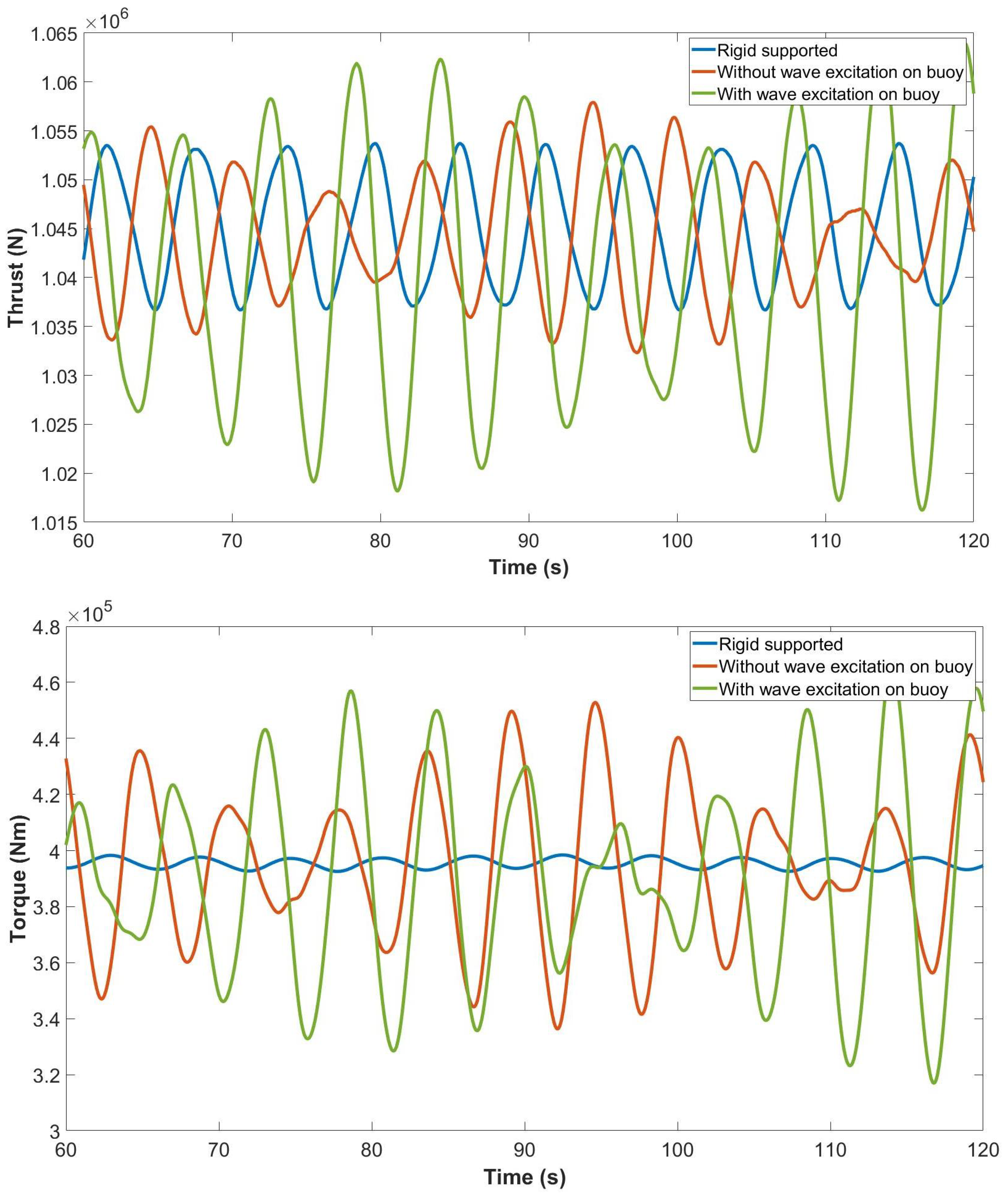
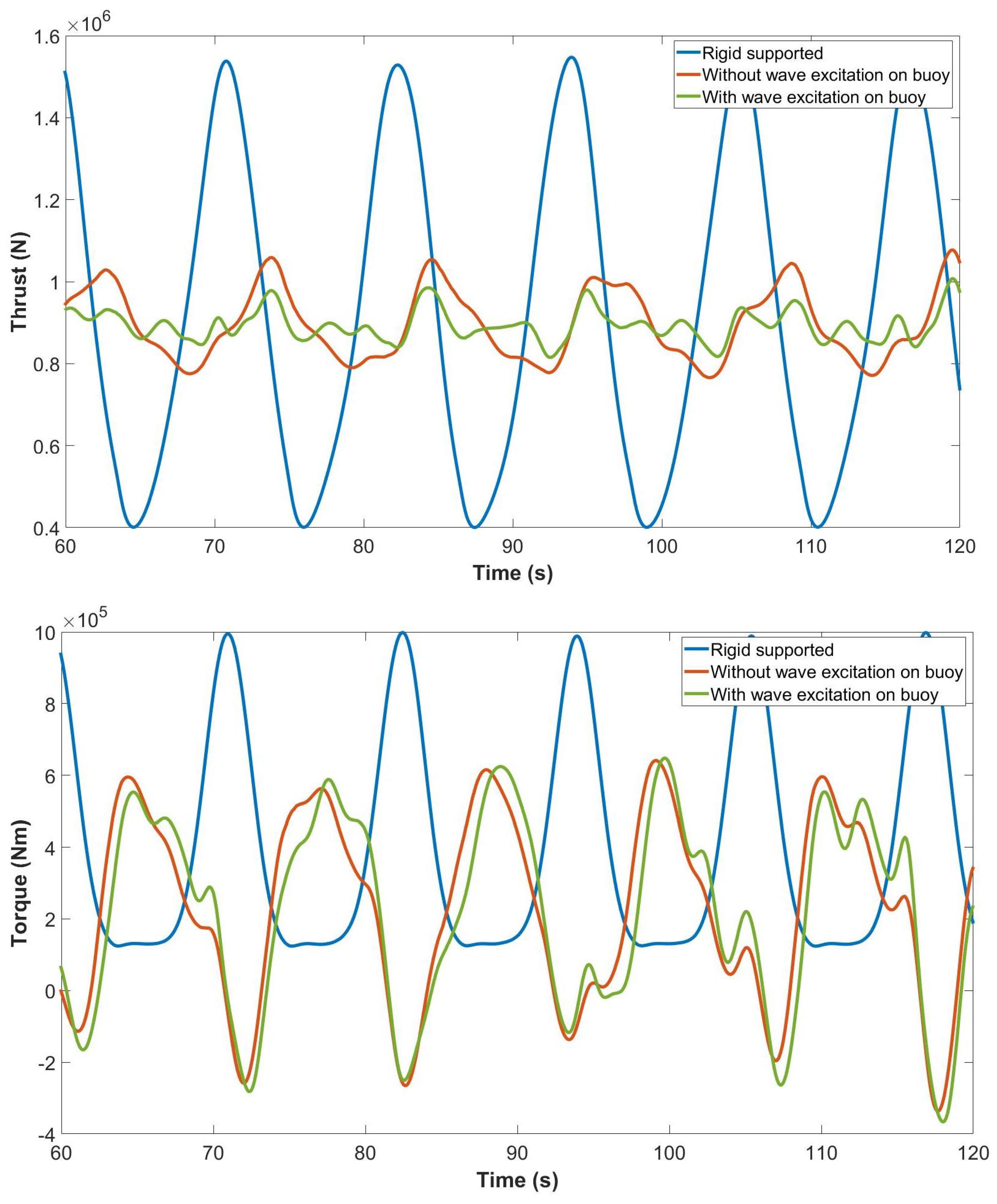
4. Results
5. Discussion
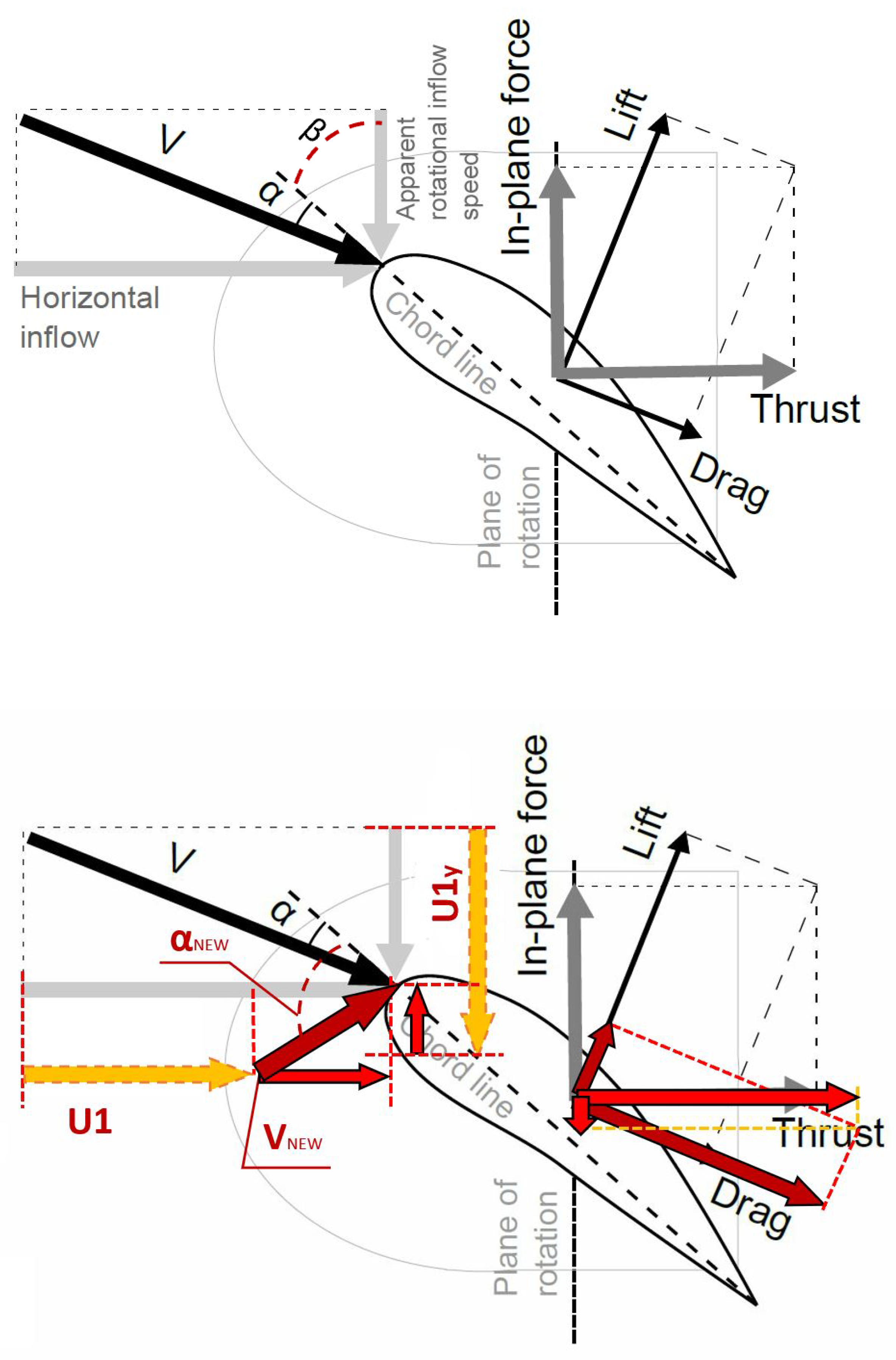
5.1. Blade Section Velocities
5.2. Wavelength Factor
5.3. Morison Effects
6. Conclusions
Author Contributions
Funding
Institutional Review Board Statement
Informed Consent Statement
Data Availability Statement
Acknowledgments
Conflicts of Interest
References
- Johnstone, C.; Pratt, D.; Clarke, J.; Grant, A. A techno-economic analysis of tidal energy technology. Renew. Energy 2013, 49, 101–106. [Google Scholar] [CrossRef]
- Simecatlantis. Projects. Available online: https://simecatlantis.com/projects/meygen/ (accessed on 13 June 2019).
- Emec Tidal Devices. Available online: http://www.emec.org.uk/marine-energy/tidal-devices/ (accessed on 30 September 2016).
- Clarke, J.A.; Connor, G.; Grant, A.; Johnstone, C.; Ordonez Sanchez, S. Contra-rotating marine current turbines: Single point tethered floating system—Stabilty and performance. In Proceedings of the 8rd European Wave and Tidal Energy Conference, Uppsala, Sweden, 7–10 September 2009. [Google Scholar]
- Huang, S. Dynamic analysis of three-dimensional marine cables. Ocean Eng. 1994, 21, 587–605. [Google Scholar] [CrossRef]
- Johanning, L.; Smith, G.H. Mooring design approach for Wave Energy Converter. J. Eng. Marit. Environ. 2006, 220, 159–174. [Google Scholar] [CrossRef]
- Smith, J.L. Station keeping study for wec devices including compliant chain, compliant hybrid and taut arrangement. In Proceedings of the 27th Offshore and Arctic Marine Engineering Symposium, Estoril, Portugal, 15–20 June 2008. [Google Scholar]
- Xu, S.; Wang, S.; Guedes Soares, C. Review of mooring design for floating wave energy converters. Renew. Sustain. Energy Rev. 2019, 111, 595–621. [Google Scholar] [CrossRef]
- Coiro, D.P.; Troise, G.; Bizzarrini, N. Experiences in Developing Tidal Current and Wave Energy Devices for Mediterranean Sea. Front. Energy Res. 2018, 6, 136. [Google Scholar] [CrossRef]
- Martynyuk, A.A.; Nikitina, N.V. The Theory of Motion of a Double Mathematical Pendulum. Int. Appl. Mech. 2000, 36, 1252–1258. [Google Scholar] [CrossRef]
- Nevalainen, T.; Johnstone, C.; Grant, A. An Unsteady Blade Element Momentum Theory for Tidal Stream Turbines. In Proceedings of the 11th European Wave and Tidal Energy Conference, Plymouth, UK, 5–9 September 2015. [Google Scholar]
- Maria Przybylska, W.S. Non-integrability of flail triple pendulum. Chaos Solitons Fractals 2013, 53, 60–74. [Google Scholar] [CrossRef]
- Nevalainen, T.; Johnstone, C.; Grant, A. A Sensitivity Analysis on Tidal Stream Turbine Loads Caused by Operational, Geometric Design and Inflow Parameters. Int. J. Mar. Energy 2016, 16, 51–64. [Google Scholar] [CrossRef]
- Elmas Anli, I.O. Classical and Fractional-Order Analysis of the Free and Forced Double Pendulum. Engineering 2010, 2, 935–949. [Google Scholar] [CrossRef][Green Version]
- Ohlhoff, A.P.R. Forces in the Double Pendulum. ZAMM J. Appl. Math. Mech./Z. Angew. Math. Mech. 2000, 80, 517–534. [Google Scholar] [CrossRef]
- Wu, G.; Witz, J.; Ma, Q.; Brown, D. Analysis of wave induced drift forces acting on a submerged sphere in finite water depth. Appl. Ocean Res. 1994, 16, 353–361. [Google Scholar] [CrossRef]
- Bossanyi, E. BLADED for Windows Theory Manual; Garrad Hassan and Partners Limited: Bristol, UK, 1997. [Google Scholar]
- Gaonkar, G.; Peters, D. Review of dynamic inflow modeling for rotorcraft flight dynamics. In Proceedings of the 27th Structures, Structural Dynamics and Materials Conference, Structures, Structural Dynamics, and Materials and Co-Located Conferences, San Antonio, TX, USA, 19–21 May 1986. [Google Scholar] [CrossRef]
- Schepers, J.G.; Snel, H. Final Results of the EU JOULE Projects Dynamic Inflow; Technical Report; U.S. Department of Energy Office of Scientific and Technical Information: Pasadena, CA, USA, 1996.
- Tuckerman, L.B. Inertia Factors of Ellipsoids for Use in Airship Design; Technical Report; US Government Printing Office: Washington, DC, USA, 1926.
- Buckland, H.; Masters, I.; Chapman, J.; Orme, J. Blade Element Momentum Theory in Modelling Tidal Stream Turbines. In Proceedings of the 18th UK Conference on Computational Mechanics, Southampton, UK, 8–10 April 2010. [Google Scholar]
- Chapman, J.C. Tidal Energy Device Hydrodynamics in Non-uniform Transient Flows. Ph.D. Thesis, Swansea University, Swansea, UK, 2008. [Google Scholar]
- Whelan, J.M.R.; Graham, J.P. Inertia Effects on Horizontal Axis Tidal-Stream Turbines. In Proceedings of the 9th European Wave and Tidal Energy Conference, Lincoln, NE, USA, 24–26 June 2009. [Google Scholar]
- Nevalainen, T. The Effect of Unsteady Sea Conditions on Tidal Stream Turbine Loads and Durability. Ph.D. Thesis, University of Strathclyde, Glasgow, UK, 2016. [Google Scholar]
- British Oceanographic Data Centre. Wave Data. Available online: https://www.bodc.ac.uk/data/online_delivery/waves/search/ (accessed on 30 September 2016).
- Simecatlantis. Simec Atlantis Energy Unveils World’S Largest Single Rotor Tidal Turbine, The AR2000. Available online: https://simecatlantis.com/2018/09/13/simec-atlantis-energy-unveils-worlds-largest-single-rotor-tidal-turbine-the-ar2000/ (accessed on 13 June 2016).
- Airfoil Tool. NREL’s S814 Airfoil (s814-nr). Available online: http://airfoiltools.com/airfoil/details?airfoil=s814-nr (accessed on 9 October 2021).
- ABP Marine Environmental Research Ltd. Atlas of UK Marine Renewable Energy. Available online: https://www.renewables-atlas.info/ (accessed on 15 August 2017).
- Fenton, J.D. A fifth-order Stokes theory for steady waves. J. Waterw. Port Coastal Ocean Eng. 1985, 111, 216–234. [Google Scholar] [CrossRef]


| Initial Conditions | ||
|---|---|---|
| System Parameters | |||
|---|---|---|---|
| 5 t | rotor rotation speed | 1.25 rad/s | |
| 80 t | airfoil profile | NRELs814 [27] | |
| 30 m | number of blade | 3 | |
| 15 m | mooring line segment length | 0.5 m | |
| 3 m | mooring line material | Dyneema | |
| buoy radius | 3 m | number of blade element | 20 |
| Sea States | 1 | 2 | 3 | Harsh Winter |
|---|---|---|---|---|
| [m] | 2.665 | 1.07 | 1.008 | 10.12 |
| [s] | 6.135 | 11.07 | 4.653 | 10.06 |
| water depth [m] | 50 | 50 | 50 | 50 |
| steepness (H/gT) | 0.0719 | 0.0099 | 0.0237 | 0.1027 |
| wave model | 3rd-order | linear | 2nd-order | 3rd-order |
Publisher’s Note: MDPI stays neutral with regard to jurisdictional claims in published maps and institutional affiliations. |
© 2021 by the authors. Licensee MDPI, Basel, Switzerland. This article is an open access article distributed under the terms and conditions of the Creative Commons Attribution (CC BY) license (https://creativecommons.org/licenses/by/4.0/).
Share and Cite
Fu, S.; Johnstone, C. Numerical Performance Model for Tensioned Mooring Tidal Turbine Operating in Combined Wave-Current Sea States. J. Mar. Sci. Eng. 2021, 9, 1309. https://doi.org/10.3390/jmse9111309
Fu S, Johnstone C. Numerical Performance Model for Tensioned Mooring Tidal Turbine Operating in Combined Wave-Current Sea States. Journal of Marine Science and Engineering. 2021; 9(11):1309. https://doi.org/10.3390/jmse9111309
Chicago/Turabian StyleFu, Song, and Cameron Johnstone. 2021. "Numerical Performance Model for Tensioned Mooring Tidal Turbine Operating in Combined Wave-Current Sea States" Journal of Marine Science and Engineering 9, no. 11: 1309. https://doi.org/10.3390/jmse9111309
APA StyleFu, S., & Johnstone, C. (2021). Numerical Performance Model for Tensioned Mooring Tidal Turbine Operating in Combined Wave-Current Sea States. Journal of Marine Science and Engineering, 9(11), 1309. https://doi.org/10.3390/jmse9111309