Assessment of Seasonal and Spatial Variations of Coastal Water Quality Using Multivariate Statistical Techniques

Abstract

This study investigates the seasonal and spatial trends in Kuwait’s coastal water’s physical, chemical, and biological parameters by applying multivariate statistical techniques, including cluster analysis (CA), principal component/factor analysis (PCA/FA), and the Pearson correlation (PC) method to the average daily reading of water quality parameters from fifteen stations over one year. The investigated parameters are pH, turbidity, chlorophyll-a, conductivity, dissolved oxygen (DO), phycoerythrin, salinity, and temperature. The results show that the coastal water of Kuwait is subjected to high environmental pressure due to natural and human interferences. During 2017, the DO levels were below the threshold limit, and at the same time, the water temperature and salinity were very high, causing a series of fish death events. CA resulted in three different regions based on the turbidity, including high, moderate, and low regions, and three seasons (winter, summer, and autumn). Spring is very short and overlaps with winter and summer. PCA/FA applied on the datasets assisted in extracting and identifying parameters responsible for the variations in the seasons and regions obtained from CA. Additionally, Pearson’s correlation resulted in a strong positive relation between chlorophyll and phycoerythrin in 7 out of the 15 stations. However, at high turbidity regions (stations 1 and 2), chlorophyll concentration was low. Additionally, the negative correlation between DO and temperature was observed at stations with rare human activities.

1. Introduction

Coastal waters are the linkage between land and sea/ocean as it provides several activities performed by humans, such as transportation, tourism, and fisheries. They represent 0.5% of the ocean volume and occupy up to 10% of the ocean surface [1]. Coastal basins are an ultimate natural system for productivity on earth, and the coastal zone (100 km off the coast) is a preferable place for living for more than 40% of the world population [2]. Thus, coastal regions are of great economic, nutritional, and security importance; however, on the other hand, these areas are susceptible to human activities and climate change in terms of environmental impacts [1,3,4]. Environmental indicators have been degrading severely due to natural and human interventions over the past decades leading to a significant threat to the marine life and coastal ecosystem [5,6,7,8,9].

Releasing pollutants from outfalls, overfishing, and accidental events, such as oil spills, are examples of environmental threats to coastal water quality [3,10]. Hence, appropriate environmental management and development strategies are essential to restore and maintain ecosystem health and ecological services [11]. Continuous marine environment monitoring is thus essential to identify water quality issues such as red tides and hypoxia, as well as identifying harmful algae blooms and sediment plumes. In addition, reliable and continuous monitoring is helpful for researchers and decision-makers to characterize coastal basins temporally and spatially and identify the changes and trends of water properties [12].

Overall, the factors responsible for coastal water contamination cover chemical, physical, and biological characteristics [13]. These factors include chemical contaminants resulting from, for example, industrial waste, agricultural runoff, and nutrients and pathogens originating from, for example, overflows, stormwater, and sewage discharge. Besides the waste input from the outfalls, other factors such as rivers, creeks, and climate conditions contribute to changing water properties, specifically salinity and temperature.

Kuwait has experienced an increasing load on the marine environment, specifically within Kuwait Bay, due to several activities practiced in that region. The bay is a prime location for the spawning and nursery of different marine species, and until the end of the first half of the last century, it was Kuwaiti’s primary source of living and occupation [14]. However, due to the wide range of continuous developments applied along Kuwait’s coastline since the 1970s, Kuwait’s coastal water was subjected to environmental stresses that caused permanent harmful effects and allowed for hazardous environmental events. Such developments include urbanization, oil spills, discharges from power plants and sewage outfalls, climate change, and desalination [15,16,17,18,19,20]. These detrimental outcomes have led to the formation of red tides and large quantities of fish kill events that occurred in 1999 and 2001, and also in recent years [21,22,23,24,25,26].

Several studies have been conducted regarding the appearing issues, and through which they focused on spatial analysis to monitor Kuwait’s water quality using multivariate and geostatistical techniques. These studies (e.g., [16]) showed that the monitoring networks are insufficient to show the different water quality patterns and inadequate for the heavily polluted areas. Nicolaus and others [27] assessed the temporal and spatial variations of the total petroleum hydrocarbons (TPHs) and nine other metals from measured data from 23 locations within the territorial coastal water of Kuwait between 1984 and 2017. During the study period, their findings showed a violation of the Kuwaiti assessment criteria for two metals, cadmium (Cd) and copper (Cu). Suggestions have been made for further monitor and sampling, focusing on specific locations like the shorelines and the bay. Chen and others [14] analyzed the variation of Kuwait Bay’s fish abundances and assemblages spatially and temporally. Their results showed that the fish abundance varies temporally, and the fish assemblages vary spatially. The temporal variation of fish abundance could be due to the changes in the water quality parameters.

Kuwait Environment Public Authority (KEPA) has monitored the water quality of Kuwait’s coastal and offshore waters through 15 floating buoys since 2016 (Figure 1). These buoys were deployed as part of a monitoring program for the marine environment in Kuwait, northwest of the Arabian Gulf. The spatial distribution of the buoys allows researchers to investigate the variation in water quality parameters temporally and spatially. Most previous studies either cover the spatial or temporal variations or include both but consider limited parameters.

The Environment Public Authority has entrusted the managing and operating of the monitoring stations to one of the local environmental companies. However, in July 2018, these stations were stopped because the data extracted from them was labeled as illogical data by KEPA. For example, the salinity in Kuwait is very high, above 40 psu, yet the recorded salinity was consistently below 25 psu. Accordingly, after analyzing the previous data by KEPA, all illogical data were removed, and only the daily average data for the year 2017 was approved and used in this study.

This study investigates seawater parameters’ seasonal and temporal trends using complete daily average data of 2017 of available parameters. These parameters include the pH, turbidity, chlorophyll-a, conductivity, dissolved oxygen (DO), phycoerythrin, salinity, and temperature. Different statistical approaches were applied to decompose the bay into regions and identify possible relationships between the parameters. Such decomposition and relationships distinctively aim to check the effectiveness and reliability of the identified water patterns recorded, which is considered a competitive advantage over previous studies in the same region.

2. Methodology

2.1. Study Area

The study area covers the entire coastal waters of Kuwait from the southern region to the northern region, as shown in Figure 1. The names and coordinates of the 15 monitoring stations and the water depth at each station are listed in

Table 1. Station names and coordinates.

Buoy ID	Name	Longitude	Latitude	Water Depth at Mean Sea Level (m)
St-01	Southeast of Ras Al-Khaid (Babayan Island)	48.461675	29.724966	4.7
St-02	Khor Babayan	48.033614	29.916501	3.3
St-03	Khor Al-Sabiya Entrance (SE Ras Al-Barsha)	48.322461	29.542470	2.2
St-04	Northeast of Ras Azujha	48.058310	29.461648	9.5
St-05	Northeast of Doha Port	47.908330	29.459927	6.1
St-06	Northeast of Doha Port	47.833326	29.421614	10.3
St-07	West of Doha Port	47.791731	29.391653	6.0
St-08	West of Al-Akaz	47.880965	29.364121	3.6
St-09	Southeast of Al-Beda’a	48.108565	29.276854	15.8
St-10	Northeast of Nort Pier (Ahmadi Port)	48.333389	29.233381	8.3
St-11	Southeast of Abdulla Port	48.183245	29.000013	6.7
St-12	Northeast Kubbar Island	48.491826	29.091657	27.1
St-13	Southwest of Quroh Island	48.743612	28.799867	28.9
St-14	Northeast of Um Al-Maradim Island	48.660620	28.686551	12.8
St-15	Southeast Mina Az-Zour	48.441634	28.691583	12.7

. Stations 4 to 8 are located within Kuwait Bay, rich in marine life diversity and many environmental issues. Station 2 is located south of Khor Al-Zubair estuary, which discharges less than 10 m³/s of water to the Arabian Gulf during ebb tide [28,29]. The bottom bed of the area where stations 1, 2, and 3 are located consists of cohesive sediments with 15% sand, 25% clay, and 60% silt [29,30]. The amount of suspended solids in this area is 0.832 g/L during ebb tide and 0.612 g/L during flood tide. Stations 9–15 are located in the open sea at deeper water and have fewer environmental stressors.

2.2. Data Parameters

The collected data includes eight parameters defined and presented in

Table 2. Defined coastal water quality parameters.

Parameter	Unit	Description and Characteristics
pH	-	Represent the acidic or essential nature of the water
Turbidity	NTU	Occurs based on particles that are bigger than 2 microns (suspended solids)
Chlorophyll-a	mg/m3	The green photosynthetic pigment in algae, cyanobacteria, plants
Conductivity	mS/cm	The liquid’s ability to deliver electricity
Dissolved oxygen	mg/L	Represent the level of free oxygen in the water
Phycoerythrin	ppb	Red protein pigment complex
Salinity	PSU	Represent the dissolved inorganic salt content on the water.
Temperature	°C	Water temperature measurement

. First, T•Xchange and Tu•Xchange by AML were used to measure water temperature and turbidity. The Tu•Xchange measures the turbidity accurately up to 3000 NTU. Second, the dissolved oxygen is measured using Oxygen Optode/Temperature Sensor 4130, which is designed to operate in a water temperature range between 0–40 °C and water depth in the range between 0–300 m. Third, the temperature, conductivity, and salinity were measured using the AML CT•Xchange, which calculates the temperature and salinity in the range between 0–40 °C and 0–70 PSU, respectively. Finally, the pH, chlorophyll-a, and phycoerythrin were measured using X2change by AML. The instrument range for pH is 0–14, for chlorophyll-a is 0–500 μg/L, and for phycoerythrin is 0–750 ppb. As mentioned earlier, all these instruments are operated and maintained (calibrated) by a local environmental company. The maximum, mean, and minimum of each parameter in all stations are shown in Figure 2.

2.3. Data Analysis

2.3.1. Data Exploration

The available data were analyzed using IBM SPSS Statistics 26. First, the results were compared with the standard limits of KEPA (

Table 3. Standard limits of KEPA for some of the study’s parameters.

Parameter	Limits
pH	6.5–8.5 (Maximum)
Turbidity	75 NTU (Maximum)
Chlorophyll *
Dissolved oxygen	4 mg/L (Minimum)
Salinity	45 psu

* The limits are not specified by KEPA bylaws.

), and the values that exceeded the standard limits were specified. Then a frequency tool was used to count these values and calculate their percentage from the total value for each parameter. Finally, multivariate analysis tools were used to study spatial and temporal behavior for each parameter in this study.

2.3.2. Cluster Analysis (CA)

The investigation and review of data are being reformed into various most popular techniques to handle the assessment of the wide-ranging amount of data such as environmental and water quality data. Cluster analysis (CA) is one of the multivariate analysis methods used for data classification and grouping and is recognized as one of the significant applications in environmental modeling. Hierarchical CA combines similar cases into groups (clusters) and results in a dendrogram graph visually representing the clusters formed. CA measures similarity using the squared Euclidean distance on normalized data using Ward’s method [31]. In this study, CA was performed based on the spatial location of station sites to determine similarities related to location. Regarding temporal variation, CA was performed according to the months of the year to identify parameter seasonality.

2.3.3. Principal Component Analysis

Principal component analysis (PCA) is used to reduce a multivariate dataset’s dimensionality while maintaining the original data’s complete information. PCA operates by creating a non-correlated component consisting of subsets from the original data. The variance in the original dataset is identified as new pseudo-variables called principal components [32]. The PCA is expressed as [31]:

$$z_{\mathrm{i}\mathrm{j}}={\mathrm{pc}}_{\mathrm{i}1}{\mathrm{x}}_{1\mathrm{j}}+{\mathrm{pc}}_{\mathrm{i}2}{\mathrm{x}}_{2\mathrm{j}}+{\mathrm{pc}}_{\mathrm{i}3}{\mathrm{x}}_{3\mathrm{j}}+\dots +{\mathrm{pc}}_{\mathrm{im}}{\mathrm{x}}_{\mathrm{mj}}$$

(1)

In Equation (1), z is the component’s score, pc is the loading of the component, x is the measured value, i is the component number, j is the sample number, and m is the total number of variables.

2.3.4. Pearson Correlation Coefficient

The relationship between water parameters is assessed using Pearson’s correlation coefficient. This coefficient ranges between −1 and 1, and as it becomes closer to the absolute value of 1, the relationship between the parameters becomes stronger. The Pearson correlation coefficient is given by:

$$r_{xy}=\frac{{{\displaystyle \sum }}_{i=1}^n\left(x_i-\overline{x}\right)\left(y_i-\overline{y}\right)}{\sqrt{{{\displaystyle \sum }}_{i=1}^n{\left(x_i-\overline{x}\right)}^2}\sqrt{{{\displaystyle \sum }}_{i=1}^n{\left(y_i-\overline{y}\right)}^2}}$$

(2)

where x and y are two different water parameters, $i$ and $j$ are the samples’ numbers, $\overline{x}$ and $\overline{y}$ are the means of the two parameters, and $n$ is the number of data points. The Pearson’s correlation coefficient sign determines whether the relationship between the parameters is linearly proportional or inversely proportional [33,34]. In this study, Pearson’s correlation coefficient is used to determine the relationship between different water parameters.

3. Results and Discussion

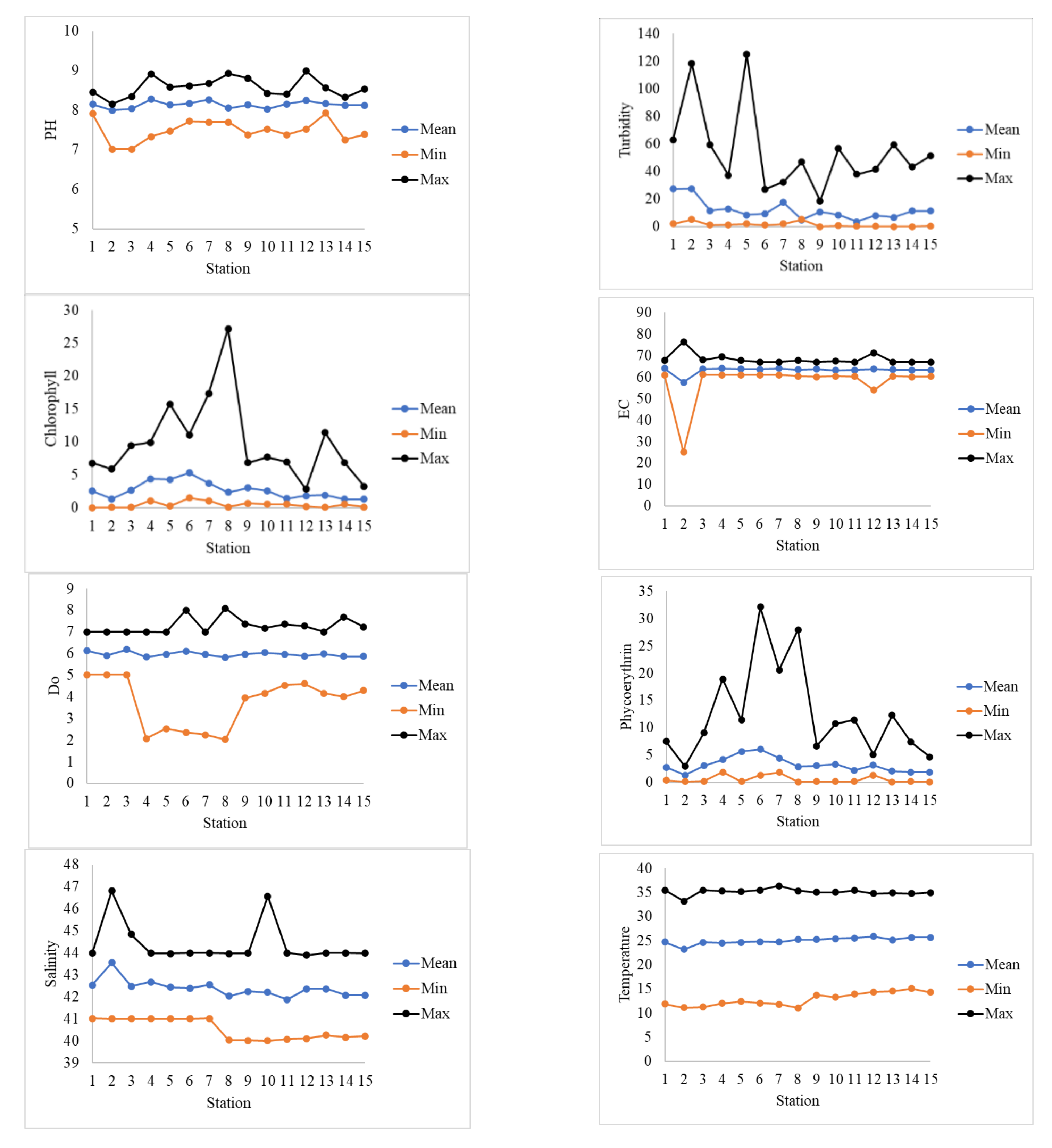
The basic statistics of the water quality parameters of this study are shown in Figure 2. The figure shows that the maximum, mean, and minimum values of the pH for all stations are within the standard limits of KEPA (Table 3). These values indicate that the acidity of the water is neutral, and no threat exists to the biological life. The maximum pH value was 8.98 and recorded at station 12, while the minimum value was recorded at two stations, St-02 and St-03, with a value of $\approx 7$.

The turbidity varies widely between stations and for the same station. The maximum turbidity was at station 5 with a value of 125 NTU (exceeds KEPA maximum limit), and the minimum was nearly 0 at stations 9–15. Stations of high turbidity are either located in areas of cohesive beds (St-02 and ST-05) or located in areas where there are frequent waste discharges from coastal outfalls. The highest mean turbidity values were observed at stations ST-01 and ST-02, where continuously suspended nutrients and fine sediments are discharged from the northern rivers (e.g., Shat Alarab and Khor Abdullah).

The DO levels in coastal water are significant for human and marine life health. Within Kuwait’s coastal water, the DO ranges between 2 and 8 mg/L (Figure 2). These low values are below KEPA, and the international standards of the minimum DO level, and all occurred within Kuwait bay. Many factors cause these low levels of DO within the bay, but it is mainly due to weak flushing characteristics of the bay and the existence of more than ten primary sewage and brine outfalls along the southern coast of the bay. The times when the dissolved oxygen level fell to minimum levels witnessed four fish death events off the southern coast of Kuwait Bay. The average value of the DO at all stations is nearly 6 mg/L which is above the minimum KEPA limits, which is acceptable for the safety of marine species.

The coastal water of Kuwait and the Arabian Gulf, in general, is known for its high temperature and salinity. The mean salinity at all stations in 2017 was between 41.9 psu (ST-11) and 43.6 psu (ST-02). The maximum salinity level was $\approx$47 psu at St-02, and the minimum was ≈40 psu at stations St-08–St-15. These high salinity levels are due to the extensive amount of desalination plant outfalls along the Arabian Gulf coastline, extreme arid weather, and slow flushing characteristics of the Arabian Gulf and specifically within Kuwaits’ coastal water. High salinity contributes significantly to many coastal environmental, health, and economic issues [35].

The water temperature ranges between 11.1 °C in winter and 36.4 °C in summer. Comparing the DO and temperature data, it was noticed that the lower DO levels occurred in summer when the temperature was very high. This result agrees with the known fact that warm water holds less DO [31,36]. Heil and Glibert and others [24,37] reported that high temperature levels were the leading cause of the major fish kill event in the summer of 2001.

The above statistics of some water quality parameters show that the coastal water of Kuwait is subjected to potential environmental pressure. This pressure is mainly due to high levels of temperature and salinity and low levels of DO. The causes of the potential threats are due to either natural processes, such as climate change, or due to human inferences, such as oil spills, waste discharge, desalination plants’ discharge, and aggressive fishing.

It is essential to realize that some of the water parameters are dependant on each other, and they vary seasonally and spatially. As mentioned earlier, cluster analysis (CA) and principal component/factor analysis (PCA/FA), and Pearson correlation (PC) are frequently used in water quality studies in coastal areas to study the seasonal and spatial variations of water properties. The daily average water quality data is analyzed next using the above three analyses.

3.1. CA

The CA identified the data into discrete groups with similar characteristics where they are closely associated. CA handled both locational and seasonal variations as presented below.

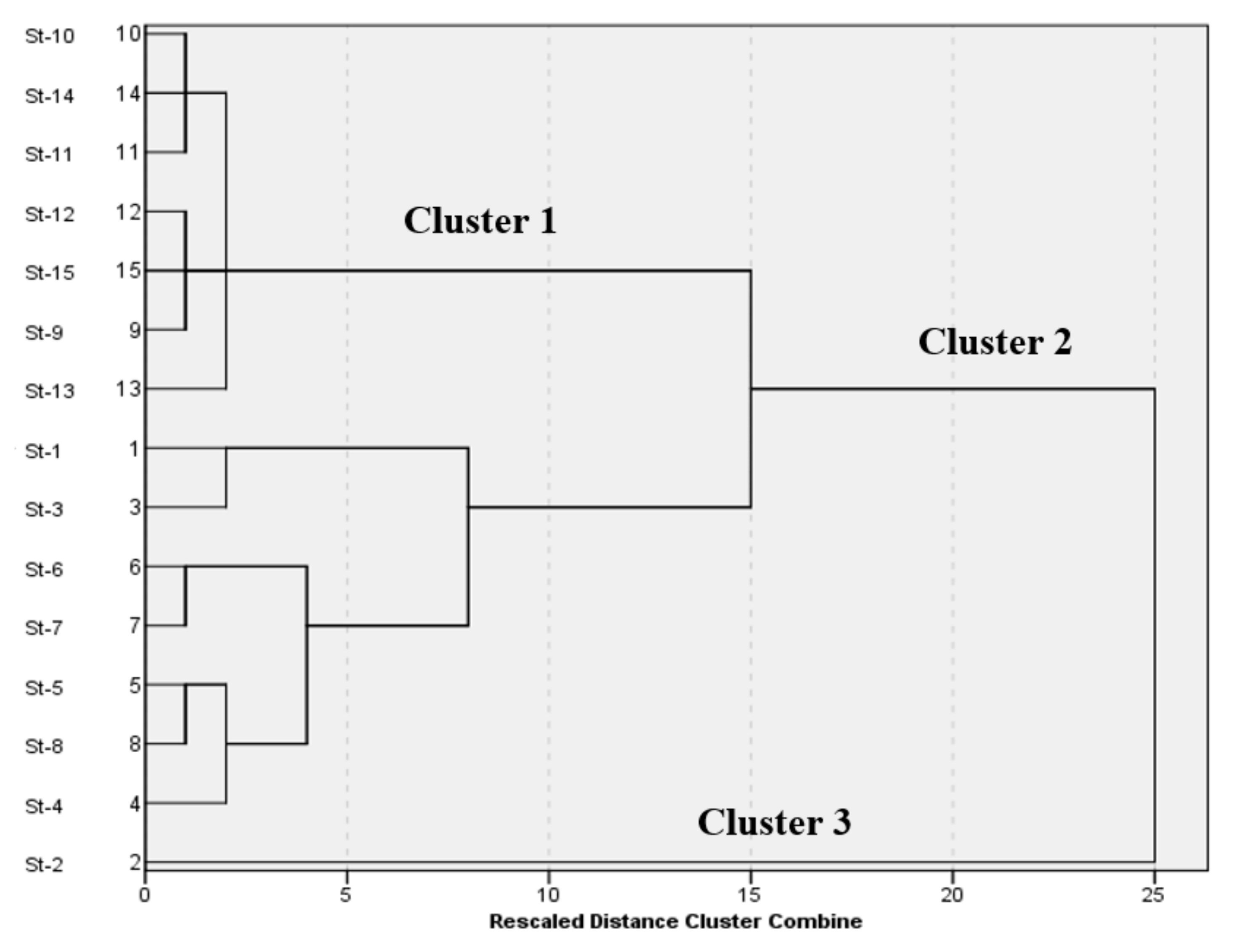
The locational CA characterized the similarity within the 15 stations included in this study. The analyzed data employed the mean values of seawater parameters and resulted in three clusters, as shown in Figure 3, at (D_link/D_max) $\times$ 100 < 40. From the mean turbidity values for each station, it is inferred that CA has grouped the stations based on turbidity, and hence, the three groups are classified as high turbidity (HT), medium turbidity (MT), and low turbidity (LT). The LT region includes seven stations and is represented by Cluster 1, which combines station 9 to station 15 and is located in Kuwait’s southern region. Additionally, the MT region, called Cluster 2, combines station 1 and station 3 to station 8 and is generally indicated as Kuwait Bay. Lastly, Cluster 3 includes only station 2 while representing the HT area, occupying the northern region of Kuwait and Boubyan Island, as previously shown in Figure 1.

The high turbidity values in the HT region, including station 2, are due to the shallow water levels that receive silt and clay from Khor Abdallah [29,38]. In addition to that, station 2 shows high salinity values related to low water circulation in this region [39]. The MT region covers the stations near human activities such as fishing and industrial ports. Such activities cause an increase in chlorophyll-a and phycoerythrin values and lead to an increase in the concentration of nutrients in seawater [40]. Finally, the LT region is located on the south coast of Kuwait and is characterized as open water. In such regions, the water circulation is higher, and the turbidity values are low.

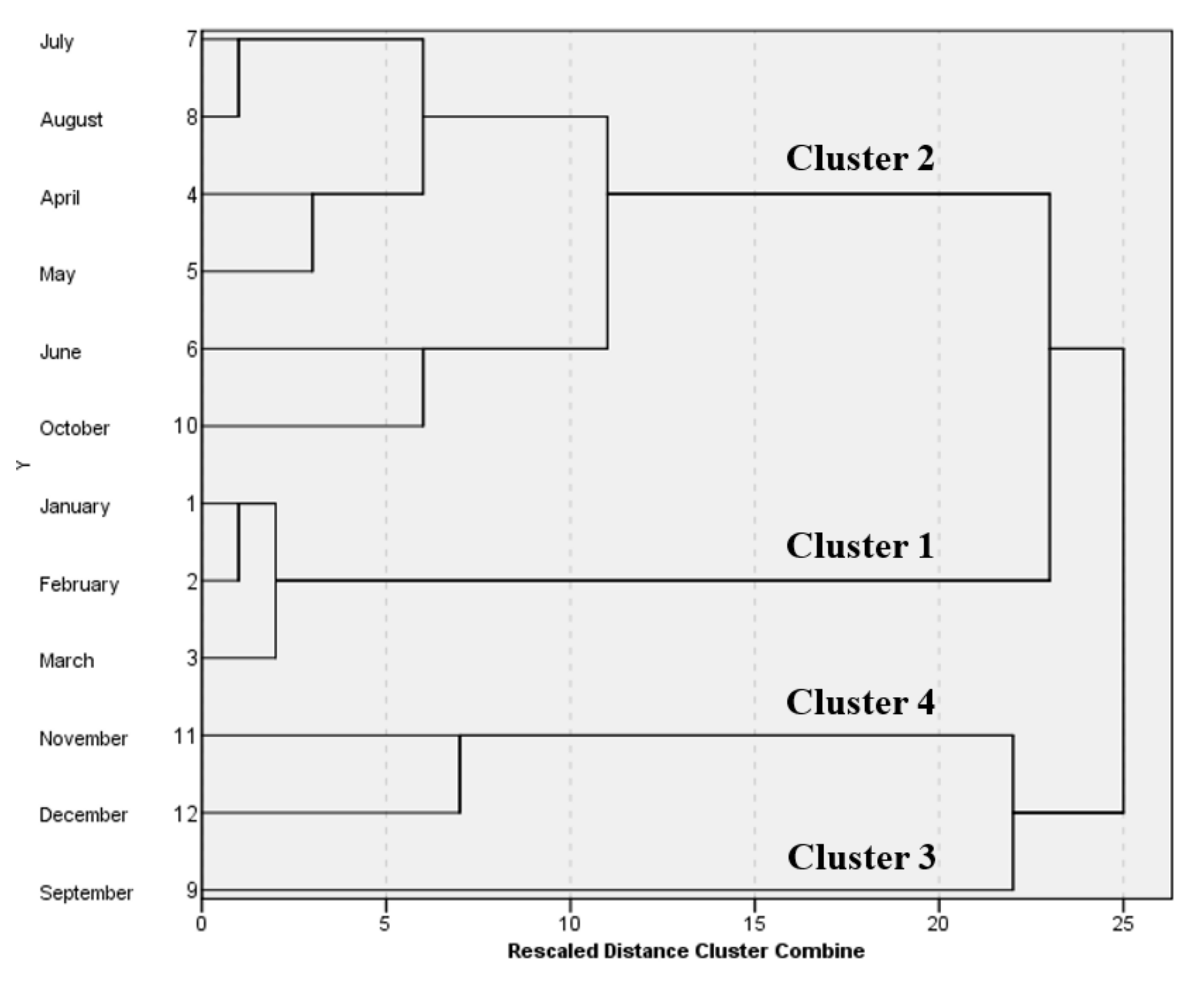
The seasonal variations concerning the coastal water quality values were investigated using the CA method, including the 12 months (January–December) of 2017. The analysis resulted in four significant clusters at (D_link/D_max) $\times$ 100 < 60, as shown in Figure 4. Although there are four clusters, it is observed that Cluster 3, which includes the month of September only, lies in between months classified as Cluster 2 (from April to August and October). Such conflict and shifting between October and September result from seasons transition, in which the temperature range in September 2017 was 24–47 °C, while in October 2017, the temperature recorded was in the range of 16–43 °C. Similarly, in 2018 and 2019, the recorded temperature ranged between 25–48 °C and 23–48 °C for September, and 13–43 °C and 20–45 °C for October [41]. Hence, Cluster 2 and 3 were combined as the analyzed data fitted the values of April–August and October in the summer season. Hence, CA on temporal variation resulted in three seasons, which are winter, summer, and autumn. Spring is very short and overlaps with winter and summer. Cluster 1 combines the months from January to March, referring to the winter season. Additionally, Cluster 4 represents the autumn season which includes November and December.

Kuwait is known for its extreme weather conditions, such as high temperatures in spring and autumn, and the CA resulted in the summer season, ranging from April to October. Similarly, Polikarpov and others [42] have performed temporal analysis on Kuwait gulf water from October 2005 to September 2006, and their results showed similar clustering with three main seasons: late-winter–spring, summer–early-autumn, and late-autumn–winter.

3.2. Principal Component/Factor Analysis (PCA/FA)

This method was applied to the available data set, including eight variables to identify and accentuate the seasonal and locational variability of the water samples’ compositional patterns. As defined by CA, PCA/FA was carried out in three different regions: HT, MT, and LT; and in three seasons: winter, summer, and autumn. The PCA/FA data input matrices (variable x cases) accounted for (8 × 2555) regarding LT and MT regions. However, the data input matrix for the HT region was (8 × 365). Additionally, the analyzed data resulted in three seasons for the seasonal variations: winter, summer, and autumn. Therefore, the data input matrices included (8 × 1260) for winter, (8 × 2996) for summer, and (8 × 854) for autumn.

PCA results were considered accounting for an Eigenvalue greater than 1, and the values of the factor loadings are classified in the ranges of > 0.75, 0.75–0.50, and 0.50–0.30, referred to as strong, moderate, and weak, respectively. Moreover, for the three regions investigated, the LT region yielded four PCs, explaining a total variance of 71.26% in correspondence to the water quality data sets. The MT region resulted in three PCs with a total variance of 57.31%, and the HT region explained a total variance of 64.95%, accounting for the two PCs generated.

Table 4. Loadings of experimental variables (8) on significant principal components for low turbidity (LT), medium turbidity (MT), and high turbidity (HT) regions.

	pH	Turbidity	Chlorophyll	EC	DO	Phycoerythrin	Salinity	Temperature	Eigenvalue	Variance %	Cumulative %
LT Region
PC1	−0.013	0.097	−0.531	0.796	−0.011	−0.54	0.815	−0.264	1.95	24.378	24.378
PC2	0.442	0.027	0.644	0.476	−0.01	0.68	0.455	0.144	1.528	19.101	43.479
PC3	0.58	0.657	−0.245	−0.107	−0.289	−0.155	−0.073	0.487	1.19	14.879	58.358
PC4	0.096	0.504	0.061	−0.045	0.821	0.003	−0.057	−0.293	1.032	12.9	71.26
MT Region
PC1	−0.146	−0.841	0.901	−0.609	−0.16	0.94	0.599	0.578	3.514	43.924	43.924
PC2	0.542	−0.078	−0.01	−0.287	0.813	0.084	0.458	−0.65	1.682	21.023	64.95
HT Region
PC1	−0.442	−0.16	0.535	0.604	−0.25	0.624	0.562	0.391	1.792	22.397	22.397
PC2	0.062	0.075	0.464	0.07	0.796	0.14	0.261	−0.733	1.489	18.613	41.01
PC3	0.343	0.357	−0.303	0.592	−0.064	−0.516	0.587	−0.028	1.304	16.3	57.31

summarizes the results obtained by PC analysis.

Furthermore, PC1, regarding the LT region, explained 24.38% of the total variance and had strong positive loading on electrical conductivity (EC) and salinity. The relationship between salinity and EC is explained by ions that increase the conductivity of water. Therefore, PC1 might be representative of impact desalination discharge along the southern coast of Kuwait. Moreover, PC2, covering 19.1% of the total variance, has a moderate positive loading on chlorophyll-a and phycoerythrin, which means that this component represents algae or simple aquatic organisms’ impact. Moderate turbidity and positive pH loading are present in PC3, representing water and reef fish aggregation [43]. PC3 explains 14.88% of the total variance of the LT cluster. The last component in LT is represented by PC4, explains 12.9% of the total variance, and has strong positive loading on DO, indicating the impact of nutrients and biological organisms [38].

PC analysis on the MT cluster resulted in PC1 and PC2, which explains 43.92% and 21% of the total variance. As the MT region lies in a closed bay area with heavy cargo traffic, which causes increased turbidity, PC1 has a strong negative loading on turbidity and a strong positive loading on chlorophyll-a and phycoerythrin. The negative relationship between turbidity and chlorophyll-a/phycoerythin is explained by large ships’ movement that causes turbidity in water and harms the algae and aquatic life. Additionally, PC2 has strong positive loading on DO, indicating the impact of nutrients and biological organisms.

As for the HT region, PC1 explains 22.4% of the total variance of the data and has moderate positive loading on chlorophyll-a, phycoerythrin, EC, and salinity. Thus, PC1 can indicate the effect of water flow from Shat al Arab delta, reducing the region’s salinity and inversely affecting the aquatic organism population. PC2 explains 18.61% of the total variance of HT region data. Strong positive turbidity and moderate negative temperature loading exist in PC2, indicating the factor representing the impact of nutrients and biological organisms in this region. The inverse relationship between DO and temperature is due to the low solubility of oxygen in water at high temperatures [44]. Moreover, PC3 explains 16.3% of the total variance and experiences moderate positive loading on salinity and EC, and moderate negative loading on phycoerythrin.

On the other hand, the three seasonal variabilities shown in

Table 5. Loadings of experimental variables (eight) on significant principal components for winter, summer, and autumn.

	pH	Turbidity	Chlorophyll	EC	DO	Phycoerythrin	Salinity	Temperature	Eigen Value	Variance %	Cumulative %
Winter
PC1	−0.362	0.198	0.548	0.771	−0.104	0.597	0.784	−0.252	2.11	26.37	26.37
PC2	0.516	0.289	−0.553	0.498	0.272	−0.6	0.489	−0.206	1.619	20.24	46.61
PC3	−0.074	0.045	0.119	0.056	0.748	0.065	0.098	0.722	1.119	13.99	60.60
Summer
PC1	0.45	0.237	0.699	0.551	0.076	0.653	0.571	0.279	1.887	23.592	23.592
PC2	−0.269	0.227	−0.404	0.668	−0.041	−0.48	0.671	−0.307	1.51	18.877	42.47
PC3	0.262	0.653	0.038	−0.212	0.638	−0.034	−0.109	−0.528	1.24	15.502	57.97
Autumn
PC1	−0.253	0.061	0.854	−0.101	0.449	0.833	0.178	−0.45	1.936	24.204	24.204
PC2	−0.078	−0.181	−0.252	0.708	0.367	−0.264	0.812	−0.42	1.643	20.543	44.747
PC3	0.779	0.665	0.16	0.085	−0.206	−0.071	0.077	−0.371	1.273	15.912	60.66
PC4	−0.006	−0.016	0.26	0.534	−0.629	0.364	0.29	0.534	1.25	15.621	76.28

yielded three PCs for the winter season with a total variance of 60.6% for the water quality datasets. However, a total variance of 57.97% was interpreted for the three PCs obtained regarding the summer season. As for the autumn season, the four PCs explained a total variance of 76.28%. PC1 explains 26.4% of the total variance in the winter data set and experiences strong positive loading on EC and salinity. Thus, this component indicates the effect of water desalination plants and industrial processes on gulf water’s salinity.

Moreover, PC2 explains that 20.2% of the total variance has a moderate positive loading on pH and a moderate negative loading on both chlorophyll and phycoerythrin. The presence of red algae or some cyanobacteria is the cause of the proportional relationship between chlorophyll and phycoerythrin. The inverse relationship between the biological parameters and pH is due to high pH on the species with low maximum pH limits, such as red algae [45]. Thus, PC2 indicates the effect of pH on red algae in gulf water. The last component (PC3) explains 14% of the total variance, and it was observed that PC3 experiences strong positive loading on DO, representing the effect of microorganisms in seawater.

In summer, PC1 explains 23.6% of the total variance. It has moderate positive loading on chlorophyll-a, phycoerythrin, EC, and salinity, which indicates the effect of desalination plants that may increase capacity during summer and, in turn, increase seawater salinity through brine dumping. Furthermore, increased salinity can affect the red algae growth rate, affecting chlorophyll-a and phycoerythrin concentration [46]. On the other hand, PC2 in the summer months has a moderate positive loading on EC and salinity, and a weak negative loading on temperature, which indicates that PC2 represents the effect of water temperature on salinity. This effect is demonstrated by the increase of salts solubility in water as temperature increases. Besides, PC2 explains 18.9% of the total variance.

Furthermore, PC3 explains 15.5% of the total variance of the summer season. It has a moderate positive loading on turbidity and DO, and moderate negative loading on temperature. As mentioned above, the inverse relationship between DO and temperature is due to the low solubility of oxygen in water at high temperatures [44]. Simultaneously, the inverse relationship between temperature and turbidity can be explained by the heavy dust storms that affect the region during the summer seasons [47]. As dust storms increase turbidity in the seawater, it also decreases water temperature by providing cover from the direct sun exposure.

In autumn, four PCs describe 76.3% of the data set. PC1 explains 21.2% of the total variance of the autumn season data. PC1 has strong positive loading on chlorophyll and phycoerythrin. Similar to the other seasons, it represents the presence of photosynthesis organisms such as red algae. Furthermore, PC2 explains 20.5% of the total variance and has a strong positive loading on salinity.

Additionally, this component represents the effect of desalination and industrial process on seawater. PC3 in autumn has a strong positive loading on pH and moderate positive loading on turbidity. The explanation of the positive correlation between pH and turbidity is due to the dissolution of humic substances in water, reducing the pH [48]. Lastly, PC4 explains 15.6% of the autumn data set and has a moderate negative loading on DO and a moderate positive loading on temperature. Thus, PC4 represents the impact of nutrients and biological organisms in this season.

3.3. Pearson Correlation

The Pearson correlation matrix for the overall data set is shown in

Table 6. Pearson correlation matrix based on the overall dataset.

		pH	Turbidity	Chlorophyll	DO	Phycoerythrin	Salinity	Temperature
pH	Pearson Correlation	1
	Sig. (2-tailed)
Turbidity	Pearson Correlation	0.048 **	1
	Sig. (2-tailed)	0
Chlorophyll	Pearson Correlation	0.107 **	−0.065 **	1
	Sig. (2-tailed)	0	0
DO	Pearson Correlation	0.006	0.050 **	0.064 **	1
	Sig. (2-tailed)	0.674	0	0
Phycoerythrin	Pearson Correlation	0.061 **	−0.084**	0.614 **	0.033 *	1
	Sig. (2-tailed)	0	0	0	0.015
Salinity	Pearson Correlation	−0.050 **	0.080 **	0.023	0.024	−0.024	1
	Sig. (2-tailed)	0	0	0.093	0.077	0.078
Temperature	Pearson Correlation	−0.012	−0.059 **	−0.001	−0.266 **	0.148 **	−0.067 **	1
	Sig. (2-tailed)	0.391	0	0.928	0	0	0

** Correlation is significant at the 0.01 level (2-tailed); * Correlation is significant at the 0.05 level (2-tailed).

. It is noticed that there is no relationship observed between parameters except between chlorophyll-a and phycoerythrin (r = 0.614, p < 0.05). This correlation was also found in seven stations when performing Pearson’s correlation on each station. Stations 1, 2, 3, 5, 7, 8, and 13 have a Pearson correlation coefficient between chlorophyll-a and phycoerythrin of 0.709, 0.825, 0.640, 0.558, 0.53, and 0.538, respectively. From Figure 1, most of these stations are located near shorelines and islands, where human activities are high, which increases nutrients in the water that might increase the growth of aquatic organisms such as red algae [49].

Moreover, stations 1 and 2 exhibited a negative correlation between turbidity and chlorophyll (−0.504 and −0.729, respectively), which is explained by the difficulty of algal growth in harsh turbid environments. In stations 2, 13, and 15, the negative correlation between DO and temperature is given by −0.507, −0.773, and −0.532, respectively. This correlation was only noticed in these three stations as they are away from human activities that can change DO concentrations irrelative to water temperature [50].

Pearson correlation was also performed on each spatial region, HT, MT, and LT, and the coefficients are summarized in

Table 7. Pearson correlation matrix based on MT region.

		pH	Turbidity	Chlorophyll	DO	Phycoerythrin	Salinity	Temperature
pH	Pearson Correlation	1
	Sig. (2-tailed)
Turbidity	Pearson Correlation	0.157 **	1
	Sig. (2-tailed)	0
Chlorophyll	Pearson Correlation	0.114 **	−0.062 **	1
	Sig. (2-tailed)	0	0.002
DO	Pearson Correlation	−0.057 **	0.024	0.013	1
	Sig. (2-tailed)	0.004	0.218	0.52
Phycoerythrin	Pearson Correlation	0.108 **	−0.063 **	0.581 **	0.034	1
	Sig. (2-tailed)	0	0.001	0	0.089
Salinity	Pearson Correlation	0.093 **	0.018	−0.129 **	−0.006	−0.112 **	1
	Sig. (2-tailed)	0	0.361	0	0.778	0
Temperature	Pearson Correlation	0.099 **	0.042 *	0.004	−0.062 **	0.175 **	−0.095 **	1
	Sig. (2-tailed)	0	0.032	0.825	0.002	0	0

** Correlation is significant at the 0.01 level (2-tailed); * Correlation is significant at the 0.05 level (2-tailed).

,

Table 8. Pearson correlation matrix based on HT region.

		pH	Turbidity	Chlorophyll	DO	Phycoerythrin	Salinity	Temperature
pH	Pearson Correlation	1
	Sig. (2-tailed)
Turbidity	Pearson Correlation	0.042	1
	Sig. (2-tailed)	0.428
Chlorophyll	Pearson Correlation	−0.047	−0.729 **	1
	Sig. (2-tailed)	0.372	0
DO	Pearson Correlation	0.202 **	0.103 *	−0.148 **	1
	Sig. (2-tailed)	0	0.049	0.005
Phycoerythrin	Pearson Correlation	−0.125 *	−0.790 **	0.825 **	−0.069	1
	Sig. (2-tailed)	0.017	0	0	0.188
Salinity	Pearson Correlation	−0.016	−0.459 **	0.427 **	0.178 **	0.615 **	1
	Sig. (2-tailed)	0.765	0	0	0.001	0
Temperature	Pearson Correlation	−0.311 **	−0.333 **	0.500 **	−0.507 **	0.451 **	−0.007	1
	Sig. (2-tailed)	0	0	0	0	0	0.895

** Correlation is significant at the 0.01 level (2-tailed); * Correlation is significant at the 0.05 level (2-tailed).

and

Table 9. Pearson correlation matrix based on LT region.

		pH	Turbidity	Chlorophyll	DO	Phycoerythrin	Salinity	Temperature
pH	Pearson Correlation	1
	Sig. (2-tailed)
Turbidity	Pearson Correlation	0.067 **	1
	Sig. (2-tailed)	0.001
Chlorophyll	Pearson Correlation	−0.078 **	−0.073 **	1
	Sig. (2-tailed)	0	0
DO	Pearson Correlation	0.038	0.072 **	0.122 **	1
	Sig. (2-tailed)	0.056	0	0
Phycoerythrin	Pearson Correlation	−0.259 **	−0.089 **	0.404 **	−0.021	1
	Sig. (2-tailed)	0	0	0	0.296
Salinity	Pearson Correlation	−0.092 **	0.049 *	0.157 **	0.02	0.074 **	1
	Sig. (2-tailed)	0	0.013	0	0.307	0
Temperature	Pearson Correlation	−0.129 **	−0.012	−0.045 *	−0.449 **	0.143 **	0.004	1
	Sig. (2-tailed)	0	0.53	0.024	0	0	0.858

** Correlation is significant at the 0.01 level (2-tailed); * Correlation is significant at the 0.05 level (2-tailed).

, respectively. For MT and LT regions as a whole, no correlation exists between any of the parameters. As for the HT region, which includes only station 2, some of the relations, such as chlorophyll–phycoerythrin, DO–temperature, and turbidity–chlorophyll, exist, and these relationships represent indications for algal presence, low human activity, and harsh environments for algae growth as discussed above. Additionally, the salinity–phycoerythrin correlation was reported as 0.615, indicating that the phycoerythrin production rate increases with salinity. In previous studies, this positive effect of salinity on phycoerythrin concentration was also discovered while optimizing phycoerythrin production [51,52]. However, another study shows no significant difference in phycoerythrin concentration with increasing salinity [53].

Moreover, analysis of variance (ANOVA) is used to analyze the given factors affecting the dataset and determine whether there are statistically significant differences between them. In this study, ANOVA was applied to investigate the given set of data and check if any similarities in characteristics between the stations may exist, such that they can be merged. However, no significant correlations were found.

4. Conclusions

This study concluded that seawater quality in Kuwait changes seasonally and spatially under the influence of natural and human factors. Inn addition, the results indicate that water quality assessment using different analyses and approaches can offer appropriate and practical action plans and manage the water resources of complex and large water quality datasets. One of the most critical environmental indicators for seawater quality is the DO level because of its direct impact on many types of marine organisms. The results show that DO’s seasonal and spatial change has led to a variation in the concentration of nutrients and microorganisms between stations.

Within Kuwait Bay, the presence of many sewage outfalls along the southern coast of the bay and the presence of four power and water desalination plants contribute significantly to the deterioration of the environmental indicators. During the summer, where the waters’ temperature and salinity are high, DO levels fell below the KEPA threshold level, <4 mg/L, at stations St-04 to St-08. In some cases, the level of dissolved oxygen decreased to less than 3 mg/L, a phenomenon known as hypoxia, a state of lack of oxygen that leads to a severe impact on marine and ecological life. Therefore, it is believed that low DO levels are responsible for the fish kill events that occurred during April and May 2017.

Outside Kuwait Bay, the dissolved oxygen levels are higher than the KEPA minimum threshold, stations St-01 to St-03 and St-09 to St-15, because there are fewer active sewage outfalls, single water desalination and power generation plant, deeper water (except the northern part), and stronger tidal currents.

The use of the multivariate statistical methods (CA, PCA/FA, and Pearson correlation) contributed to evaluating Kuwaiti marine waters’ physical, chemical, and biological properties. Spatially, the marine water of Kuwait was categorized into three regions based on water turbidity: (1) high turbidity (HT), (2) medium turbidity (MT), and (3) low turbidity (LT). This classification showed a negative correlation between turbidity and chlorophyll-a in HT regions, which explains the difficulty of algae growth in such a harsh environment. In addition, the temporal analysis categorized the water quality seasons into three categories only: (1) winter, (2) summer, and (3) autumn. As Kuwait is known for its arid climate, the spring season is abridged, and it overlaps with the winter and summer seasons.

Pearson’s correlation resulted in a strong positive relation between chlorophyll-a and phycoerythrin in 7 out of the 15 stations (stations St-01, St-02, St-3, St-5, St-7, St-8, and St-13). These stations are located either near the shoreline (stations St-05, St-07, and St-08) where human activities are high, near a natural nutrient source such as a river or stream (stations St-01 to St-03) or in a coral reef area (station St-13). Therefore, the magnitude of nutrients input into the sea is considerable, which might increase the growth of aquatic organisms such as red algae.

Finally, no possible similarities between the stations were found. Thus, all the investigated locations are needed, and there was no redundancy in the studied dataset. However, a complete extensive study with more parameters to investigate and more extended and continuously measured data is crucial to explain the seasonal and spatial variations of the water quality parameters and their relationship more adequately. Additionally, Kuwait bay has two environmentally-deteriorating areas that need to be studied separately. These two areas are Doha Bay (around stations St-06 and St-07) and Sulaibikhat Bay (around station St-08).

References

1. Hoepffner, N.; Zibordi, G. Remote sensing of coastal waters. In Encyclopedia of Ocean Sciences; Steele, J.H., Ed.; Academic Press: Oxford, UK, 2009; pp. 732–741. [Google Scholar]
2. United Nations. Factsheet: People and ocean. In Proceedings of the United Nations Ocean Conference, New York, NY, USA, 5–9 June 2017. [Google Scholar]
3. Lindeboom, H. The coastal zone: An ecosystem under pressure. In Oceans 2020: Science, Trends and the Challenge of Sustainability; Island Press: Washington, DC, USA, 2002; pp. 49–84. [Google Scholar]
4. Hoepffner, N.; Zibordi, G. Optical remote sensing of coastal waters. In Encyclopedia of Ocean Sciences; Cochran, J.K., Bokuniewicz, H.J., Yager, P.L., Eds.; Academic Press: Oxford, UK, 2019; pp. 371–378. [Google Scholar]
5. Halpern, B.S.; Frazier, M.; Potapenko, J.; Casey, K.; Koenig, K.; Longo, C.; Lowndes, J.S.; Rockwood, R.C.; Selig, E.R.; Selkoe, K.A.; et al. Spatial and temporal changes in cumulative human impacts on the world’s ocean. Nat. Commun. 2015, 6, 7615. [Google Scholar] [CrossRef] [PubMed] [Green Version]
6. Vignudelli, S.; Birol, F.; Benveniste, J.; Fu, L.-L.; Picot, N.; Raynal, M.; Roinard, H. Satellite altimetry measurements of sea level in the coastal zone. Surv. Geophys. 2019, 40, 1319–1349. [Google Scholar] [CrossRef]
7. Halpern, B.S.; Walbridge, S.; Selkoe, K.A.; Kappel, C.V.; Micheli, F.; D’Agrosa, C.; Watson, R. A global map of human impact on marine ecosystems. Science 2008, 319, 948–952. [Google Scholar] [CrossRef] [PubMed] [Green Version]
8. Kappel, C.V. Losing pieces of the puzzle: Threats to marine, estuarine, and diadromous species. Front. Ecol. Environ. 2005, 3, 275–282. [Google Scholar] [CrossRef]
9. Butchart, S.H.M.; Walpole, M.; Collen, B.; Van Strien, A.; Scharlemann, J.P.W.; Almond, R.E.A.; Baillie, J.E.M.; Bomhard, B.; Brown, C.; Bruno, J.; et al. Global biodiversity: Indicators of recent declines. Science 2010, 328, 1164–1168. [Google Scholar] [CrossRef] [PubMed]
10. Dong, Z.; Liu, D.; Wang, Y.; Di, B. Temporal and spatial variations of coastal water quality in Sishili Bay, northern Yellow Sea of China. Aquat. Ecosyst. Health Manag. 2021, 22, 30–39. [Google Scholar] [CrossRef]
11. Wolanski, E.; Newton, A.; Rabalais, N.; Legrand, C. Coastal zone management. In Reference Module in Earth Systems and Environmental Sciences; Scott, A.E., Ed.; Elsevier: Oxford, UK, 2013. [Google Scholar]
12. Chander, S.; Gujrati, A.; Krishna, A.V.; Sahay, A.; Singh, R.P. Remote sensing of inland water quality: A hyperspectral perspective. In Hyperspectral Remote Sensing; Elsevier: Oxford, UK, 2020; pp. 197–219. [Google Scholar]
13. US EPA. Coastal Waters. 2021. Available online: https://www.epa.gov/report-environment/coastal-waters (accessed on 12 November 2021).
14. Chen, W.; Almatar, S.; Bishop, J.M. Spatial and temporal variability of fish assemblage in Kuwait Bay. Mar. Biol. 2009, 156, 415–424. [Google Scholar] [CrossRef]
15. Al-Mutairi, N.; Abahussain, A.; Al-Battay, A. Environmental assessment of water quality in Kuwait Bay. Int. J. Environ. Sci. Dev. 2014, 5, 527–532. [Google Scholar] [CrossRef] [Green Version]
16. Al-Mutairi, N.; Abahussain, A.; El-Battay, A. Spatial assessment of monitoring network in coastal waters: A case study of Kuwait Bay. Environ. Monit. Assess. 2015, 187, 621. [Google Scholar] [CrossRef]
17. Al-Rashidi, T.B.; El-Gamily, H.I.; Amos, C.L.; Rakha, K.A. Sea surface temperature trends in Kuwait Bay, Arabian Gulf. Nat. Hazards 2008, 50, 73–82. [Google Scholar] [CrossRef]
18. Alkandari, A. Trace metals and total organic carbon concentrations at intertidal area in Sulaibikhat Bay. Kuwait J. Sci. Eng. 2009, 36, 125–145. [Google Scholar]
19. Lattemann, S.; Höpner, T. Environmental impact and impact assessment of seawater desalination. Desalination 2008, 220, 1–15. [Google Scholar] [CrossRef]
20. Linden, O.; Jerneloev, A.A.; Egerup, J.A. The Environmental Impacts of the Gulf War 1991; IIASA: Laxenburg, Austria, 2004. [Google Scholar]
21. Thomas, B.V.; Bu-Olayan, A.H. Validating mercury levels in catfish Netuma thalassina (Rüppell, 1837) during and aftermath ‘fish kill’ in Kuwait Bay. Iran. J. Fish. Sci. 2020, 19, 3151–3159. [Google Scholar]
22. Devlin, M.J.; Lyons, B.P.; Bacon, J.; Edmonds, N.; Tracey, D.; Al Zaidan, A.S.; Al Ajmi, F.; Al-Wazzan, Z.; Al-Hussain, M.M.; Al Khaled, H.; et al. Principles to enable comprehensive national marine ecosystem status assessments from disparate data: The state of the marine environment in Kuwait. Estuarine, Coast. Shelf Sci. 2019, 230, 106407. [Google Scholar] [CrossRef]
23. Smith, A.; McGowan, T.; Devlin, M.; Massoud, M.; Al-Enezi, M.; Al-Zaidan, A.; Al-Sarawi, H.; Lyons, B. Screening for contaminant hotspots in the marine environment of Kuwait using ecotoxicological and chemical screening techniques. Mar. Pollut. Bull. 2015, 100, 681–688. [Google Scholar] [CrossRef] [PubMed]
24. Heil, C.; Glibert, P.; Al-Sarawi, M.; Faraj, M.; Behbehani, M.; Husain, M. First record of a fish-killing Gymnodinium sp. bloom in Kuwait Bay, Arabian Sea: Chronology and potential causes. Mar. Ecol. Prog. Ser. 2001, 214, 15–23. [Google Scholar] [CrossRef]
25. Rao, D. Short communication. Biomass and production characteristics of the first red tide noticed in Kuwait Bay, Arabian Gulf. J. Plankton Res. 1999, 21, 805–810. [Google Scholar] [CrossRef] [Green Version]
26. Al-Yamani, F.; Al-Rifaie, K.S.; Morgan, G.; Jawad, M.A.; Behbehani, M.; Ismail, W. A strategic plan for sustainable utilization of Kuwait’s marine environment. Int. J. Ocean. Oceanogr. 2007, 2, 117–124. [Google Scholar]
27. Nicolaus, E.; Wright, S.; Barry, J.; Bolam, T.; Ghareeb, K.; Ghaloom, M.; Al-Kanderi, N.; Harley, B.; Le Quesne, W.; Devlin, M.; et al. Spatial and temporal analysis of the risks posed by total petroleum hydrocarbon and trace element contaminants in coastal waters of Kuwait. Mar. Pollut. Bull. 2017, 120, 422–427. [Google Scholar] [CrossRef] [PubMed]
28. Lafta, A.A.; AlTaei, S.; Al-Hashimi, N.H. Impacts of potential sea-level rise on tidal dynamics in Khor Abdullah and Khor Al-Zubair, northwest of Arabian Gulf. Earth Syst. Environ. 2020, 4, 93–105. [Google Scholar] [CrossRef]
29. Khalifa, U.Q. Hydrodynamic of the sediments movement in the southern part of the Shatt al-Arab and north-western of the gulf. Basrah J. Sci. 2019, 37, 237–251. [Google Scholar]
30. Albadran, B. Delta of Shatt al-Arab River, South Iraq: Sedimentological study. Mar. Mesopotamica 2004, 19, 311–322. [Google Scholar]
31. Wu, M.-L.; Wang, Y.-S.; Sun, C.-C.; Wang, H.; Dong, J.-D.; Yin, J.-P.; Han, S.-H. Identification of coastal water quality by statistical analysis methods in Daya Bay, South China Sea. Mar. Pollut. Bull. 2010, 60, 852–860. [Google Scholar] [CrossRef] [PubMed]
32. Karkra, R.; Kumar, P.; Bansod, B.K.S.; Bagchi, S.; Sharma, P.; Krishna, C.R. Classification of heavy metal ions present in multi-frequency multi-electrode potable water data using evolutionary algorithm. Appl. Water Sci. 2017, 7, 3679–3689. [Google Scholar] [CrossRef] [Green Version]
33. Barakat, A.; El Baghdadi, M.; Rais, J.; Aghezzaf, B.; Slassi, M. Assessment of spatial and seasonal water quality variation of Oum Er Rbia River (Morocco) using multivariate statistical techniques. Int. Soil Water Conserv. Res. 2016, 4, 284–292. [Google Scholar] [CrossRef]
34. Ong, F.S.; Ransangan, J. Assessment of spatial and temporal variations of water quality for future mariculture operation in Ambong Bay, Sabah, Malaysia. Open J. Mar. Sci. 2018, 8, 1–19. [Google Scholar] [CrossRef] [Green Version]
35. Vineis, P.; Chan, Q.; Khan, A. Climate change impacts on water salinity and health. J. Epidemiol. Glob. Health 2011, 1, 5–10. [Google Scholar] [CrossRef] [Green Version]
36. Wu, M.-L.; Wang, Y.-S.; Sun, C.-C.; Wang, H.; Dong, J.-D.; Han, S.-H. Identification of anthropogenic effects and seasonality on water quality in Daya Bay, South China Sea. J. Environ. Manag. 2009, 90, 3082–3090. [Google Scholar] [CrossRef]
37. Glibert, P.M.; Landsberg, J.H.; Evans, J.J.; A Al-Sarawi, M.; Faraj, M.; A Al-Jarallah, M.; Haywood, A.; Ibrahem, S.; Klesius, P.; Powell, C.; et al. A fish kill of massive proportion in Kuwait Bay, Arabian Gulf, 2001: The roles of bacterial disease, harmful algae, and eutrophication. Harmful Algae 2002, 1, 215–231. [Google Scholar] [CrossRef]
38. Al-Abdulghani, E.; El-Sammak, A.; Sarawi, M. Environmental assessment of Kuwait Bay: An integrated approach. J. Coast. Conserv. 2013, 17, 445–462. [Google Scholar] [CrossRef]
39. Neelamani, S.; Al-Osairi, Y. Probability distribution of seawater turbidity around Boubyan Island in Kuwait. Arab. J. Geosci. 2017, 10, 417. [Google Scholar] [CrossRef]
40. Pérez-Ruzafa, A.; Campillo, S.; Fernández-Palacios, J.M.; García-Lacunza, A.; García-Oliva, M.; Ibañez, H.; Navarro-Martínez, P.C.; Pérez-Marcos, M.; Pérez-Ruzafa, I.M.; Quispe-Becerra, J.I.; et al. Long-term dynamic in nutrients, chlorophyll a, and water quality parameters in a coastal lagoon during a process of eutrophication for decades, a sudden break and a relatively rapid recovery. Front. Mar. Sci. 2019, 6, 26. [Google Scholar] [CrossRef] [Green Version]
41. Central Statistical Bureau. Annual Statistical Abstract. 2018. Available online: https://csb.gov.kw/Pages/Statistics_en?ID=18&amp%3BParentCatID=2 (accessed on 17 November 2021).
42. Polikarpov, I.; Al-Yamani, F.; Saburova, M. Space-time variability of phytoplankton structure and diversity in the north-western part of the Arabian Gulf (Kuwait’s waters). BioRisk—Biodivers. Ecosyst. Risk Assess. 2009, 3, 83–96. [Google Scholar]
43. Bejarano, I.; Appeldoorn, R. Seawater turbidity and fish communities on coral reefs of Puerto Rico. Mar. Ecol. Prog. Ser. 2013, 474, 217–226. [Google Scholar] [CrossRef]
44. Coutant, C.C. Striped bass, temperature, and dissolved oxygen: A speculative hypothesis for environmental risk. Trans. Am. Fish. Soc. 1985, 114, 31–61. [Google Scholar] [CrossRef]
45. Anne Lise, M.; Per Juel, H. High pH in shallow-water macroalgal habitats. Mar. Ecol. Prog. Ser. 2007, 338, 107–117. [Google Scholar]
46. Pereira, D.T.; Simioni, C.; Filipin, E.P.; Bouvie, F.; Ramlov, F.; Maraschin, M.; Bouzon, Z.L.; Schmidt, É.C. Effects of salinity on the physiology of the red macroalga, Acanthophora spicifera (Rhodophyta, Ceramiales). Acta Bot. Bras. 2017, 31, 555–565. [Google Scholar] [CrossRef] [Green Version]
47. Nazarov, B.I.; Abdullaev, S.F.; Maslov, V.A. Studies of temperature effects of dust storms. Izv. Atmospheric Ocean. Phys. 2010, 46, 475–481. [Google Scholar] [CrossRef]
48. Tan, C.W.; Thishalini, A.; Goh, E.G.; Sathiamurthy, E. Studies on turbidity in relation to suspended solid, velocity, temperature, pH, conductivity, colour and time. ARPN J. Eng. Appl. Sci. 2017, 12, 5626–5635. [Google Scholar]
49. Neveux, J.; Tenório, M.M.B.; Jacquet, S.; Torréton, J.-P.; Douillet, P.; Ouillon, S.; Dupouy, C. Chlorophylls and phycoerythrins as markers of environmental forcings including cyclone Erica effect (March 2003) on phytoplankton in the Southwest Lagoon of New Caledonia and oceanic adjacent area. Int. J. Oceanogr. 2009, 2009, 1–19. [Google Scholar] [CrossRef] [Green Version]
50. Peters, N.E.; Meybeck, M. Water quality degradation effects on freshwater availability: Impacts of human activities. Water Int. 2000, 25, 185–193. [Google Scholar] [CrossRef]
51. Kathiresan, S.; Sarada, R.; Bhattacharya, S.; Ravishankar, G. Culture media optimization for growth and phycoerythrin production from Porphyridium purpureum. Biotechnol. Bioeng. 2007, 96, 456–463. [Google Scholar] [CrossRef] [PubMed]
52. Sharma, G. Effect of carbon content, salinity and pH on Spirulina platensis for phycocyanin, allophycocyanin and phycoerythrin accumulation. J. Microb. Biochem. Technol. 2014, 6, 202–206. [Google Scholar] [CrossRef] [Green Version]
53. Marraskuranto, E.; Raharjo, T.J.; Kasiamdari, R.S.; Nuringtyas, T.R. Influence of salinity on growth and phycoerythrin production of Rhodomonas salina. Squalen Bull. Mar. Fish. Postharvest Biotechnol. 2018, 13, 109–114. [Google Scholar] [CrossRef] [Green Version]
Figure 1. KEPA Monitoring Buoys Map.
Jmse 09 01292 g001
Figure 2. Maximum, mean, and minimum values of the measured parameters at each station in 2017.
Jmse 09 01292 g002
Figure 3. Dendrogram using Ward’s linkage for locational cluster analysis (CA).
Jmse 09 01292 g003
Figure 4. Dendrogram using Ward’s linkage for seasonal CA.
Jmse 09 01292 g004