Article

Systematic Validation Study of an Unsteady Cavitating Flow over a Hydrofoil Using Conditional Averaging: LES and PIV

by
Elizaveta Ivashchenko
1,2,*,
Mikhail Hrebtov
1,2,
Mikhail Timoshevskiy
1,2,
Konstantin Pervunin
1,3 and
Rustam Mullyadzhanov
1,2
1
Institute of Thermophysics SB RAS, Lavrentyev Ave. 1, 630090 Novosibirsk, Russia
2
Novosibirsk State University, Pirogov Str. 2, 630090 Novosibirsk, Russia
3
Imperial College London, South Kensington, London SW7 2AZ, UK
*
Author to whom correspondence should be addressed.
J. Mar. Sci. Eng. 2021, 9(11), 1193; https://doi.org/10.3390/jmse9111193
Submission received: 26 September 2021 / Revised: 14 October 2021 / Accepted: 18 October 2021 / Published: 27 October 2021
(This article belongs to the Section Ocean Engineering)

Abstract

:
We present results of Large-eddy simulations (LES) modeling of steady sheet and unsteady cloud cavitation on a two-dimensional hydrofoil which are validated against Particle image velocimetry (PIV) data. The study is performed for the angle of attack of 9° and high Reynolds numbers R e C of the order of 10 6 providing a strong adverse pressure gradient along the surface. We employ the Schnerr–Sauer and Kunz cavitation models together with the adaptive mesh refinement in critical flow regions where intensive phase transitions occur. Comparison of the LES and visualization results confirms that the flow dynamics is adequately reproduced in the calculations. To correctly match averaged velocity distributions, we propose a new methodology based on conditional averaging of instantaneous velocity fields measured by PIV which only provides information on the liquid phase. This approach leads to an excellent overall agreement between the conditionally averaged fields of the mean velocity and turbulence intensity obtained experimentally and numerically. The benefits of second-order discretization schemes are highlighted as opposed to the lower-order TVD scheme.

1. Introduction

Cavitation often occurs in marine engineering applications and hydraulic machinery systems where the local pressure drops below the saturation vapor pressure of an operating liquid giving rise to a phase transition [1,2,3,4,5]. Under certain flow conditions, cavitation is strongly governed by hydrodynamic instabilities featuring unsteady flow dynamics. Enhanced noise, increased mechanical vibrations, and intensive material erosion are among harmful consequences of the cavitation development. In addition, these instabilities can trigger the resonance with separate elements or the whole duct of a hydraulic unit, leading to its irreversible damage or failure.
For careful modeling, prediction, and control of cavitating flows representing a complex multiphase, multiscale phenomenon, one benefits the most from simultaneous application of advanced experimental and numerical tools complementing each other. Modern experimental techniques used in cavitation research are typically nonintrusive and allow full-field measurements with a high spatial (and sometimes temporal) resolution. For example, high-speed imaging is usually utilized to track spatio-temporal evolution of cavitation structures and to determine their integral parameters such as cavity shape, dimensions, advection velocity, and shedding frequency [6,7,8]. Particle image velocimetry (PIV) or Particle tracking velocimetry (PTV) are applied to measure velocity distributions around a test body and evaluate statistical characteristics of the flow [9,10]. Visualization and PIV methods are often employed together and are capable of extracting accurate and reliable quantitative data.
The mathematical framework of numerical calculations typically addresses three issues concerning numerical discretization and simulations of cavitation and turbulence. The turbulence modeling is connected to selection of a certain type of averaging applied to the Navier–Stokes equations to reduce computational time. Without simplifications, we end up with Direct numerical simulations (DNS) when all spatio-temporal scales are resolved on a chosen computational mesh. In case of time (ensemble) averaging, the Reynolds-averaged Navier–Stokes equations (RANS) can be derived where all temporal scales are modeled leading in practice to low computational expenses [11]. A now mature framework of Large-eddy simulations (LES) appears to be a reasonable compromise between DNS and RANS relying on a low-frequency spatial filtering [12] and is well suited to describe unsteady flows with strong vortex shedding.
A suitable way to treat cavitation is to apply the homogeneous mixture model [13] where both liquid and vapor are considered as the same phase with variable density and viscosity fields. This approach is typically referred to as Volume of fluid (VOF) that requires an additional transport equation for the vapor volume fraction field. The source terms corresponding to evaporation and condensation processes are modeled by a number of ways [14,15,16,17], where the phase-change rate expressions are typically derived from a reduced form of the Rayleigh–Plesset equation for bubble dynamics [1]. Most simulations in the literature employ these models together with RANS using both steady and unsteady formulations [18,19,20,21,22,23,24,25,26,27,28,29,30]. Although a good agreement with experiments is typically obtained for some regimes, one has to tune the model reducing, for instance, the eddy viscosity in certain flow regions. A promising overall strategy is to couple the VOF and LES to describe unsteady cavitating flow [31,32]. Recent advances in high-performance computing led to a rapidly increasing number of studies focusing on turbulent flows over hydrofoils [33,34,35,36,37], bluff bodies [38,39], and other geometries [40,41,42,43,44,45,46] at high Reynolds numbers.
The choice of a modeling strategy and its further success are tightly connected to the coupling of a particular model and numerical accuracy of the time-dependent problem discretization. A cavitating flow features large density variations leading to additional numerical issues. The order of temporal and spatial discretization is not a key factor within the RANS framework, while LES typically requires at least second-order accurate schemes, such as central differences typically combined with upwind differences including TVD schemes [47,48,49,50]. Moreover, for both RANS and LES, one has to employ the Favre averaging [51] for variable density flows to keep the governing equations in a standard form, although this results in extra unclosed terms. Generally, this aspect is left unnoticed in literature when numerical and experimental results are compared.
In this paper, we focus on a cavitating flow over a 2D hydrofoil at a moderate angle of attack and high Reynolds numbers. In Section 2 we describe visualization and measurement techniques used to study spatio-temporal evolution of cavitation structures and to measure flow velocity. Further, in Section 3 details on numerical simulations for cavitating regimes of the flow are given and a number of aforementioned issues are addressed, such as the effects of the cavitation model and discretization scheme with a detailed comparison of the computations and experiments. For a more accurate matching of the numerical and experimental data, we propose an improved methodology, which is based on the conditional averaging of velocity fields taking into consideration only the liquid phase. Section 4 is the primary one where we present our numerical and experimental results and, based on the mean flow velocity and turbulence characteristics, comparatively analyze the accuracy and quantitatively assess the effectiveness of the suggested methodology of modeling. Finally, in Section 5 we summarize our findings and draw concluding remarks.

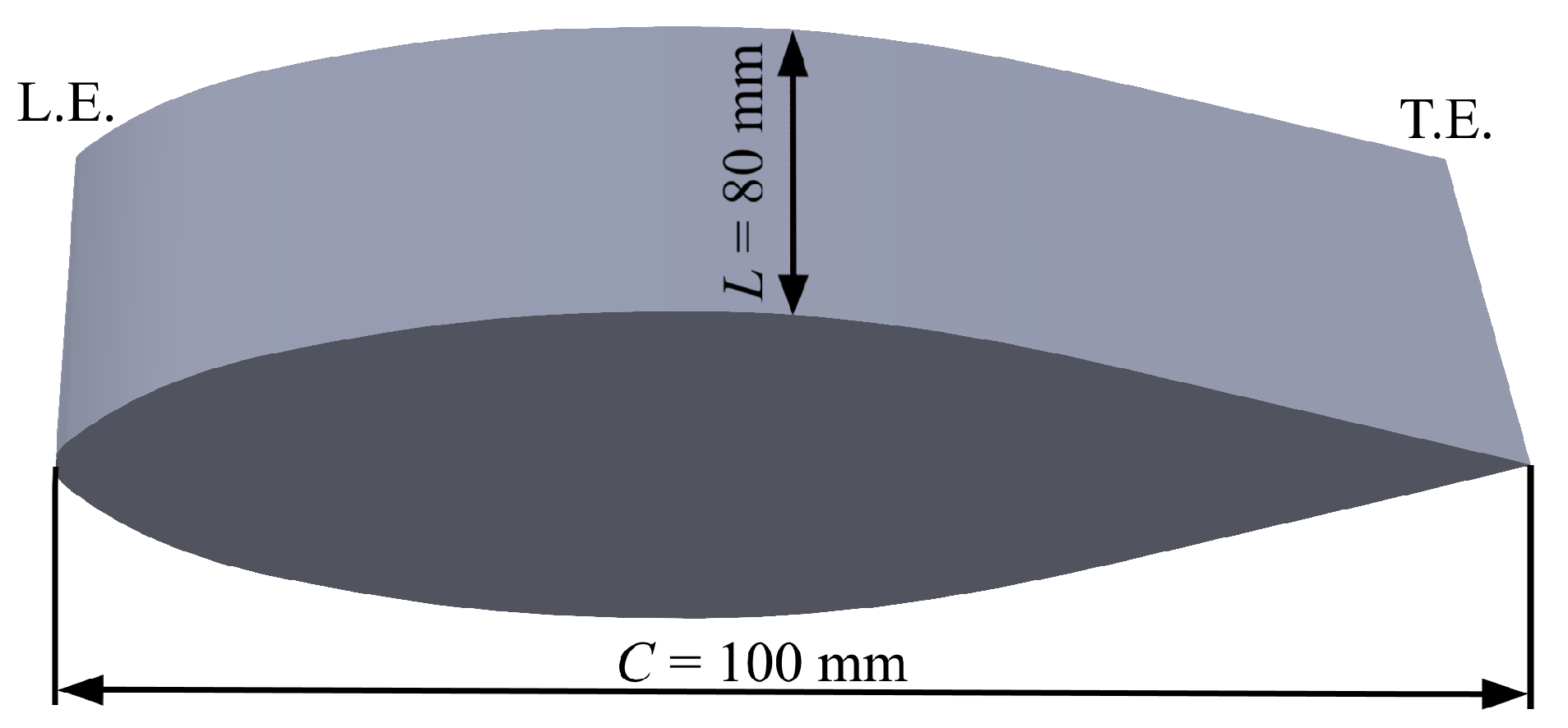
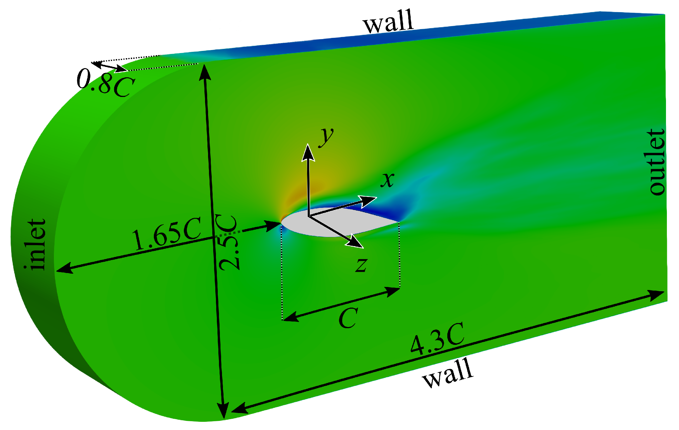
2. Experimental Setup and Flow Regimes

The experimental part of this research was performed in the cavitation tunnel in the Institute of Thermophysics SB RAS described previously [52]. The test section of the tunnel is a 1.3 m long channel with a rectangular cross-section of 0.08 × 0.25 m 2 . We selected a hydrofoil section with a 2D symmetric profile resembling a scaled-down model of guide vanes of a Francis turbine (to a scale of 1:13.26) as a test object, see [53]. The chord length C is 100 mm and the aspect ratio is L / C = 0.8 , where L = 80 mm is the foil span that is equivalent to the width of the test section, see Figure 1. The centerline of the rotating axis of the profile coincides with the geometric center of the hydrofoil. The test model is supported as a cantilever on one of the test channel sidewalls adjoining tightly to both of them, with the distance from the inlet cross-section to the hydrofoil center equal to 7.5 C = 750 mm.
We consider two flow regimes for the attack angle α = 9 ° corresponding to transitional sheet and unsteady cloud cavitation regimes with the flow parameters provided in Table 1. When a cavitation sheet is quasisteady, its closure is almost stable and only minor oscillations of its length are detectable (regime II). In this regime, a vapor trail is often visible alongside the model surface and in the hydrofoil wake due to irregular detachments of tiny vapor clouds from the cavity closure [25,26,54,55]. Unsteady cloud cavitation reveals unstable behavior characterized by quasiperiodic large-scale vapor structures shedding (regime I). In fact, cloud cavitation is one of the most common forms of cavitating flow unsteadiness [5,56,57,58].
The Reynolds and cavitation numbers are defined as
R e C = ρ l U 0 C μ l , σ = p 0 p v ρ l U 0 2 / 2 ,
where p 0 and p v are the reference static pressure at the test section sidewall gauged by a diaphragm strain-gauge pressure transducer near the inlet cross-section at a distance of 7 C = 700 mm upstream from the leading edge of the hydrofoil and the saturation vapor pressure of the operating liquid (distilled water), ρ l and μ l are the density and dynamic viscosity of the operating liquid. Subscripts l and v denote the liquid and vapor phase, respectively. The reference velocity U 0 corresponds to the incoming flow measured upstream of the hydrofoil by PIV in the central vertical longitudinal section over the entire height of the test channel close to the inlet. Both dimensionless quantities ( R e C and σ ) are controlled by changing U 0 . At water temperature of 30 °C, ρ l = 995.61 kg/m 3 , μ l = 7.978 × 10 4 Pa × s and p v = 4.24 × 10 3 Pa. Concentration of the dissolved oxygen in the operating liquid is monitored by a Mettler Toledo InPro 6850i sensor (measurement range from 6 ppb to saturation, relative error 1%) connected to a M400 multiparameter transmitter and maintained almost constant (about 7.4 mg/L) for both flow regimes.
We used a high-speed Photron FASTCAM SA5 camera to visualize the overall cavitating flow and determine integral characteristics of cavitation structures and a PIV method to measure planar velocity distributions around the hydrofoil. Sufficient details on the measurement instrumentation employed for the PIV implementation, processing, and validation procedures to evaluate velocity vector fields and assessment of measurement uncertainties for various statistical characteristics are available in our recent study [59]. The processing routine applied to raw PIV images accounts for local tracer concentration. Velocity vectors are calculated in image areas where seeding particles are suspended corresponding merely to the liquid phase since the vapor phase is free of tracers. This is clearly visible in Figure 2, where velocity vectors are present only in the flow regions without cavitation structures while the regions occupied by the vapor phase do not contain velocity vectors. These measurement data features based only on the liquid phase require an appropriate conditional averaging applied to the numerical results for a consistent and systematic validation as described below.

3. Modeling and Computational Details

In this section, we describe the modeling strategy assuming isothermal flow conditions and neglecting the effects of the surface tension.

3.1. Governing Equations

The Navier–Stokes and VOF equations for a fluid with variable density and viscosity are as follows [51]:
( ρ u i ) t + ( ρ u i u j ) x j = p x i + σ i j x j ,
ρ t + ( ρ u j ) x j = 0 ,
( ρ v α ) t + ( ρ v α u j ) x j = R ,
where
σ i j = μ u i x j + u j x i 2 3 δ i j u k x k
is the viscous stress tensor. The VOF framework determs ρ and μ as follows:
ρ = α ρ v + ( 1 α ) ρ l , μ = α μ v + ( 1 α ) μ l .
Thus, the scalar field α representing the vapor volume fraction varies from 0 for the liquid phase to 1 for the vapor.

3.2. Cavitation Modeling

The term R in Equation (4) is responsible for phase transitions. We employ the Schnerr–Sauer model [16] as a basic approach and compare results to the Kunz model [15]. The Schnerr–Sauer model is formulated in the following way:
R = ρ v ρ l ρ α ( 1 α ) 3 R b sign ( p v p ) 3 2 | p v p | ρ l ,
R b = 3 4 π 1 n 0 α 1 α 1 / 3 .
The only empirical parameter is n 0 corresponding to bubble concentration per a unit volume of liquid and determining the mean radius of a cavitation microbubble which is set to be n 0 = 1.6 × 10 13 according to the original publication [16].
The Kunz model involves more empiricism:
R = C 1 α ρ v 2 min [ p p v , 0 ] ρ l ( 0.5 ρ l U 0 2 ) t 0 + C 2 ( 1 α ) α 2 ρ v t 0 ρ l ,
where t 0 = C / U 0 is the flow characteristic time, and C 1 = C 2 = 1.0 × 10 3 are empirical constants.

3.3. Large-Eddy Simulation Framework

In line with the common routine, we introduce Favre-averaged quantities convenient for variable-density flows [51,60], which are defined as follows:
u ^ i = ρ u i ˜ / ρ ˜ ,
where the tilde denotes local spatial filtering within the LES framework. Applying spatial filtering to Equations (2)–(4) after some manipulations, we arrive at the system of equations:
( ρ ˜ u ^ i ) t + ( ρ ˜ u ^ i u ^ j ) x j = p ˜ x i + σ ^ i j x j τ ^ i j x j ,
ρ ˜ t + ( ρ ˜ u ^ j ) x j = 0 ,
( ρ v α ˜ ) t + ( ρ v α ˜ u ^ j ) x j = R ˜ q ^ j x j ,
where
σ ^ i j = μ ˜ u ^ i x j + u ^ j x i 2 3 δ i j u ^ k x k .
We express the continuity Equation (12) in the form:
u ^ j x j = 1 ρ ˜ d ρ ˜ d t = ρ v ρ l ρ ˜ d α ˜ d t ,
where the substantial derivative and Equation (6) for ρ ˜ were used to obtain this last relation. The subgrid-scale stresses in Equation (11) contain the input from the convective and viscous terms due to the nonlinearity:
τ ^ i j = ρ ˜ u i u j ^ ρ ˜ u ^ i u ^ j + σ ˜ i j σ ^ i j .
A similar term appears in Equation (13):
q ^ j = ρ v α u j ˜ ρ v α ˜ u ^ j .
Below we summarize a list of modeling assumptions:
  • In a standard manner we ignore the commutation errors within the LES framework caused by the inhomogeneous mesh [12].
  • The term τ ^ i j in Equation (11), see Equation (16), is modeled employing a subgrid-scale model without distinguishing between the effects of convective and viscous contributions.
  • We add an additional term ( ρ v α ˜ ( 1 α ˜ ) v ^ j ) / x j to the left-hand-side of Equation (13), where v ^ = u ^ v u ^ l is the relative velocity vector between the two phases, which is also called the compression velocity [61]. It is sometimes described as an artificial term added to compress the interface, but in fact is directly derived from the mass conservation equation of the vapor phase. The compression velocity is modeled as:
    min [ C α | u ^ | , max ( | u ^ | ) ] α ˜ | α ˜ | ,
    which is based on the maximum velocity in some region of the interface, C α = 1 is the constant that controls intensity of the interface compression.
  • The term R ˜ ( α ) in Equation (13) is nonlinear; thus, it has to be modeled. We ignore this fact employing the relation R ˜ ( p , ρ , α ) = R ( p ˜ , ρ ˜ , α ˜ ) .
  • The term q ^ j in Equation (13), see Equation (17), is typically neglected to avoid additional diffusion in the equation for α ˜ .
The subgrid stresses τ ^ i j are approximated using Dynamic k–equation subgrid-scale model (DKSGS) [62]. An additional transport equation is written as follows:
ρ ˜ k s g s t + ρ ˜ u ^ j k s g s x j = ρ τ ^ i j S ^ i j ϵ x j ρ ˜ ( ν + ν t ) k s g s x j ,
where k s g s = u 2 ^ u ^ 2 is the subgrid-scale (SGS) kinetic energy, S ^ i j = ( u ^ i / x j + u ^ j / x i ) / 2 is the strain-rate tensor. The term τ ^ i j is expressed in the following way of the SGS eddy viscosity ν t :
τ ^ i j = 2 ν t S i j ^ + 2 3 δ i j k s g s ,
where ν t = C ν k s g s Δ ˜ and C ν is an unknown coefficient. The dissipation term ϵ is expressed according to the scaling arguments:
ϵ = C ϵ ρ ˜ k s g s 3 / 2 / Δ ˜ ,
where Δ ˜ is the characteristic width of the spatial filter and C ϵ is also an unknown coefficient. The Germano–Lilly [63,64] procedure is applied for the calculations to find the coefficients C ν and C ϵ .

3.4. Numerical Details

LES of the cavitating flow is performed using the computational code OpenFOAM [65] based on the finite volume method (FVM) and interPhaseChangeDyMFoam solver. Within the FVM approach, the computational domain is divided into polyhedral cells with the equations of motion written in the integral form. For the convective term discretization in the momentum equation, see Equation (11), we use two different schemes. The basic one is the second order accurate Linear upwind differencing scheme (LUDS) [47], see the results described in Section 4.4. The results obtained with LUDS are compared to simulations with MUSCL as well as the TVD approach (Total variation diminishing) with MINMOD limiter [49], see Section 4.4. The diffusion terms are discretized using second-order central differences. The van Leer scheme [66] is applied for the second term in Equation (13) to guarantee boundedness of the scalar field. For time discretization we use the Crank–Nicolson scheme [67]. The PISO scheme consisting of a predictor and corrector steps is used for velocity-pressure coupling [68].
The computational domain is shown in Figure 3, where x, y and z correspond to the streamwise, transversal, and spanwise directions, accordingly. An unstructured computational mesh contains around 10.1 × 10 6 nodes. In the simulation, the dynamic mesh refinement procedure [69] is employed leading to an increase in the number of cells to 20 × 10 6 nodes. Dynamic refinement is applied based on the local volume fraction of vapor α by dividing the hexagonal volumes into 8 subvolumes for the cells with 0.4 < α ˜ < 0.6 , see the inset in Figure 4. For detailed information about mesh refinement, the reader is referred to Section 4.1. Nondimensional computational time step Δ t = 1.2 × 10 5 , which corresponds to the CFL number of 0.51 . On the walls we set the no-slip boundary condition. The inflow velocity profile is set in agreement with the experiments [59], while the convective boundary condition is put on the outflow. The inflow boundary conditions for the subgrid-scale kinetic energy k s g s and the volume vapor fraction α ˜ are set to fixed values close to zero. As for the pressure field, the Neumann conditions are specified at all boundaries, while the pressure at the inlet cross-section is extrapolated according to the pressure value p 0 measured upstream. To do that, the velocity field known from the experiment is integrated over the area of the inlet cross-section of the channel. Then, we find the change in pressure along the channel from the cross-section where p 0 is gauged to the inlet cross-section of the computational domain at a distance of 1.65 C from the leading edge of the hydrofoil, Figure 3. The pressure p i n obtained in this way is ultimately set at the inlet cross-section of the computational domain, see Table 1.

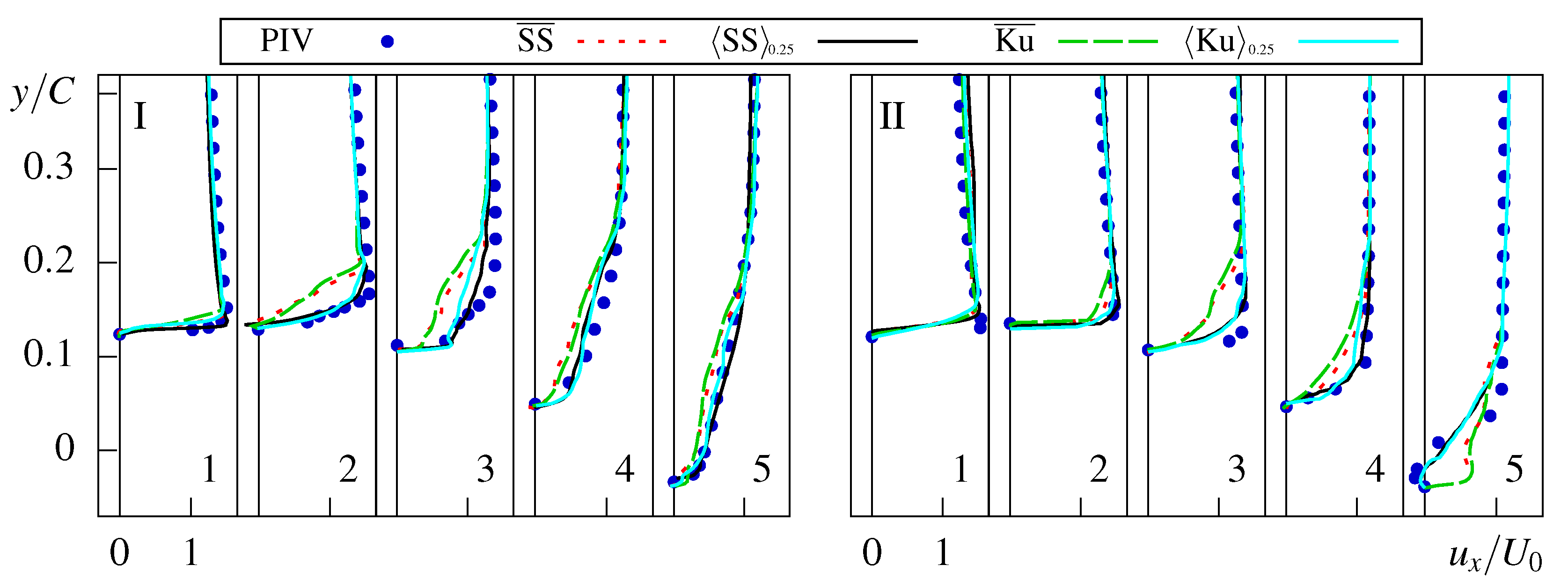
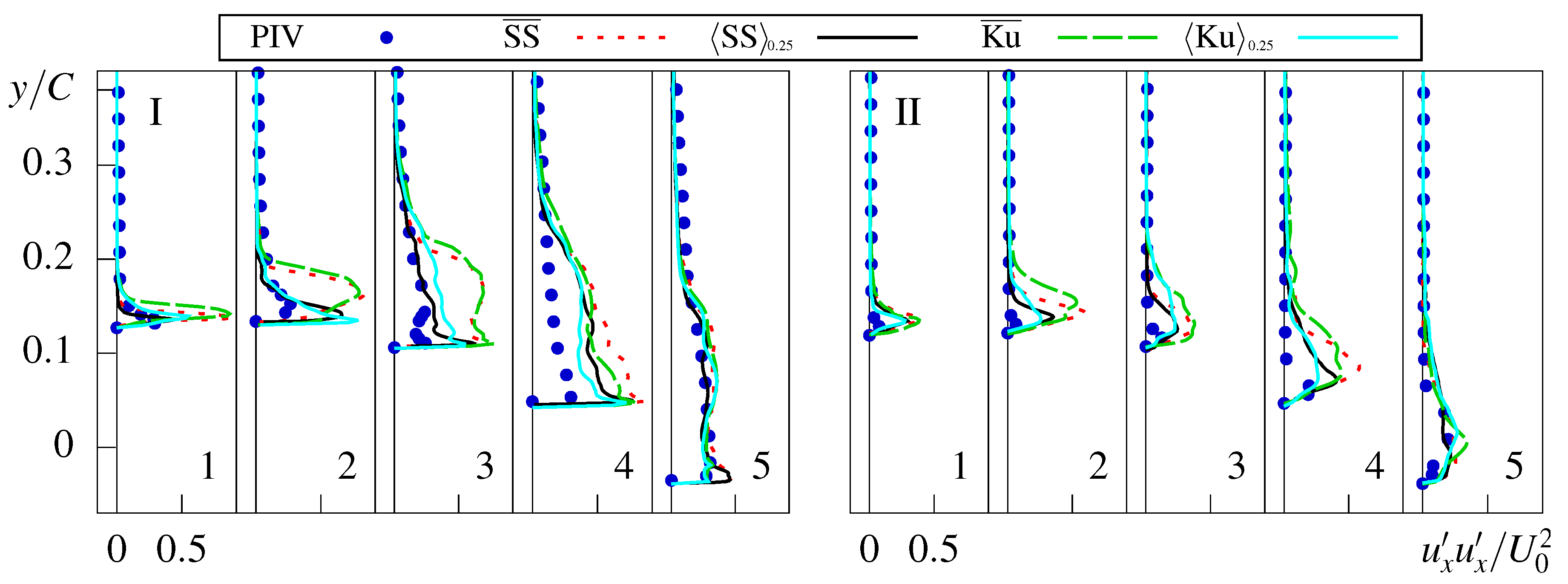
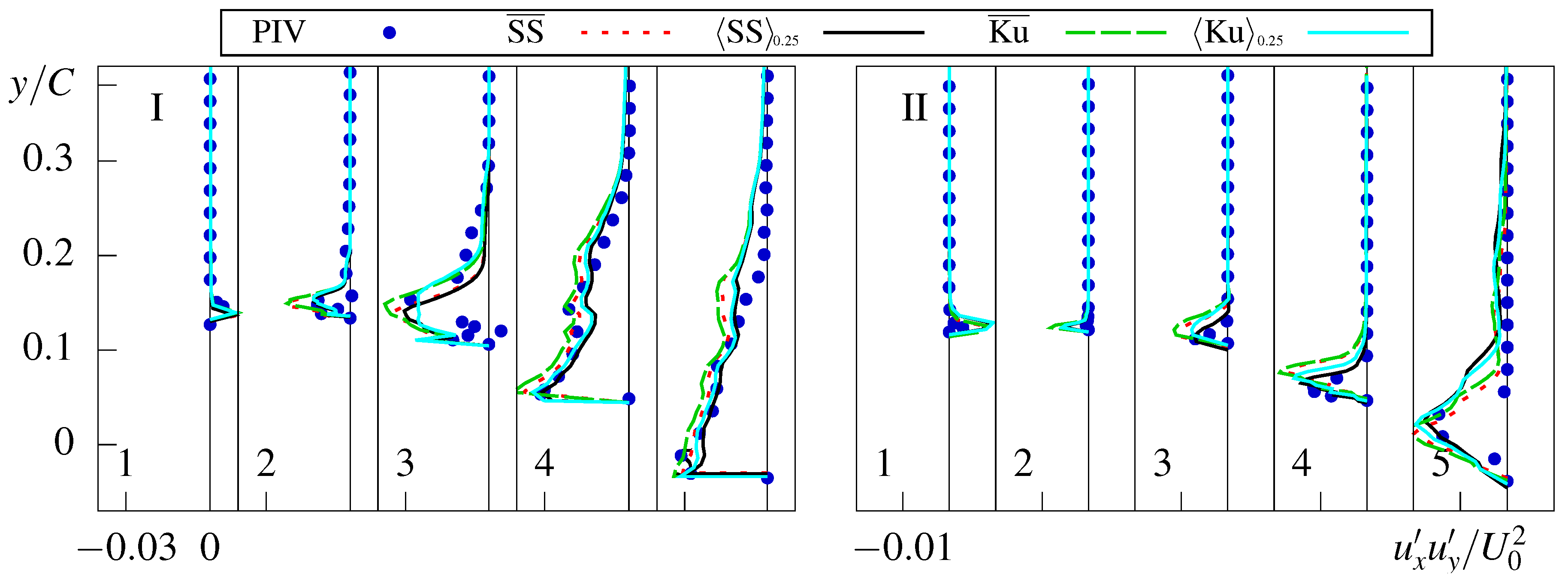
3.5. Conditional Averaging

A reasonable way to adequately compare LES and PIV data for unsteady flow conditions is to perform conditional averaging of velocity fields for certain values of α ˜ to account only for the liquid phase characteristics as in PIV, see Section 2. The conditional averaging of velocity fields is defined as:
u ^ i α ˜ t h = u ^ i | α ˜ < α ˜ t h ,
where averaging . is performed only for samples with α ˜ < α ˜ t h in the same spatial position, where α ˜ t h is a fixed threshold. Obviously, comparison should be performed for real velocity fields rather than for Favre-averaged values. However, the influence of spatial filtering for both LES and PIV appears to be of minor significance as we can see from the direct comparison below.
The value of α ˜ t h was varied in a set of preliminary simulations showing a negligible influence on the results for small vapor fractions, thus, α ˜ t h = 0.25 is adapted. Figure 5 shows the effect of conditional averaging on the mean velocity for regime I. The described procedure makes it possible to obtain the velocity field very close to the experimental one.

4. Results and Discussion

We compare PIV and LES results for the two flow regimes, i.e., regime I ( R e C = 1.32 × 10 6 ) and regime II ( R e C = 1.19 × 10 6 ), see Table 1. The regime with the higher Reynolds number is considered first as it corresponds to unsteady cloud cavitation, which may be more suitable for the chosen LES model. Regime II for transitional sheet cavitation could be expected to be more challenging albeit delivering similarly good results as described below.

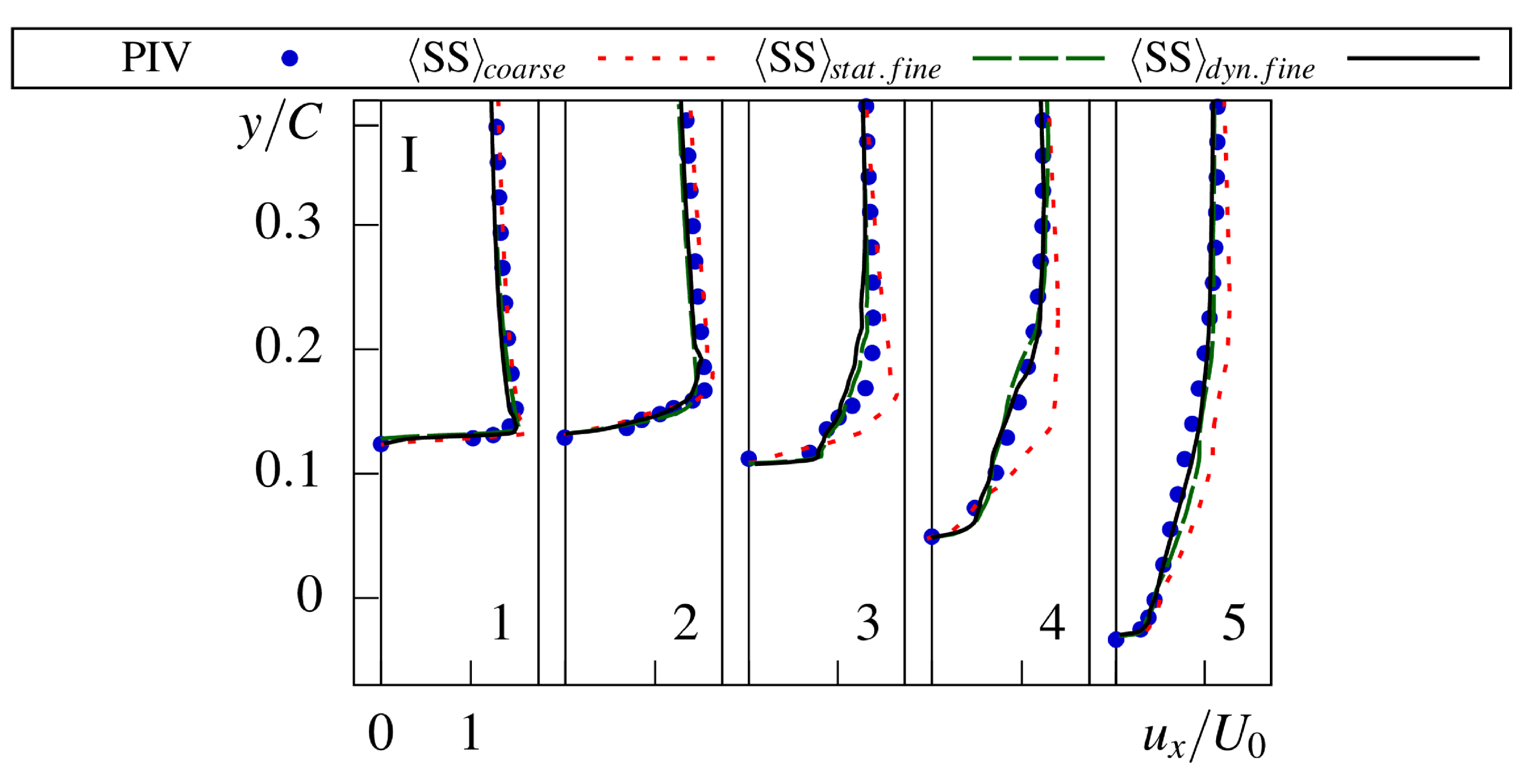
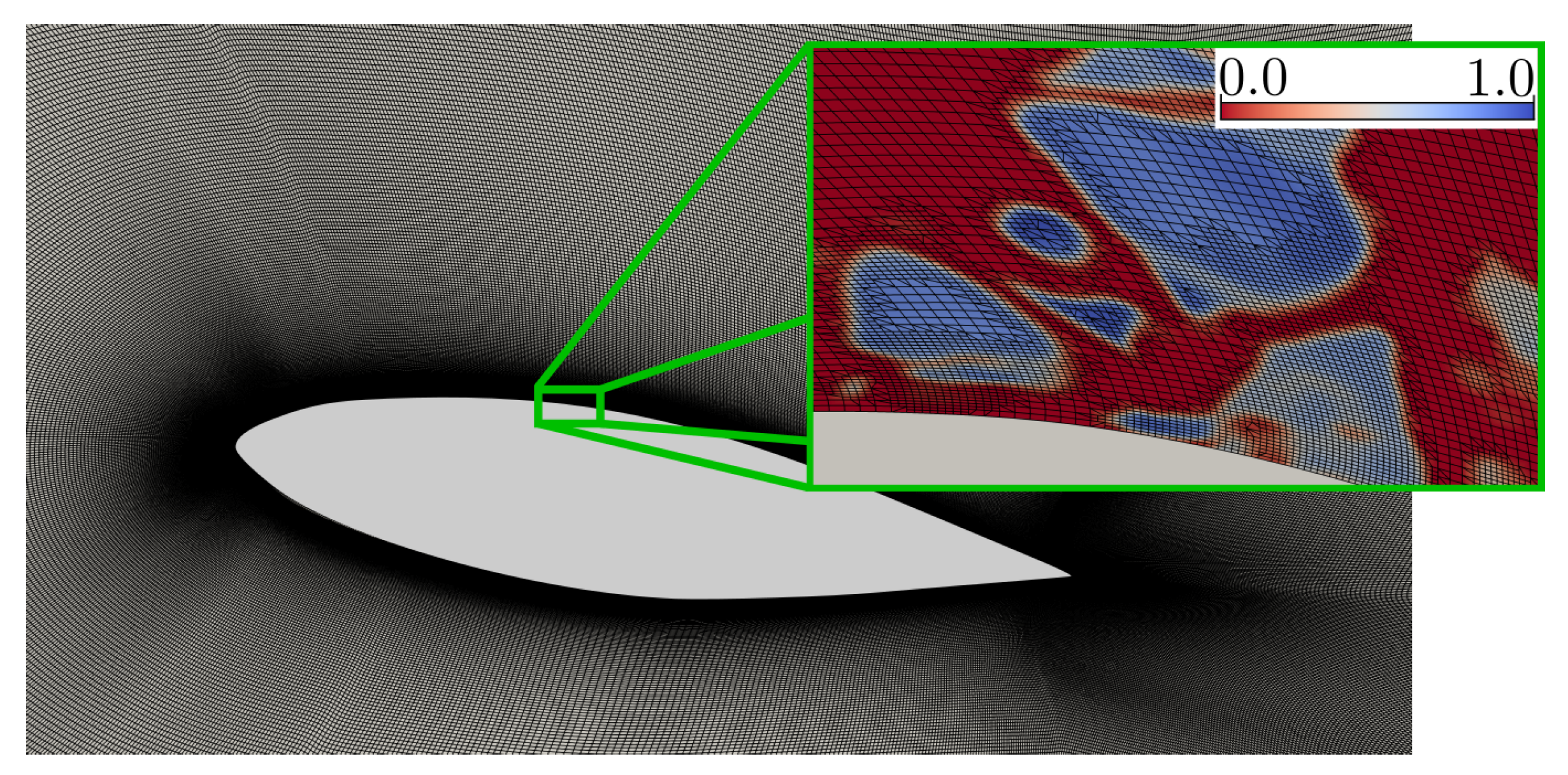
4.1. Mesh Refinement

The dynamic mesh refinement procedure was used to alter the mesh density throughout the domain during the calculation. We considered two cases of the mesh named ‘coarse’ and ‘fine’ to investigate the effect of the mesh refinement on capturing the cavitation structures. As mentioned above, a coarse mesh contained around 10.1 × 10 6 computational nodes. The number of nodes along the upper side of the hydrofoil was 380. In y-direction the number of computational nodes was 430 from the hydrofoil upper side to the upper wall of the domain and the average distance to the first node from the surface was equal to 2.3 × 10 5 C . The dynamic mesh refinement procedure increased a number of nodes along the upper side of the hydrofoil to 620 as well as in y direction to 550 leading to a decrease in the average distance to the first node almost twice. As for a typical large cavitation cloud with the transverse size of around 0.3 C , the number of computational nodes was ∼140 in the y-direction for the coarse mesh, while for the fine mesh it was ∼260. The number of cells increased nearly twice in the region where the cavitation was present. We also considered a mesh with an increased number of computational nodes in the region near the upper side of the hydrofoil. The refined region represented a volume of the size of ( Δ x / C × Δ y / C × Δ z / C ) = (1 × 0.395 × 0.8) built around the center of the foil. In this region, each computational volume was divided into 8 subvolumes leading to 26.5 × 10 6 nodes of computational mesh. The dynamic mesh refinement procedure led to a significant improvement in the accuracy of calculations, see Figure 6, demonstrating the refinement effect on the time-averaged profiles of the streamwise velocity component. Compared to the mesh with the dynamic refinement, the static refinement delivered similar results. Nevertheless, the dynamic refinement was chosen due to the large number of computational nodes for the static refinement.
Figure 7 shows typical moments of the cavity detachment obtained with and without the dynamic mesh refinement procedure and with the static mesh refinement over the upper side of the hydrofoil. Simulations without the refinement perform poorly in capturing the attached vapor clouds because the mesh size appears to be insufficient for a large number of fine structures to be resolved. The patterns of cavitation structures obtained using static refinement and dynamic refinement have no visual differences. However, due to the fact that the mesh with the static refinement has a larger number of computational nodes and consumes more computational resources, the mesh with the dynamic refinement is used in this paper.

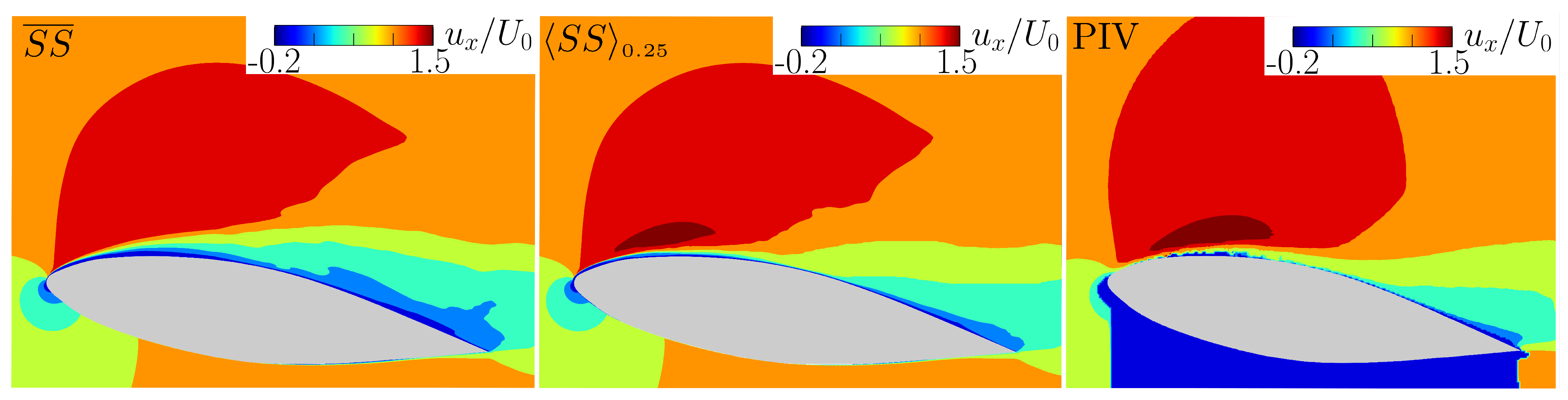
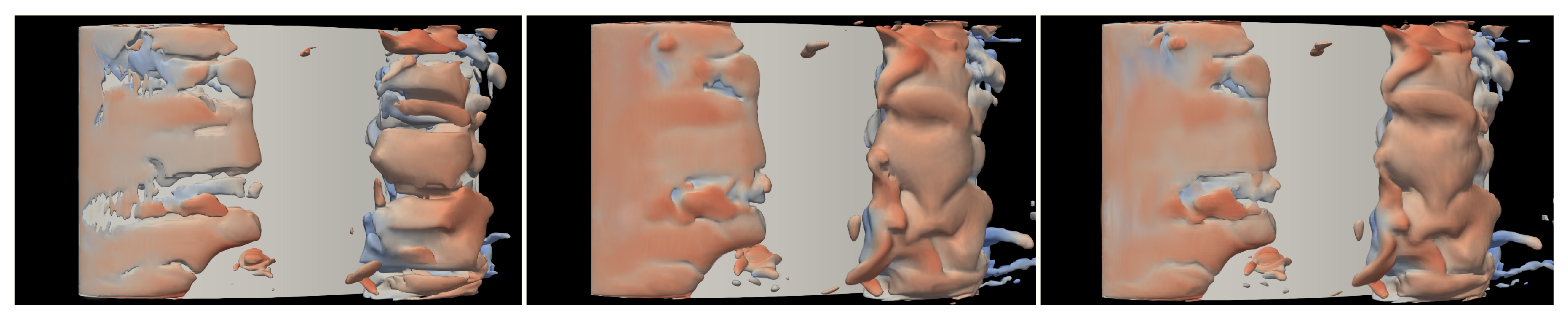
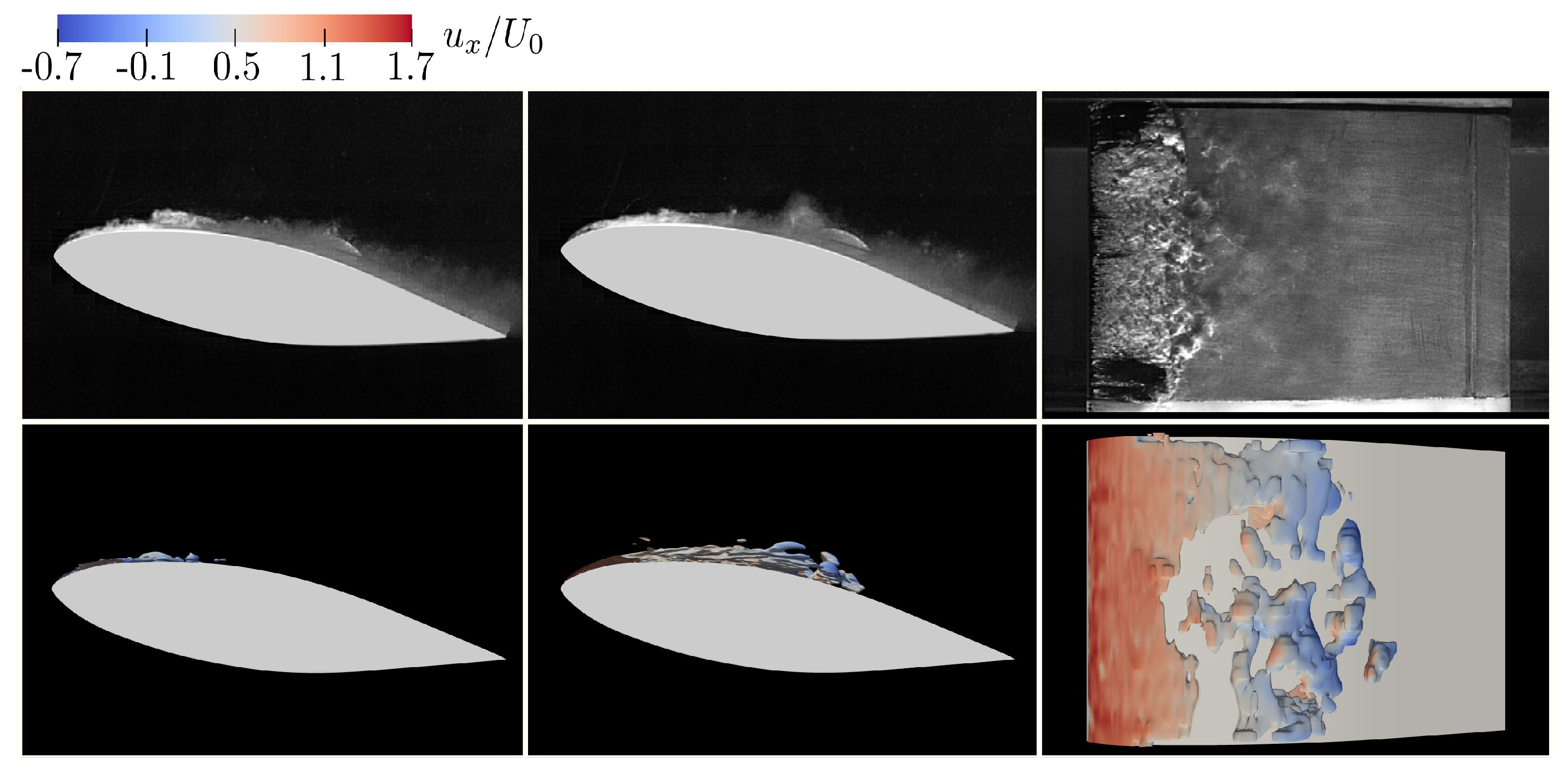
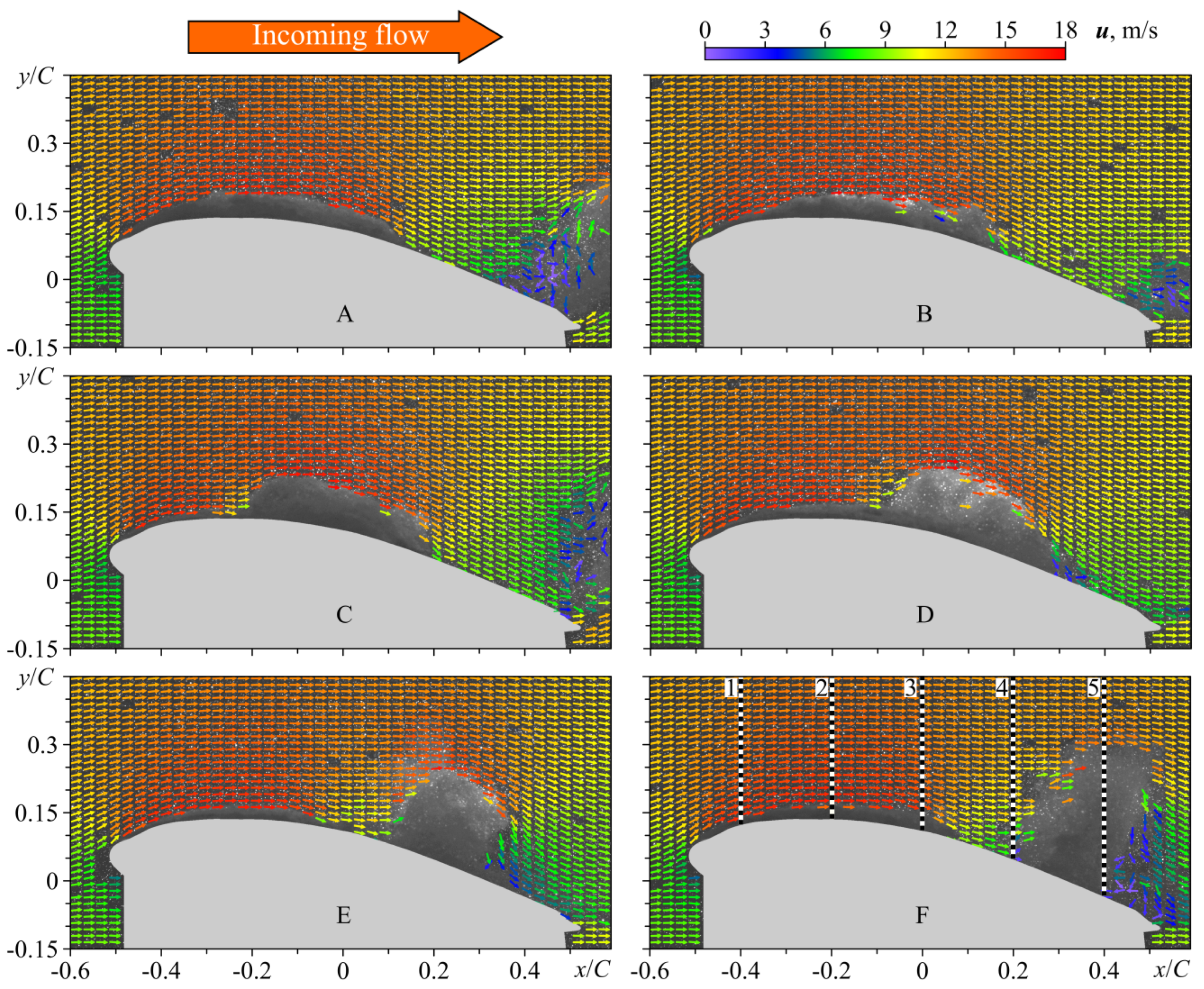
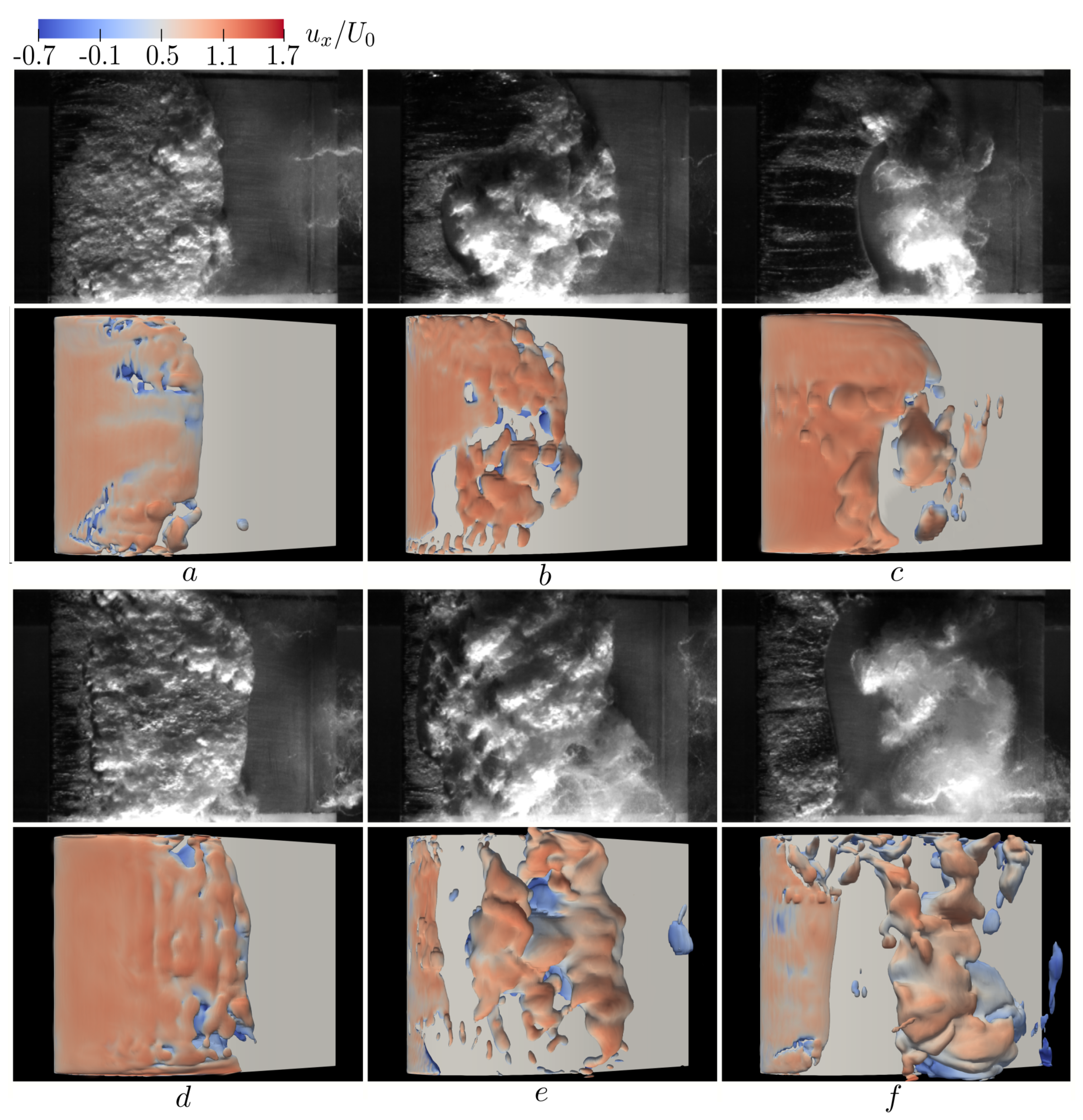
4.2. Visualization and Flow Dynamics

Snapshots during high-speed recording were taken at a sampling rate of 20 kHz, i.e., 20 thousand images correspond to 1 second of real time lapse. This made it possible to directly compare experimental photographs of the cavity with isosurfaces of the instantaneous vapor fraction obtained in the LES calculations. In the simulation, the exposure time of each frame is 1/25,000 of a second. Figure 8 shows a set of photographs of the unsteady cloud cavitating flow together with an isosurface of the instantaneous vapor fraction provided by LES with the Schnerr–Sauer model for regime I. This regime is characterized by a progressive growth of a cavitation sheet followed by its quasiperiodic detachments from the hydrofoil surface, cloud cavity formation, and shedding. This flow unsteadiness is caused by the development of a re-entrant jet moving upstream underneath the attached cavity due to an adverse pressure gradient. According to the cloud size, we distinguish partial, see Figure 8c, and full detachment, see Figure 8f. Immediately after the cloud detachment, the cavity closure front obtains a U-shaped contour. In this case, the attached cavity grows again in the central part of the channel, while close to the sidewalls its length does not change substantially. This behavior is apparently pronounced both in the experiment and simulation, see a–f in Figure 8. The reduced frequency (Strouhal number) of cloud cavitation S t = f C / U 0 , where f is the cavity shedding frequency, is well reproduced by LES with S t L E S 0.20 that is very close to S t P I V 0.19 . The higher dominant frequency S t L E S 0.58 in LES is slightly lower than that in the experiment with S t E x p 0.61 . Such good agreement of the S t values for regime I confirms that the cavitation Schnerr–Sauer model is appropriate and the level of spatial resolution is sufficient for simulating unsteady cloud cavitation.
Contrary to regime I, regime II features quasisteady flow dynamics with uniform detachments of small-scale clouds from the sheet cavity closure in the spanwise direction. Similar to the previous case, Figure 9 shows two characteristic instants for quasi-steady cavitating flow conditions for which some low-amplitude variations in the length of the cavitation sheet are nevertheless observed in the calculations. According to the LES data, there exists a weak quasiperiodicity with the non-dimensional frequency S t L E S 0.23 , although visualization does not reveal any fluctuations of the cavity. This issue still remains unclear and will be addressed in detail in the future. Despite this small discrepancy, the Schnerr–Sauer model visually predicts regime II quite well.

4.3. Comparison of Cavitation Models

To analyze fields of the time-averaged velocity and its fluctuations, we use an improved methodology for a proper comparison of the PIV and LES data based on conditional averaging that accounts only for the liquid phase distinguished by the threshold α ˜ t h = 0.25 , see Equation (21), and then match it against the time-averaged results corresponding to α ˜ t h = 1 . The results are averaged over the total duration of the LES calculations t L E S t o t a l 66 C / U 0 . The PIV measurements were performed with a high spatial resolution, which evidently affects the sampling rate and the total time of the experiment. Each experimental vector corresponds to a window of 8 × 8 pixels or a real flow area of 0.47 × 0.47 mm. PIV data were recorded with a frequency of 4 double frames per second. The high spatial resolution allowed us to make a detailed comparison of the velocity profiles in the selected cross-sections. Values of the mean velocity and its fluctuations were evaluated based on the statistics of 5000 realizations (instantaneous velocity fields), which corresponds to a 20-min series of consecutive measurements in real time or 1255.2 C / U 0 . Figure 10 compares the averaged streamwise velocity profiles for both regimes in the five cross-sections shown in Figure 2, namely x = 0.1 C , 0.3 C , 0.5 C , 0.7 C and 0.9 C . The conditional averaging indeed significantly improves the LES results. Note that the Schnerr–Sauer model typically demonstrates results which are slightly closer to the PIV data in most of the positions compared to the Kunz model. The results for cross-sections 1 and 2 are in excellent agreement, but a small discrepancy is pronounced in positions 3, 4 for regime I and 3, 5 for regime II which is discussed below.
The visual data shown in Figure 8 and Figure 9 demonstrate that, while for regime I the cavitation is basically present in the middle part of the foil, for regime II vapor bubbles are highly concentrated at the trailing edge. This observation explains the discrepancy mentioned above between the PIV and LES results in positions 3, 4 for regime I, and 3, 5 for regime II in Figure 10 representing the most challenging flow regions for modeling as well as the large difference between the time- and conditionally averaged results in these areas. In cross-section 5 for regime I, all the profiles collapse due to intermittent appearances of cloud cavities which periodically pass through this region with a low frequency, leading to a negligible contribution of the vapor phase to the statistical characteristics. Position 5 for regime II demonstrates that the simulation is capable of reproducing a small recirculation zone near the hydrofoil trailing edge, while the time-averaged results point at a relatively high positive velocity due to the vapor phase.
As for the velocity fluctuations averaged conditionally and over the whole time interval, their comparison against the PIV data is shown in Figure 11. Again, it is visible that the conditional averaging significantly improves the LES calculations. The Schnerr–Sauer and Kunz models demonstrate similar results in all cross-sections showing good overall agreement for regime I, except for position 4 where the squared amplitude of the streamwise fluctuations is overpredicted by a factor of 2 compared to the experiments. For cross-sections 2 and 3 of regime I, where the cavitation is largely present, the use of the conditional averaging is essential to reduce the time-averaged value of the velocity fluctuations and match with the experiments. For regime II, the results in the foil midchord, see position 3 in Figure 11, show that LES overestimates the velocity fluctuations compared to PIV, while close to the trailing edge, see position 5, the curves converge for all cases.
As for the conditional averaged shear stress obtained by the Schnerr–Sauer and Kunz models, their profiles are presented in Figure 12 in comparison with the PIV data. For the cross-sections 2 and 3 the conditional averaging reduces the time-averaged value of the shear stress. In positions 4 and 5, the numerical and experimental results are close to each other. The values of the shear stresses for regime II are a bit overestimated but, closer to the trailing edge, they are in good agreement with the PIV measurements. The overall results of the PIV and LES comparison are excellent for most flow regions due to the use of the conditional averaging.

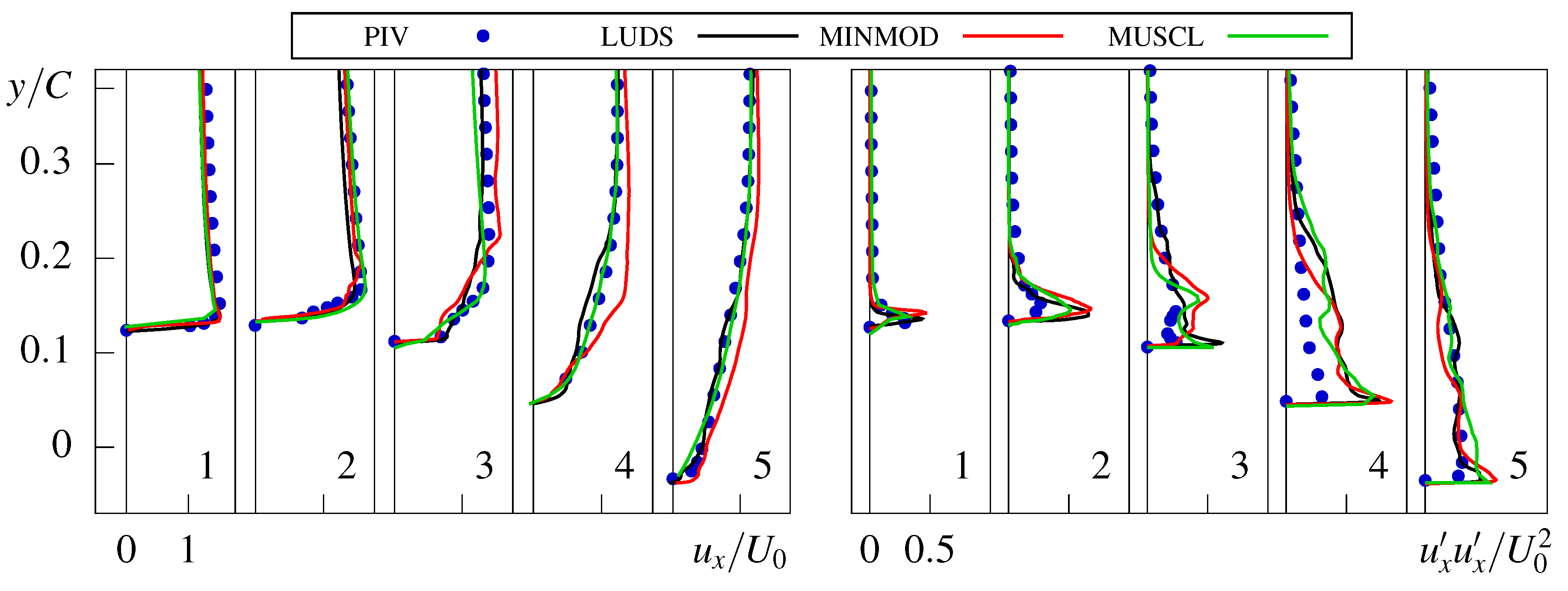
4.4. Comparison of Convective Schemes

Above we compared the two cavitation models using the second-order accurate LUDS scheme to discretize the convective term in the momentum equation, see Equation (11). In this subsection, LUDS is compared with a more dissipative MINMODE and less dissipative MUSCL schemes to highlight the importance of second-order schemes for multiphase LES. Figure 13 shows together profiles of the conditionally averaged velocity and its fluctuations simulated with the Schnerr–Sauer model and the ones measured in the experiment. In the first two cross-sections, slight differences between the curves for LUDS, MINMOD, and MUSCL are clearly seen, which leads to larger deviations downstream. Significant overestimation of the mean velocity in positions 4 and 5 in Figure 13 points out at an enhanced diffusion of the momentum in the spanwise direction for the MINMOD scheme. On the contrary, distributions of the velocity fluctuations exhibit larger deviations in the first three cross-sections, while in positions 4 and 5 they are qualitatively similar. Note that the most delicate near-wall characteristics are poorly predicted by MINMOD, indicating the importance of second-order schemes to describe cavitating flow satisfactorily. The comparison of LUDS and MUSCL showed that there is only a slight discrepancy between these models.

5. Conclusions

We presented results of Large-eddy simulations of transitional sheet and unsteady cloud cavitation flow regimes around a 2D hydrofoil at the angle of attack of 9° and high Reynolds numbers R e C = 1.19 × 10 6 and 1.32 × 10 6 in comparison with the PIV data [53]. We employed finite-volume simulations with the adaptive mesh refinement in critical flow regions where intensive phase transitions occur to increase the overall accuracy together with the Schnerr–Sauer and Kunz cavitation models. The comparison of LES and visualization results confirmed that the flow dynamics in the unsteady cloud cavitation regime was correctly reproduced in the numerical simulations including the shedding frequencies of partial and full detachment of cloud cavities and typical U-shaped front of the cavitation sheet closure after the cavity breakup.
To compare averaged velocity fields, we take into account that the measured PIV data provided the information only for the liquid phase. Thus, we proposed a methodology based on the conditional averaging of instantaneous velocity fields including only relatively small vapor fractions. This approach led to excellent overall agreement of distributions of the conditionally averaged velocity over the leading edge of the hydrofoil for both flow conditions. A slight difference between the LES and PIV data for the unsteady cloud cavity regime was observed in the midchord region above the hydrofoil, where the cavitation was very intensive. For the transitional sheet cavitation regime, we observed some discrepancies near the trailing edge of the hydrofoil where the cavitation modeling is quite challenging. The profiles of velocity fluctuations and the main component of shear stresses averaged conditionally over the whole time interval showed that the proposed methodology significantly improves the LES results compared to the PIV data. Next, the importance of the second-order LUDS discretization schemes was highlighted in comparison with corresponding results for the lower-order TVD MINMOD scheme. The comparison of LUDS and MUSCL schemes showed a slight discrepancy. Nevertheless, the results obtained with the LUDS model are in a good agreement with PIV.
Further application of the verified models will allow to study dynamic characteristics of the cavitating flow in more detail with a particular attention to lower-Reynolds-number transitional regimes typically representing a challenge for the considered cavitation models.

Author Contributions

R.M. and K.P. conceived the research; E.I., M.H. and R.M. performed numerical simulations; K.P. and M.T. conducted the experimental part; E.I., K.P. and R.M. wrote the manuscript. All authors have read and agreed to the published version of the manuscript.

Funding

The work was funded by the Ministry of Science and Higher Education of the Russian Federation (Project No. 075-15-2019-1923). The numerical tools as well as the methods of automatization of data acquisition and processing used in the study were developed under a state contract with IT SB RAS.

Institutional Review Board Statement

Not applicable.

Informed Consent Statement

Not applicable.

Data Availability Statement

The data underlying this study are available upon request.

Acknowledgments

The computational resources were provided by the “Cascade” Joint Supercomputer Center of the Institute of Thermophysics and Novosibirsk State University as well as the Joint Supercomputer Center of the Russian Academy of Sciences (Moscow).

Conflicts of Interest

The authors declare no conflict of interest.

References

  1. Plesset, M. Bubble dynamics and cavitation. Annu. Rev. Fluid Mech. 1977, 9, 145–185. [Google Scholar] [CrossRef]
  2. Arndt, R. Cavitation in fluid machinery and hydraulic structures. Annu. Rev. Fluid Mech. 1981, 13, 273–328. [Google Scholar] [CrossRef]
  3. Arndt, R. Cavitation in vortical flows. Annu. Rev. Fluid Mech. 2002, 34, 143–175. [Google Scholar] [CrossRef]
  4. Brennen, C. Cavitation and Bubble Dynamics; Cambridge University Press: Cambridge, UK, 2014. [Google Scholar]
  5. Franc, J.; Michel, J. Fundamentals of Cavitation; Springer Science & Business Media: Berlin/Heidelberg, Germany, 2006. [Google Scholar]
  6. Li, C.; Ceccio, S. Interaction of single travelling bubbles with the boundary layer and attached cavitation. J. Fluid Mech. 1996, 322, 329–353. [Google Scholar] [CrossRef]
  7. Lindau, O.; Lauterborn, W. Cinematographic observation of the collapse and rebound of a laser-produced cavitation bubble near a wall. J. Fluid Mech. 2003, 479, 327–348. [Google Scholar] [CrossRef]
  8. Ausoni, P.; Zobeiri, A.; Avellan, F.; Farhat, M. The effects of a tripped turbulent boundary layer on vortex shedding from a blunt trailing edge hydrofoil. J. Fluids Eng. 2012, 134, 051207. [Google Scholar] [CrossRef]
  9. Gopalan, S.; Katz, J. Flow structure and modeling issues in the closure region of attached cavitation. Phys. Fluids 2000, 12, 895–911. [Google Scholar] [CrossRef]
  10. Huang, B.; Young, Y.; Wang, G.; Shyy, W. Combined experimental and computational investigation of unsteady structure of sheet/cloud cavitation. J. Fluids Eng. 2013, 135, 071301. [Google Scholar] [CrossRef]
  11. Pope, S. Turbulent Flows; Cambridge University Press: Cambridge, UK, 2001. [Google Scholar]
  12. Sagaut, P. Large Eddy Simulation for Incompressible Flows: An Introduction; Springer Science & Business Media: Berlin/Heidelberg, Germany, 2006. [Google Scholar]
  13. Kubota, A.; Kato, H.; Yamaguchi, H. A new modelling of cavitating flows: A numerical study of unsteady cavitation on a hydrofoil section. J. Fluid Mech. 1992, 240, 59–96. [Google Scholar] [CrossRef]
  14. Merkle, C.; Feng, J.; Buelow, P. Computational modeling of the dynamics of sheet cavitation. In Proceedings of the Third International Symposium on Cavitation, Grenoble, France, 7–10 April 1998. [Google Scholar]
  15. Kunz, R.; Boger, D.; Stinebring, D.; Chyczewski, T.; Lindau, J.; Gibeling, H.; Venkateswaran, S.; Govindan, T. A preconditioned Navier–Stokes method for two-phase flows with application to cavitation prediction. Comput. Fluids 2000, 29, 849–875. [Google Scholar] [CrossRef]
  16. Schnerr, G.; Sauer, J. Physical and numerical modeling of unsteady cavitation dynamics. In Proceedings of the Fourth International Conference on Multiphase Flow, New Orleans, LA, USA, 27 May–1 June 2001. [Google Scholar]
  17. Singhal, A.; Athavale, M.; Li, H.; Jiang, Y. Mathematical basis and validation of the full cavitation model. J. Fluids Eng. 2002, 124, 617–624. [Google Scholar] [CrossRef]
  18. Frobenius, M.; Schilling, R.; Bachert, R.; Stoffel, B.; Ludwig, G. Three-dimensional, unsteady cavitation effects on a single hydrofoil and in a radial pump–measurements and numerical simulations, Part two: Numerical simulation. In Proceedings of the Fifth International Symposium on Cavitation, Osaka, Japan, 1–4 November 2003. [Google Scholar]
  19. Coutier-Delgosha, O.; Reboud, J.; Delannoy, Y. Numerical simulation of the unsteady behaviour of cavitating flows. Int. J. Numer. Methods Fluids 2003, 42, 527–548. [Google Scholar]
  20. Saito, Y.; Nakamori, I.; Ikohagi, T. Numerical analysis of unsteady vaporous cavitating flow around a hydrofoil. In Proceedings of the Fifth International Symposium on Cavitation, Osaka, Japan, 1–4 November 2003. [Google Scholar]
  21. Zwart, P.; Gerber, A.; Belamri, T. A two-phase flow model for predicting cavitation dynamics. In Proceedings of the Fifth International Conference on Multiphase Flow, Yokohama, Japan, 30 May–4 June 2004. [Google Scholar]
  22. Senocak, I.; Shyy, W. Interfacial dynamics-based modelling of turbulent cavitating flows, Part-1: Model development and steady-state computations. Int. J. Numer. Methods Fluids 2004, 44, 975–995. [Google Scholar] [CrossRef]
  23. Senocak, I.; Shyy, W. Interfacial dynamics-based modelling of turbulent cavitating flows, Part-2: Time-dependent computations. Int. J. Numer. Methods Fluids 2004, 44, 997–1016. [Google Scholar] [CrossRef]
  24. Owis, F.; Nayfeh, A. Numerical simulation of 3-D incompressible, multi-phase flows over cavitating projectiles. Eur. J. Mech.-B/Fluids 2004, 23, 339–351. [Google Scholar] [CrossRef]
  25. Leroux, J.; Coutier-Delgosha, O.; Astolfi, J. A joint experimental and numerical study of mechanisms associated to instability of partial cavitation on two-dimensional hydrofoil. Phys. Fluids 2005, 17, 052101. [Google Scholar] [CrossRef] [Green Version]
  26. Coutier-Delgosha, O.; Stutz, B.; Vabre, A.; Legoupil, S. Analysis of cavitating flow structure by experimental and numerical investigations. J. Fluid Mech. 2007, 578, 171–222. [Google Scholar] [CrossRef] [Green Version]
  27. Frikha, S.; Coutier-Delgosha, O.; Astolfi, J. Influence of the cavitation model on the simulation of cloud cavitation on 2D foil section. Int. J. Rotating Mach. 2008, 2008, 146234. [Google Scholar] [CrossRef] [Green Version]
  28. Morgut, M.; Nobile, E.; Bilus, I. Comparison of mass transfer models for the numerical prediction of sheet cavitation around a hydrofoil. Int. J. Multiph. Flow 2011, 37, 620–626. [Google Scholar] [CrossRef]
  29. Yang, J.; Zhou, L.; Wang, Z. Numerical simulation of three-dimensional cavitation around a hydrofoil. J. Fluids Eng. 2011, 133, 081301. [Google Scholar] [CrossRef]
  30. Ducoin, A.; Huang, B.; Young, Y. Numerical modeling of unsteady cavitating flows around a stationary hydrofoil. Int. J. Rotating Mach. 2012, 2012, 215678. [Google Scholar] [CrossRef] [Green Version]
  31. Cheng, H.; Bai, X.; Long, X.; Ji, B.; Peng, X.; Farhat, M. Large eddy simulation of the tip-leakage cavitating flow with an insight on how cavitation influences vorticity and turbulence. Appl. Math. Model. 2020, 77, 788–809. [Google Scholar] [CrossRef]
  32. Long, Y.; Long, X.; Ji, B.; Xing, T. Verification and validation of Large Eddy Simulation of attached cavitating flow around a Clark-Y hydrofoil. Int. J. Multiph. Flow 2019, 115, 93–107. [Google Scholar] [CrossRef]
  33. Wang, G.; Ostoja-Starzewski, M. Large eddy simulation of a sheet/cloud cavitation on a NACA0015 hydrofoil. Appl. Math. Model. 2007, 31, 417–447. [Google Scholar] [CrossRef]
  34. Luo, X.; Ji, B.; Peng, X.; Xu, H.; Nishi, M. Numerical simulation of cavity shedding from a three-dimensional twisted hydrofoil and induced pressure fluctuation by large-eddy simulation. J. Fluids Eng. 2012, 134, 041202. [Google Scholar] [CrossRef]
  35. Ji, B.; Luo, X.; Arndt, R.; Peng, X.; Wu, Y. Large eddy simulation and theoretical investigations of the transient cavitating vortical flow structure around a NACA66 hydrofoil. Int. J. Multiph. Flow 2015, 68, 121–134. [Google Scholar] [CrossRef] [Green Version]
  36. Li, L.; Li, B.; Hu, Z.; Lin, Y.; Cheung, S. Large eddy simulation of unsteady shedding behavior in cavitating flows with time-average validation. Ocean. Eng. 2016, 125, 1–11. [Google Scholar] [CrossRef]
  37. Liu, M.; Tan, L.; Cao, S. Cavitation-vortex-turbulence interaction and one-dimensional model prediction of pressure for hydrofoil ALE15 by large eddy simulation. J. Fluids Eng. 2016, 141, 021103. [Google Scholar] [CrossRef]
  38. Gnanaskandan, A.; Mahesh, K. Numerical investigation of near-wake characteristics of cavitating flow over a circular cylinder. J. Fluid Mech. 2016, 790, 453–491. [Google Scholar] [CrossRef] [Green Version]
  39. Brandao, F.; Bhatt, M.; Mahesh, K. Numerical study of cavitation regimes in flow over a circular cylinder. J. Fluid Mech. 2020, 885, A19. [Google Scholar] [CrossRef] [Green Version]
  40. Bensow, R.; Bark, G. Implicit LES predictions of the cavitating flow on a propeller. J. Fluids Eng. 2010, 132, 041302. [Google Scholar] [CrossRef]
  41. Dittakavi, N.; Chunekar, A.; Frankel, S. Large eddy simulation of turbulent-cavitation interactions in a Venturi nozzle. J. Fluids Eng. 2010, 132, 121301. [Google Scholar] [CrossRef]
  42. Zhang, L.; Khoo, B. Computations of partial and super cavitating flows using implicit pressure-based algorithm (IPA). Comput. Fluids 2013, 73, 1–9. [Google Scholar] [CrossRef]
  43. Yu, X.; Huang, C.; Du, T.; Liao, L.; Wu, X.; Zheng, Z.; Wang, Y. Study of characteristics of cloud cavity around axisymmetric projectile by large eddy simulation. J. Fluids Eng. 2014, 136, 051303. [Google Scholar] [CrossRef] [Green Version]
  44. Orley, F.; Trummler, T.; Hickel, S.; Mihatsch, M.; Schmidt, S.; Adams, N. Large-eddy simulation of cavitating nozzle flow and primary jet break-up. Phys. Fluids 2015, 27, 086101. [Google Scholar] [CrossRef] [Green Version]
  45. Gnanaskandan, A.; Mahesh, K. Large eddy simulation of the transition from sheet to cloud cavitation over a wedge. Int. J. Multiph. Flow 2016, 83, 86–102. [Google Scholar] [CrossRef] [Green Version]
  46. Bhatt, M.; Mahesh, K. Numerical investigation of partial cavitation regimes over a wedge using large eddy simulation. Int. J. Multiph. Flow 2020, 122, 103155. [Google Scholar] [CrossRef]
  47. Warming, R.; Beam, R. Upwind second-order difference schemes and applications in aerodynamic flows. AIAA J. 1976, 14, 1241–1249. [Google Scholar] [CrossRef]
  48. Jasak, H. Error Analysis and Estimation for the Finite Volume Method with Applications to Fluid Flows. Ph.D. Thesis, University of Cambridge, Cambridge, UK, 1996. [Google Scholar]
  49. Harten, A. High resolution schemes for hyperbolic conservation laws. J. Comput. Phys. 1997, 135, 260–278. [Google Scholar] [CrossRef] [Green Version]
  50. Ferziger, J.; Perić, M.; Street, R. Computational Methods for Fluid Dynamics; Springer: Berlin/Heidelberg, Germany, 2002; Volume 3. [Google Scholar]
  51. Sagaut, P.; Adams, N.; Garnier, E. Large-Eddy Simulation for Compressible Flows; Springer: Berlin/Heidelberg, Germany, 2009; Volume 276. [Google Scholar]
  52. Kravtsova, A.; Markovich, D.; Pervunin, K.; Timoshevskiy, M.; Hanjalić, K. High-speed visualization and PIV measurements of cavitating flows around a semi-circular leading-edge flat plate and NACA0015 hydrofoil. Int. J. Multiph. Flow 2014, 60, 119–134. [Google Scholar] [CrossRef]
  53. Kravtsova, A.; Pervunin, K.; Timoshevskiy, M.; Churkin, S.; Markovich, D.; Hanjalić, K. Cavitating flow around a scaled-down model of guide vanes of a high-pressure turbine. Int. J. Multiph. Flow 2016, 78, 75–87. [Google Scholar]
  54. Arndt, R.; Song, C.; Kjeldsen, M.; He, J.; Keller, A. Instability of Partial Cavitation: A Numerical/Experimental Approach; National Academies Press: Washington, DC, USA, 2000. [Google Scholar]
  55. Huang, B.; Zhao, Y.; Wang, G. Large eddy simulation of turbulent vortex-cavitation interactions in transient sheet/cloud cavitating flows. Comput. Fluids 2014, 92, 113–124. [Google Scholar] [CrossRef]
  56. Decaix, J.; Goncalves, E. Investigation of three-dimensional effects on a cavitating venturi flow. Int. J. Heat Fluid Flow 2013, 44, 576–595. [Google Scholar] [CrossRef] [Green Version]
  57. Zhang, X.; Zhang, W.; Chen, J.; Qiu, L.; Sun, D. Validation of dynamic cavitation model for unsteady cavitating flow on NACA66. Sci. China Technol. Sci. 2014, 57, 819–827. [Google Scholar] [CrossRef]
  58. Wu, Q.; Huang, B.; Wang, G.; Gao, Y. Experimental and numerical investigation of hydroelastic response of a flexible hydrofoil in cavitating flow. Int. J. Multiph. Flow 2015, 74, 19–33. [Google Scholar] [CrossRef]
  59. Timoshevskiy, M.; Ilyushin, B.; Pervunin, K. Statistical structure of the velocity field in cavitating flow around a 2D hydrofoil. Int. J. Heat Fluid Flow 2020, 85, 108646. [Google Scholar] [CrossRef]
  60. Arabnejad, M.; Amini, A.; Farhat, M.; Bensow, R. Numerical and experimental investigation of shedding mechanisms from leading-edge cavitation. Int. J. Multiph. Flow 2019, 119, 123–143. [Google Scholar] [CrossRef]
  61. Berberović, E.; van Hinsberg, N.; Jakirlić, S.; Roisman, I.; Tropea, C. Drop impact onto a liquid layer of finite thickness: Dynamics of the cavity evolution. Phys. Rev. E 2009, 79, 036306. [Google Scholar] [CrossRef]
  62. Yoshizawa, A.; Horiuti, K. A statistically-derived subgrid-scale kinetic energy model for the large-eddy simulation of turbulent flows. J. Phys. Soc. Jpn. 1985, 54, 2834–2839. [Google Scholar] [CrossRef]
  63. Germano, M.; Piomelli, U.; Moin, P.; Cabot, W. A dynamic subgrid-scale eddy viscosity model. Phys. Fluids Fluid Dyn. 1991, 3, 1760–1765. [Google Scholar] [CrossRef] [Green Version]
  64. Lilly, D. A proposed modification of the Germano subgrid-scale closure method. Phys. Fluids A Fluid Dyn. 1992, 4, 633–635. [Google Scholar] [CrossRef]
  65. OpenFOAM. Project Site. 2004. Available online: http://www.openfoam.com (accessed on 20 October 2021).
  66. Van Leer, B. Towards the ultimate conservative difference scheme. II. Monotonicity and conservation combined in a second-order scheme. J. Comput. Phys. 1974, 14, 361–370. [Google Scholar] [CrossRef]
  67. Crank, J.; Nicolson, P. A practical method for numerical evaluation of solutions of partial differential equations of the heat-conduction type. In Mathematical Proceedings of the Cambridge Philosophical Society; Cambridge University Press: Cambridge, UK, 1947; Volume 43, pp. 50–67. [Google Scholar]
  68. Moukalled, F.; Mangani, L.; Darwish, M. The Finite Volume Method in Computational Fluid Dynamics; Springer: Berlin/Heidelberg, Germany, 2016; Volume 113. [Google Scholar]
  69. OpenFOAM. Dynamic Mesh Refine Library. 2019. Available online: https://holzmann-cfd.com/community/training-cases/adaptive-mesh-refinement (accessed on 20 October 2021).
Figure 1. 3D model of hydrofoil section. L.E. and T.E. stand for leading and trailing edges of hydrofoil, respectively.
Jmse 09 01193 g001
Figure 2. Instantaneous velocity vector fields around hydrofoil at different phases of oscillation period (AF) for unsteady cloud cavitation conditions (regime I). Every sixth and every third vector is shown in vertical and horizontal direction, respectively. Gray mask covers the image area occupied by hydrofoil and its shadow below. Dashed black-white vertical lines in image F denote cross-sections in which profiles of various turbulence quantities are presented below.
Jmse 09 01193 g002
Figure 3. Overall view of computational domain, boundary conditions, and coordinate system.
Jmse 09 01193 g003
Figure 4. Computational mesh around hydrofoil in the x y plane. Blow-up shows an instantaneous vapor field α ˜ to demonstrate dynamic mesh refinement procedure.
Jmse 09 01193 g004
Figure 5. Comparison of experimental and numerical fields of the streamwise component of the time-averaged velocity for regime I in longitudinal midspan section of hydrofoil. Results of the Schnerr-Sauer (SS) model with LUDS discretization scheme for convective term in momentum equation are presented for time-averaging ( . ) ¯ and conditional averaging . α ˜ t h procedures according to Equation (21). The threshold value of α ˜ t h is chosen equal to 0.25 .
Jmse 09 01193 g005
Figure 6. Comparison of experimental and numerical profiles of the streamwise component of averaged velocity for regime I. Results of Schnerr–Sauer (SS) model are presented for conditional averaging procedure with threshold value of α ˜ t h = 0.25 together for coarse, mesh with dynamic refinement, and mesh with static refinement.
Jmse 09 01193 g006
Figure 7. Comparison of patterns of cavitation structures in regime I for coarse (left), dynamic refinement (middle), and static refinement (right) meshes: isosurface α ˜ = 0.5 colored with streamwise velocity u x from LES using Schnerr–Sauer model.
Jmse 09 01193 g007
Figure 8. Comparison of cavitation structures at six characteristic time instants (af) colored with the streamwise velocity u x for regime I: snapshots captured in experiment (top row) and isosurface α ˜ = 0.5 from LES using Schnerr-Sauer model and LUDS discretization scheme (bottom row). Right column is a top view of the same cavitation patterns shown in the middle images.
Jmse 09 01193 g008
Figure 9. Similar to Figure 8 for regime II.
Jmse 09 01193 g009
Figure 10. Comparison of experimental and numerical profiles of streamwise component of averaged velocity for regime I (left) and II (right) in cross-sections depicted in Figure 2 at hydrofoil midspan. Results of Schnerr–Sauer (SS) and Kunz (Ku) models with LUDS discretization scheme for convective term in momentum equation are both presented for time-averaging ( . ) ¯ and conditional averaging . α ˜ t h procedures according to Equation (21). The threshold value of α ˜ t h is chosen to be equal to 0.25 .
Jmse 09 01193 g010
Figure 11. Similar to Figure 10 for streamwise velocity fluctuations.
Jmse 09 01193 g011
Figure 12. Similar to Figure 10 for the main component of shear stresses.
Jmse 09 01193 g012
Figure 13. Comparison of experimental and numerical profiles of the streamwise component of conditionally averaged velocity and its fluctuations for regime I with α ˜ t h = 0.25 based on Schnerr–Sauer model.
Jmse 09 01193 g013
Table 1. Flow regimes considered in present study.
U 0 [m/s] p 0 [kPa] p i n [kPa] R e C [-] σ [-]
I 10.47 105.8 85.3 1.32 × 10 6 1.86
II 9.45 115.3 102.4 1.19 × 10 6 2.49
Publisher’s Note: MDPI stays neutral with regard to jurisdictional claims in published maps and institutional affiliations.

