Numerical Simulation of Cavitation and Damping Force Characteristics for a High-Speed Supercavitation Vehicle

Abstract

In this study, an attempt has been made to investigate the supercavitation and hydrodynamic characteristics of high-speed vehicles. A homogeneous equilibrium flow model and a Schnerr–Sauer model based on the Reynolds-averaged Navier–Stokes method are used. Grid-independent inspection and comparison with experimental data in the literature have been carried out to verify the accuracy of numerical methods. The effect of the navigation speed and angle of attack on the cavitation morphology and dynamic characteristics has been investigated. It has been demonstrated that the angle of attack has a remarkable influence on the wet surface and hydrodynamic force, whereas navigation speed has little effect on the position force of the vehicle under the circumstance of no wet surface. The hydrodynamic force changes periodically with the swing of the vehicle, but its maximum is greater than that for the direct navigation state at the same attack angle. Moreover, the damping effect obviously affects the hydrodynamic force amplitude and movement trend.

1. Introduction

Supercavitating vehicles have received much attention in recent years due to their advantages of high speed, energy savings, and environmental friendliness [1,2]. The supercavitating vehicle can avoid direct contact with liquid, reduce its surface wettability and viscous resistance during sailing, and increase sailing speed. However, due to the fast-moving speed of the supercavitating vehicle, a small area of wetting can produce a huge force, accompanied by a nonnegligible damping force. Therefore, there is important theoretical and practical significance in studying changes in the supercavitation shape and the damping force characteristics of underwater vehicles.

Numerous investigations on supercavitation underwater vehicles have been con-ducted. Semenenko [3] proposed the basic physical properties and computational methods of artificial cavitation (ventilation) flows. Karn [4] revealed the effect of internal flow physics on the characteristics observed during supercavity formation and closed mode transitions. Ahn [5] analyzed the general characteristics of supercavitation and experimentally observed the size of supercavitation. Based on the slender body theory, Vasin [6,7,8,9] explored the supercavitation flow field under subsonic, transonic, and supersonic conditions; analyzed the cavitation state and stress characteristics under corresponding conditions; and reached a conclusion different from that under common low-speed conditions, which has greatly developed the research on the insurmountable sound speed in water. Logvinovich [10] proposed the principle of independent expansion of cavitation sections in 1969. The expansion law of cavitation on any fixed section formed by a high-speed moving object is the same and has nothing to do with the movement of the cavitating object before or after the moment. Vasin [11] and Serebryakov [12] derived the section development equation based on this principle.

Fu et al. [13] studied the supercavitation resistance characteristics of a rotating body based on the Kubota cavitation model. Yi et al. [14] studied the change in the drag coefficient of a supercavitating vehicle at speeds of 300 m/s to 900 m/s and explored the relationship between the drag coefficient and cavitator diameter. The results showed that in the supercavitation shape, the drag coefficient of the vehicle at the head of the disk cavitator was inversely proportional to the area of the cavitator, and increasing the slenderness ratio of the vehicle was conducive to the drag reduction effect of the supercavitation. Based on the relationship between cavitation shape, drag characteristics, and cavitation number, Xiong et al. [15,16] studied the influence of attack angle on the cavitation shape and drag characteristics under small angles. Li [17] investigated the cavitation morphology and tail beat effect of underwater vehicles at high speed (1000 m/s). The numerical simulation was in good agreement with the experimental results. Li [18] conducted a detailed study on the variation trend of the supercavitation shape of underwater vehicles with cavitation number, attack angle, and rudder angle at small speed (100 m/s) and analyzed the force variation characteristics of underwater vehicles.

The present research focuses on supercavitating vehicles under 100 m/s, while studies on supercavitation vehicles with high subsonic, transonic, or even supersonic speeds are rarely involved. Therefore, in this paper, the CFD (Computational Fluid Dynamics) commercial software FLUENT 18.2 (Ansys Inc., Canonsburg, PA, USA) is used to carry out the numerical simulation of direct navigation and periodic swing of a high-speed supercavitation vehicle. The effects of the attack angle, navigation speed, and swing motion on the cavitation shape and hydrodynamic force are analyzed. Then, the damping force characteristics are discussed in detail.

2. Numerical Calculation Model

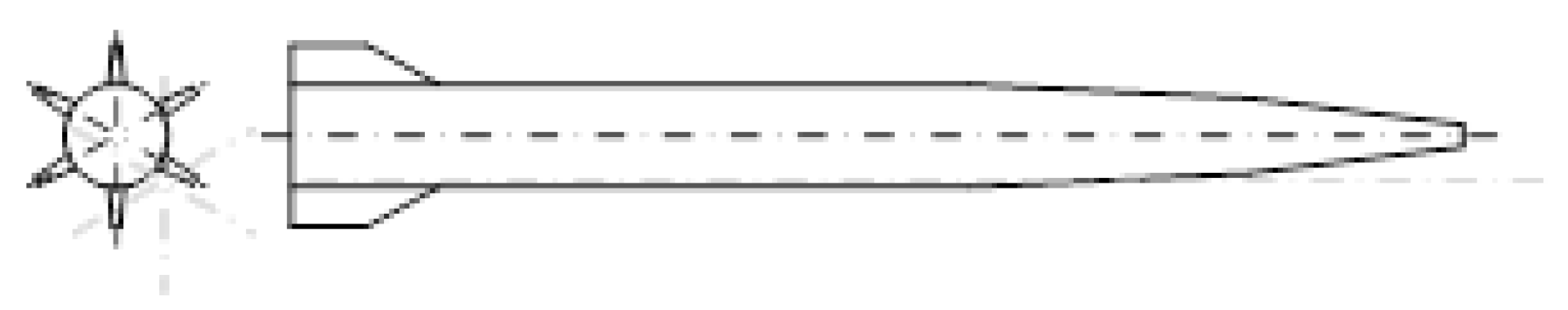
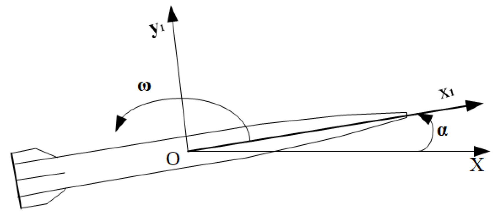
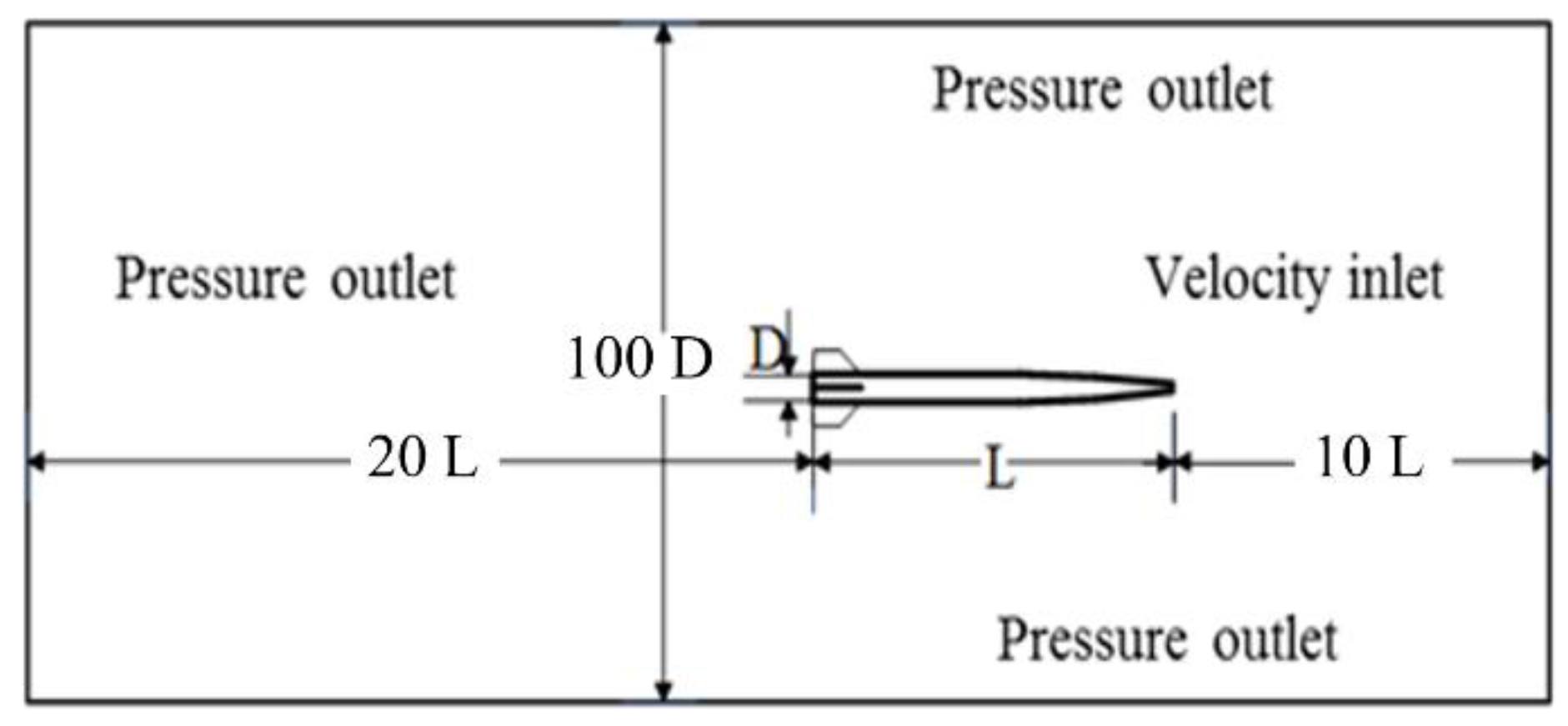
The high-speed supercavitation vehicle is a typical slender body, as shown in Figure 1. The front body is composed of two directly transitional cones, the middle is a cylinder, and the tail is equipped with six wings. The computing domain and boundary conditions are shown in Figure 2. Different cavitation number conditions are obtained by adjusting the incoming flow velocity. Based on the finite volume method, the fully implicit multigrid technique [19,20] is used to solve the momentum equation, continuity equation, and energy equation at the same time, and then scalar equations such as turbulence are solved. The transient term of the governing equation is discretized by a second-order implicit Euler scheme.

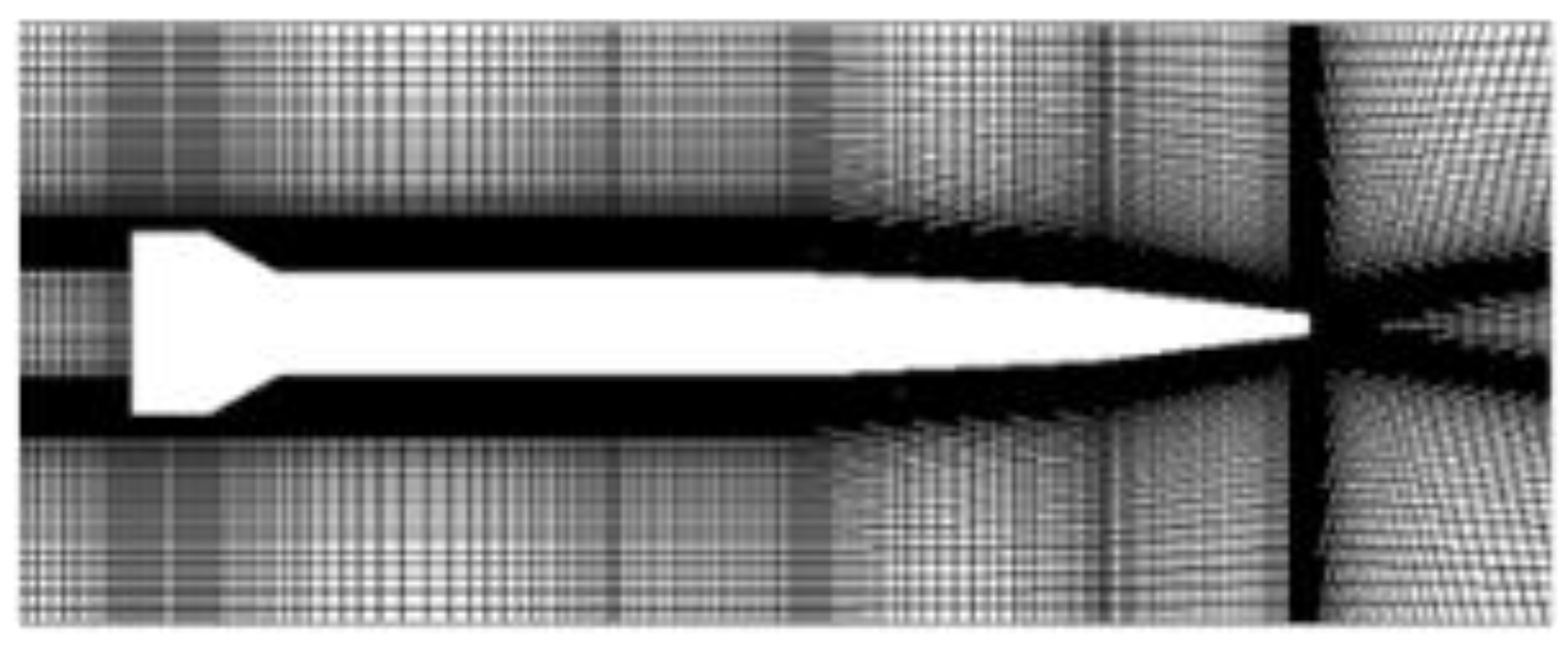
The computational mesh around the underwater vehicle is shown in Figure 3. The multiblock structured grids were used. The calculation domain is divided into two parts. The grid of the inner region is dense, and the outflow region is sparse, thus reducing the total number of grids and improving the calculation efficiency. These two regions are connected through the interface. The grid refinement algorithms are conducted in the boundary layer near the wall and the water–vapor interface. Moreover, adaptive mesh refinement according to the pressure and velocity gradient is utilized to accurately capture the evolution of the cavitation shape during the calculation.

3. Cavitation Flow Control Equation

3.1. Homogeneous Equilibrium Flow Model

Cavitation multiphase flow is involved in high-speed supercavitation. According to the published literature, the homogeneous equilibrium flow model is widely used in numerical simulations and performs well in predicting natural cavitation. Generally, there are two models, the mixture model and the VOF (Volume of Fluid) model, which are suitable for the natural cavitation and ventilated supercavity, respectively. For the mixture model, there is a unified velocity field and pressure field in the unit volume, and no relative velocity between the two phases is considered. The flow field density is determined by the volume fraction and density of the two phases. In this paper, natural cavitation is studied, so the mixture homogeneous equilibrium flow model is adopted. The main equations involved include the continuity equation, momentum equation, and energy equation.

(1)

The continuity equation:

$$\frac{\partial \rho }{\partial t}+\nabla •\left(\rho u\right)=0$$

(1)

$$\rho ={\displaystyle \sum }_{k=1}^n{\alpha }_k{\rho }_k$$

(2)

$$u=\frac{1}{\rho }{\displaystyle \sum }_{k=1}^n{\alpha }_k{\rho }_k{u}_k$$

(3)

where $\rho$ is the fluid mixing density; u is the mixing speed; and $n$ is the number of phases. Since noncondensable gas is considered, $n=3$, ${\alpha }_k$, ${\rho }_k$, and $u_k$ are the volume fraction, density, and velocity of the k-th phase.

(2)

The momentum equations:

$$\frac{\partial \left(\rho u\right)}{\partial t}+\nabla •\left(\rho uu\right)=-\nabla p+\nabla •{\tau }_{ij}+S$$

(4)

$${\tau }_{ij}=\mu \left[\left(\frac{\partial u_i}{\partial x_j}+\frac{\partial u_j}{\partial x_i}\right)-\frac{2}{3}{\delta }_{ij}\frac{\partial u_k}{\partial x_k}\right]\begin{array}{cc},& {\delta }_{ij}=\{\begin{array}{c}1\begin{array}{cc}& \left(i\ne j\right)\end{array}\\ 0\begin{array}{cc}& \left(i=j\right)\end{array}\end{array}\end{array}$$

(5)

$$\mu ={\displaystyle \sum }_{k=1}^n{\alpha }_k{\mu }_k$$

(6)

where $p$ is the pressure, and S is the source term. The term ${\tau }_{ij}$ represents the shear stress, which is written as (5). $\mu$ is the hybrid viscosity, and its expression is (6). ${\mu }_k$ is the dynamic viscosity of the k-th phase.

(3)

The volume fraction equation of water vapor phase:

$$\frac{\partial {\rho }_v{\alpha }_v}{\partial t}+\nabla •\left({\rho }_v{\alpha }_{v}u\right)={\dot{m}}^{+}+{\dot{m}}^{-}$$

(7)

where ${\rho }_v$ is the water vapor density, and ${\alpha }_v$ is the water vapor volume fraction. The term ${\dot{m}}^{+},{\dot{m}}^{-}$ represents the condensation rate and vaporization rate of water vapor, which are described in the cavitation model.

(4)

The energy equation:

$$\frac{\partial }{\partial t}{\displaystyle \sum }_{k=1}^n\left({\alpha }_k{\rho }_k{E}_k\right)+\nabla {\displaystyle \sum }_{k=1}^n\left({\alpha }_k{v}_k\left({\rho }_k{E}_k+p\right)\right)=\nabla \left[k_{eff}\nabla T\right]+S_E$$

(8)

$$E_k=h_k-\frac{p}{\rho }+\frac{v_k^2}{2}$$

(9)

$$k_{eff}={\displaystyle \sum }_{k=1}^n{\alpha }_k\left(k_k+k_l\right)$$

(10)

where the term $E_k$ represents the internal energy of the k-th phase; for a compressible flow, $E_k=h_k$; and $h_k$ is the apparent enthalpy of the k-th phase. $k_{eff}$ is the effective thermal conductivity, $k_l$ is the turbulent thermal conductivity, and $T$ is the local temperature.

3.2. Viscous Model

The flow around the high-speed supercavitation vehicle has strong turbulence characteristics. Therefore, the viscous model plays an important role in the simulation of turbulence. In this paper, the realizable k-ε model based on the RANS (Reynolds-Averaged Navier-Stokes) method is adopted. Moin [21] pointed out that the standard k-ε model may have negative positive stress when the time-average strain rate is large. Shin [22] combined $C_{\mu }$ and the strain rate in the turbulence formula to mathematically constrain the normal stress to ensure that the flow conforms to the physical laws and proposed a realizable k-ε model that is more in line with the actual situation. The modeled transport equations for k and $\epsilon$ in the realizable k-ε model are

$$\rho \frac{Dk}{Dt}+\frac{\partial \left(\rho k{u}_j\right)}{\partial x_j}=\frac{\partial }{\partial x_j}\left[\left(\mu +\frac{{\mu }_t}{{\sigma }_k}\right)\frac{\partial k}{\partial x_j}\right]+G_k+G_b-\rho \epsilon -Y_M+S_k$$

(11)

$$\rho \frac{D\epsilon }{Dt}+\frac{\partial \left(\rho \epsilon u_j\right)}{\partial x_j}=\frac{\partial }{\partial x_j}\left[\left(\mu +\frac{{\mu }_t}{{\sigma }_t}\right)\frac{\partial \epsilon }{\partial x_j}\right]+\rho C_{1}S\epsilon -\frac{\rho C_2{\epsilon }^2}{k+\sqrt{v\epsilon }}+C_{1\epsilon }\frac{\epsilon }{k}{C}_{3\epsilon }{G}_b+S_{\epsilon }$$

(12)

$$C_1=max\left[0.43,\frac{\eta }{\eta +1}\right],\begin{array}{c}\end{array}\eta =S\frac{k}{\epsilon },\begin{array}{c}\end{array}{\mu }_t=\rho C_{\mu }\frac{k^2}{\epsilon },\begin{array}{c}\end{array}$$

(13)

In these equations, $G_k$ represents the generation of turbulence kinetic energy due to the mean velocity gradients. $G_b$ is the generation of turbulence kinetic energy due to buoyancy. $Y_m$ represents the contribution of the fluctuating dilatation in compressible turbulence to the overall dissipation rate, and the term incompressible flow is 0. $C_2$ and $C_{1\epsilon }$ are constants. ${\sigma }_k$ and ${\sigma }_{\epsilon }$ are the turbulent Prandtl numbers for k and $\epsilon$, respectively. $S_k$ and $S_{\epsilon }$ are user-defined source terms. ${\mu }_t$ is the turbulent viscosity coefficient. In the realizable k-ε model, $C_{\mu }$ is a function of the strain rate and curl, and its value is 0.09 on the viscous bottom layer.

3.3. Cavitation Model

Cavitation models are widely used in CFD calculations. This type of model uses mass source terms to simulate the mass conversion between water and vapor, as well as the unsteady characteristics of flow. The Schnerr and Sauer model proposed in 2001 [23] is used in this article. This model relates the volume fraction of the vapor phase to the number of cavitations per unit volume of fluid. The expressions are

$$\{\begin{array}{c}{\dot{m}}^{+}=\frac{{\rho }_l{\rho }_v}{{\rho }_w}{\alpha }_{nuc}\left(1-{\alpha }_{nuc}\right)\frac{3}{R_B}\sqrt{\frac{2}{3}\frac{p_v-p}{{\rho }_l}}\begin{array}{cc}& p<p_v\end{array}\\ {\dot{m}}^{+}=\frac{{\rho }_l{\rho }_v}{\rho }{\alpha }_{nuc}\left(1-{\alpha }_{nuc}\right)\frac{3}{R_B}\sqrt{\frac{2}{3}\frac{p-p_v}{{\rho }_l}}\begin{array}{cc}& p>p_v\end{array}\end{array}$$

(14)

$$\{\begin{array}{l}{R}_B={\left(\frac{{\alpha }_{nuc}}{1-{\alpha }_{nuc}}\frac{3}{4\pi }\frac{1}{n}\right)}^{\frac{1}{3}}\\ {\alpha }_{nuc}=\frac{\frac{4}{3}\pi R_B^3{N}_B}{1+\frac{4}{3}\pi R_B^3{N}_B}\end{array}$$

(15)

where ${\dot{m}}^{+}$ is the evaporation rate. ${\dot{m}}^{-}$ is the condensation rate. ${\rho }_l$ and ${\rho }_v$ are the water and vapor densities, respectively. ${\rho }_w$ is the water density. ${\alpha }_{nuc}$ is the gas core volume fraction. $R_B$ is the gas core cavity diameter. n is the number of cavities per unit volume.

4. Verification of the Calculation Model

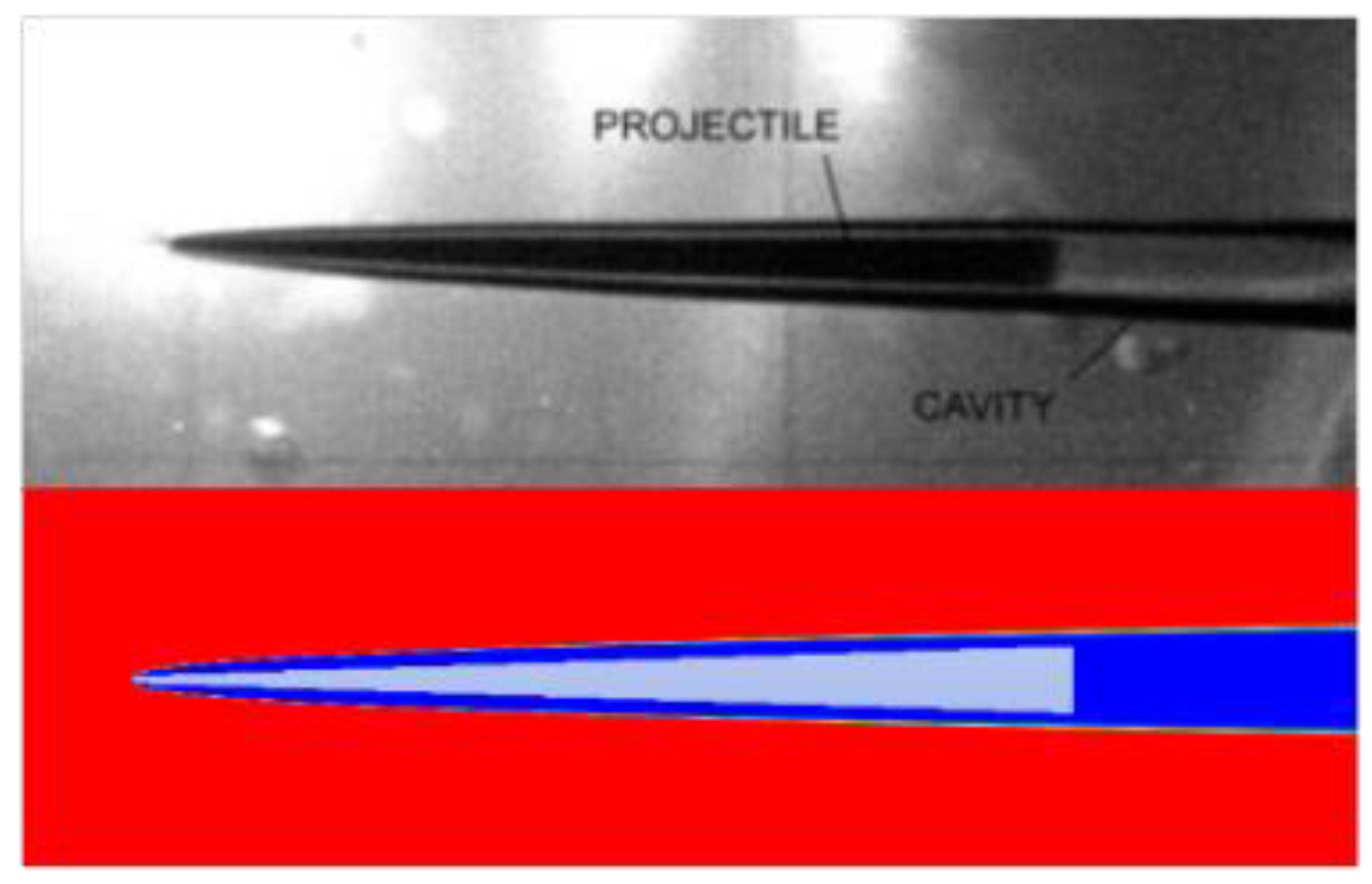
The numerical simulation method established above is evaluated for the supercavitation flow around a flat-headed conical vehicle (as shown in Figure 4). The experiment was conducted by Hrubes [24]. The test uses a 30 mm caliber underwater gun to launch at a depth of 4 m. The animation of the water entry process is taken by a high-speed camera. The laser is used to measure the velocity of a vehicle. In this paper, the simulation is carried out for the condition with a water depth of 4 m at room temperature and an incoming flow velocity of 970 m/s corresponding to a cavitation number of $\mathsf{\sigma }=2{\times 10}^{-4}$, which is defined as follows:

$$\mathsf{\sigma }=\frac{P_{\infty }-P_v}{\frac{1}{2}\rho V^2}$$

(16)

where $P_{\infty }$ and $P_v$ represent the environment pressure and the saturate pressure, respectively. $\rho$ is the density of the water, and V is the velocity of the main flow.

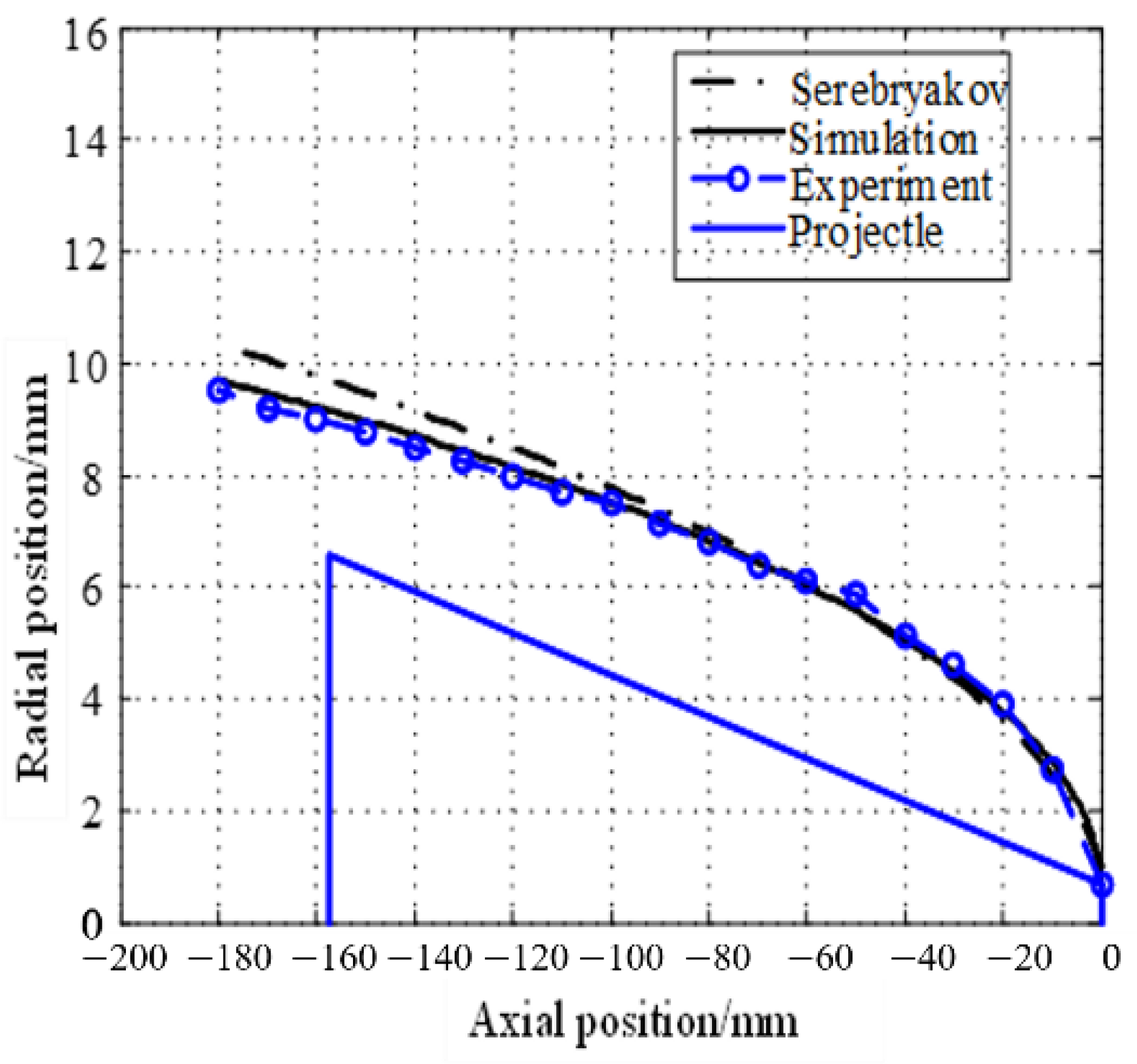
Figure 5 shows the comparison of the density distribution between the experimental and numerical results. The vehicle has been enveloped by the cavitation, showing an obvious state of supercavitation. The simulation result is in good agreement with the test result. Figure 6 shows the cavitation radius at different positions from the head of the cavitator calculated by the test, simulation, and semiempirical formula. The simulation of the supercavitation shape in this paper has good accuracy and high reliability. Therefore, the above numerical methods are further used in the later simulation of supercavitation flow.

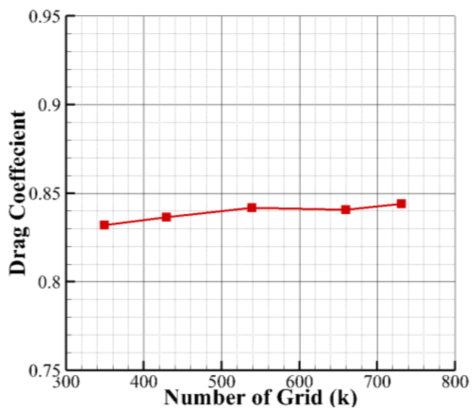
In addition, the drag coefficient obtained by using five different grids is shown in Figure 7. The numbers of grids are $3.5\times {10}^5$,$4.3\times {10}^5$,$5.4\times {10}^5,6.6\times {10}^5$ and $7.3\times {10}^5,$ respectively. The drag coefficient $C_d$ is defined as follows:

$$C_d=\frac{F_d}{\frac{1}{2}\rho V^{2}S}$$

(17)

where $F_d$ is the drag force, $\mathsf{\rho }$ is the density of the water, and V is the velocity of main flow. S is the area of the cavitator.

It can be observed that with the number of grids increasing, the drag coefficient rises slightly. When the number is larger than 540,000, the variety of the drag coefficient is within 0.5%. Therefore, the number of grids in this paper is set to 540,000, and the numerical simulation is validated.

5. Cavitation Evolution Characteristics of High-Speed Vehicles

Due to the high speed of the vehicle, such as with the ejection tube used for testing in Ukraine and the United States, the velocity is more than 1000 m/s, and the trajectory is relatively stable for horizontal straight navigation. However, for the condition with an attack angle, the projectile trajectory is extremely easy to be made unstable. Even a small attack angle below 1° would significantly affect the projectile motion and cavitation shape. Therefore, the flow field and cavitation shape of a projectile at high speed at different attack angles are studied and analyzed in detail in this paper. The incoming flow velocity considered ranges from 300 m/s to 1500 m/s, and the corresponding Reynolds number $\mathrm{Re}=\frac{VD}{\upsilon }$ ranges from about 450,000 to 2,250,000. The attack angle ranges from 0° to 3°. Due to the max diameter being small, the gravity effect is not considered in the numerical simulation. Therefore, the Froude number is not involved in this paper.

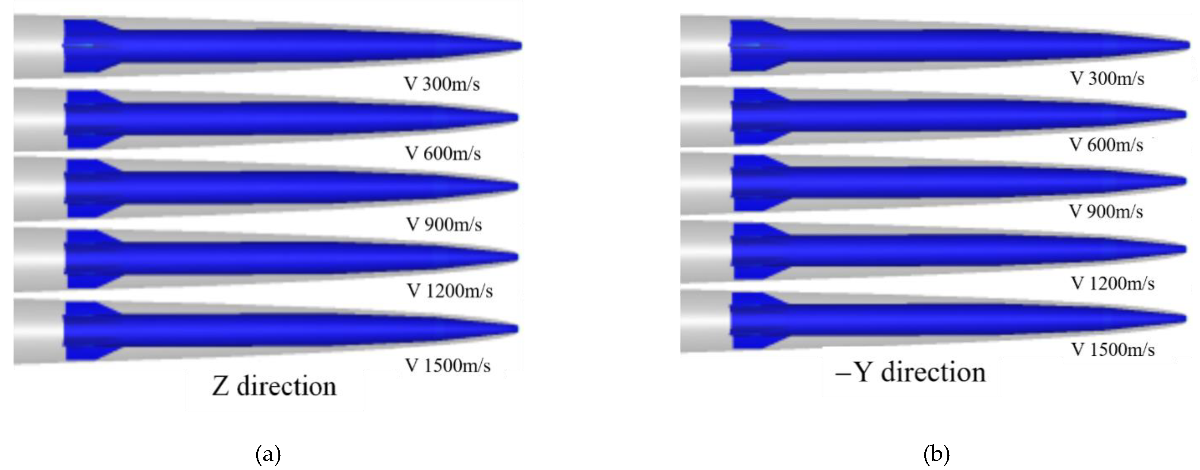
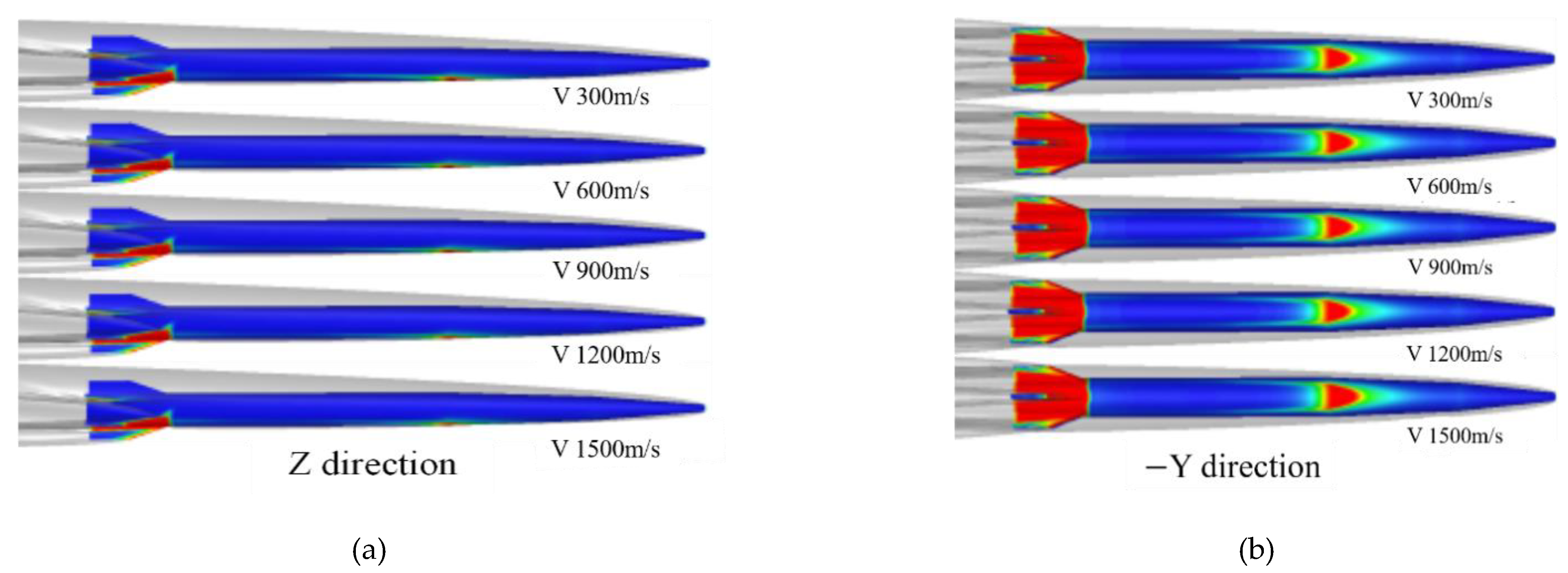
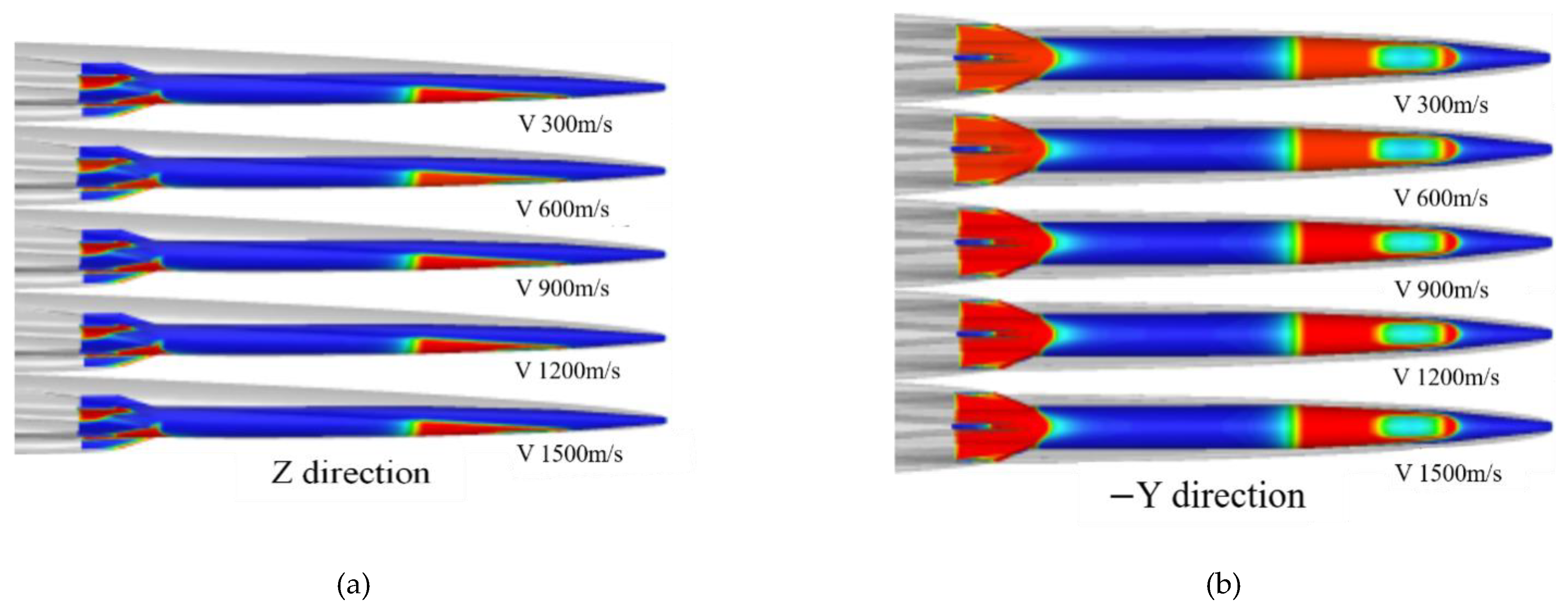
Figure 8, Figure 9, Figure 10 and Figure 11 show the density distribution on the projectile surface at different speeds and attack angles, as well as the comparison of the isosurface with the contour density surface of 500 kg/m³ (which is defined as the cavitation interface in this paper). The redder the color is, the greater the density is. In the local cavitation state, the cavitation number has a great influence on the cavitation shape. When supercavitation occurs (as shown by the equal density surface of 500 kg/m³), the shape of the cavitation around the projectile under different cavitation numbers is basically the same in the cases with the same attack angle.

When the speed is the same (300m/s), the attack angle has a significant effect on the shape of the cavity and its positional relationship with the projectile. With an increasing attack angle, the offset of the back surface of the cavitation increases significantly. When the attack angle is 0°, the projectile is cavitation-wrapped. As the attack angle increases to 1°, the wing is slightly wetted, indicating that the cavitation part is punctured, and a secondary cavitation appears near the wetted part of the wing. When the attack angle increases to 2° (as shown in Figure 10), the wing on the water-facing surface has been fully wetted, and the wetted area has transitioned to the body. The bottom cavities are fully pierced by the wing, but at the tip of the wing, they are still in a state of cavitation. In addition, the conical transition zone of the second part of the projectile also appears partially wet. When the attack angle is 3°, the conical transition zone of the first part of the projectile is wetted on a large scale, secondary cavitation appears, and the shape of the cavitation is more complicated. Therefore, as the attack angle increases, the cavitation on the water-facing surface is more severely compressed by the incoming flow, and the offset of the cavitation to the back surface becomes increasingly serious.

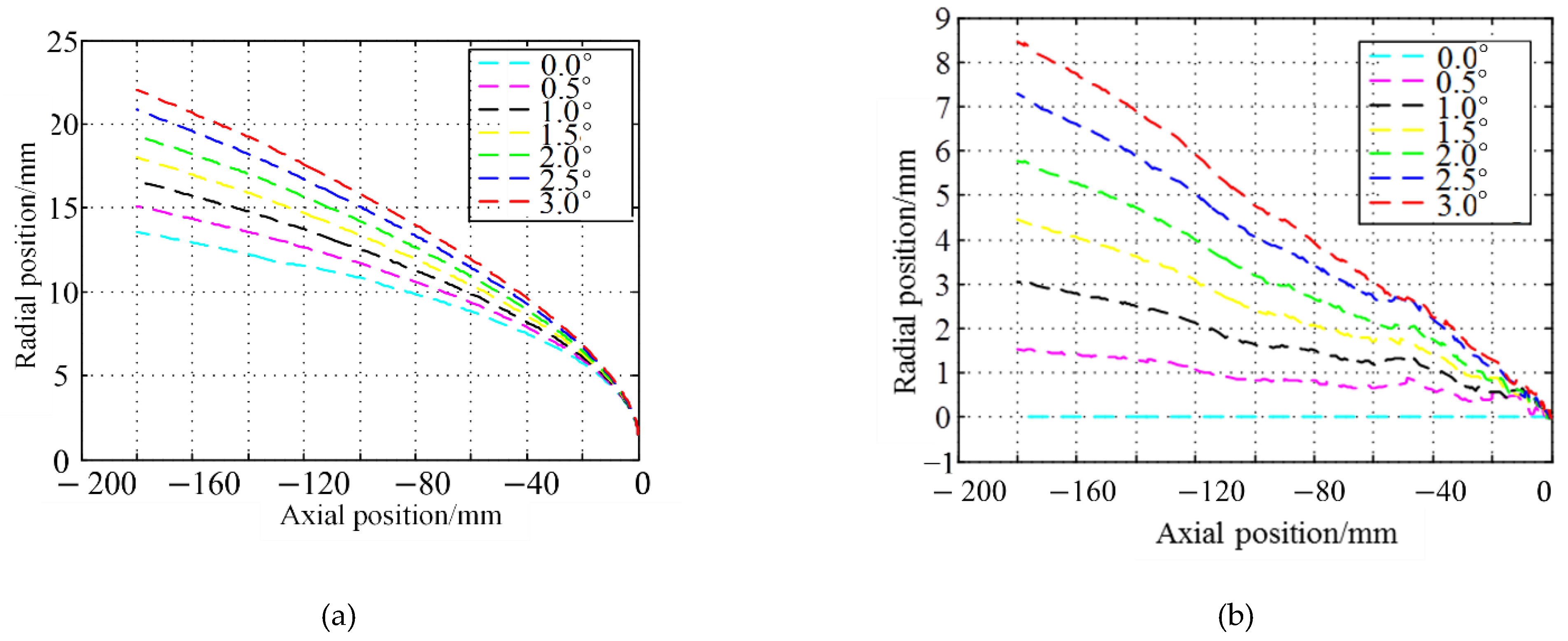
To quantitatively measure the magnitude of the offset, Figure 12a shows the comparison of the cavitation interface on the back water surface at different attack angles. From 0° to 3.0°, the upper boundary of the cavitation in the longitudinal plane continuously removes wards of nearly 9 mm. From the given radial offset distribution of the cavitation axis relative to the axis when the attack angle is 0° at each attack angle, it can be seen that at the same position, the larger the attack angle is, the greater the offset is. However, from the amount of change, the tendency of the increase slows down as the attack angle increases. At the same attack angle, the distance from the cavitator is also positively correlated with the offset, and the farther it is from the cavitator, the more violently the offset increases.

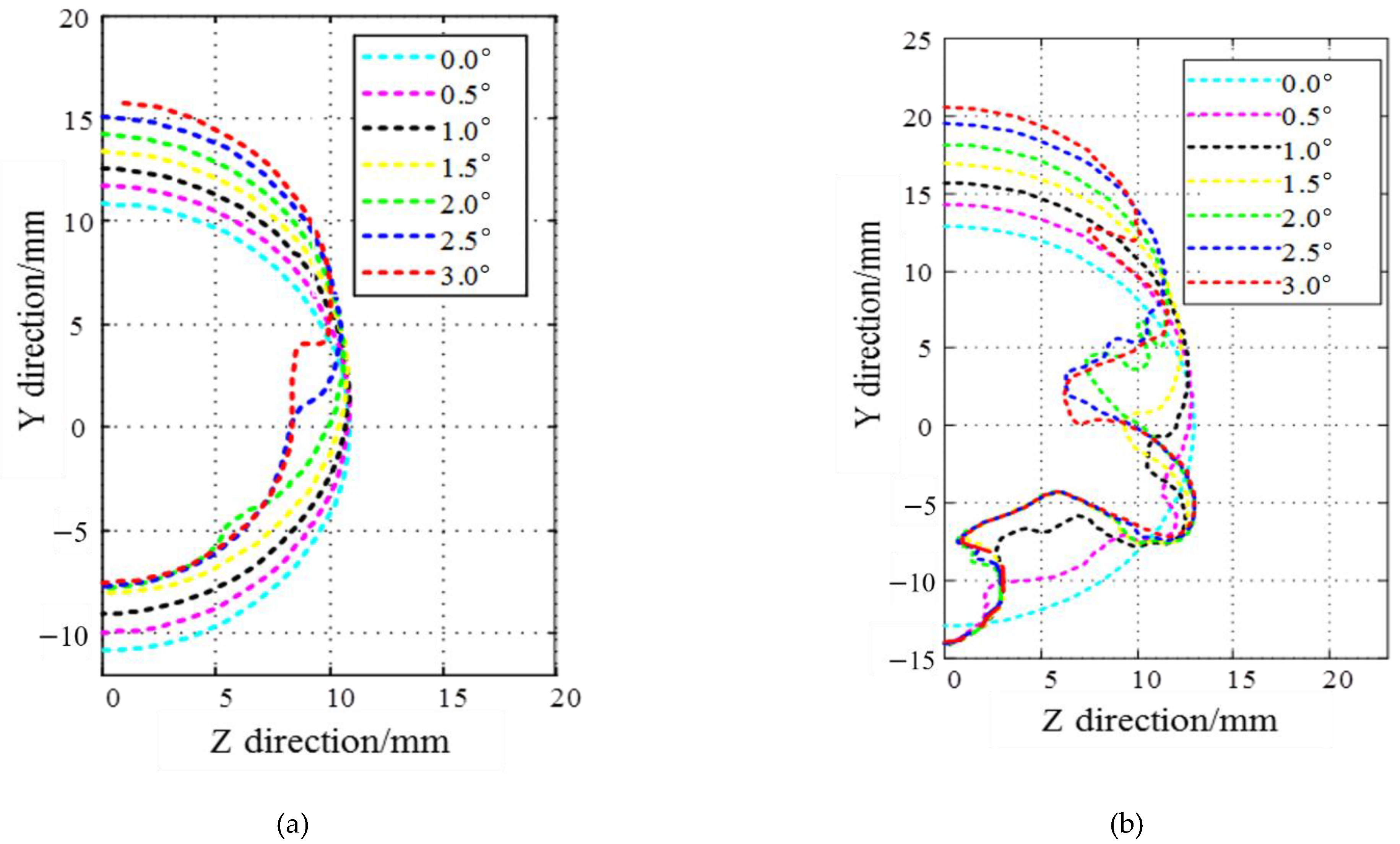
Figure 13 gives the comparison of the cavitation morphology of different axial cross-sections. The cross-section of the cavitation is a regular circular shape 100 mm behind the cavitation when the attack angle is 0°. With an increasing attack angle, the cross-sectional shape gradually changes to an ellipse. When the angle of attack increases to 2.0° and 2.5°, the shape is not smooth, and a pit appears. When the attack angle reaches 3°, the strong effect of the attack angle and secondary cavitation severely flattens and elongates the cross-section of the cavity, and an irregular contour appears, making the edge of the cavity more complicated.

Downstream of the projectile (160 mm behind the cavitator), a small attack angle (such as 0.5°) also causes the wing tip of the missile to wet and an accompanied secondary cavitation. Furthermore, at an attack angle of 3.0° the secondary cavitation is more pronounced. Therefore, the edge shape of the downstream cavitation is also obviously affected by the wing.

In summary, as the attack angle increases, the wetness of other parts starts from the bottom wing tip to the wing root, the tail of the projectile, the second part of the tapered transition zone, and the first part except for the foremost cavitator. In this process, every time a part of the wetted area is increased and the conditions for generating cavitation are reached, secondary cavitation will appear here, causing the flow field to become more complex, and the cross-sectional profile of the cavitation is more irregular. Flat and elongated cavities are added to the ellipsoid, and this situation becomes more serious as the attack angle increases.

6. Damping Characteristics Analysis of Ultrahigh-Speed Vehicles

Ignoring the inertial force, the hydrodynamic forces of the ultrahigh-speed vehicle when rotating or swinging in a fixed period include the position force and damping force. First, we conduct a numerical simulation study on the direct navigation conditions of ultrahigh-speed vehicles and obtain the position force characteristics in the longitudinal plane at different speeds and angles of attack. Comparing the direct sailing conditions with the oscillating conditions of the vehicle, the damping force characteristics of the ultrahigh-speed vehicle at a given angular velocity are obtained.

6.1. Position Force Characteristics of Ultrahigh-Speed Vehicles

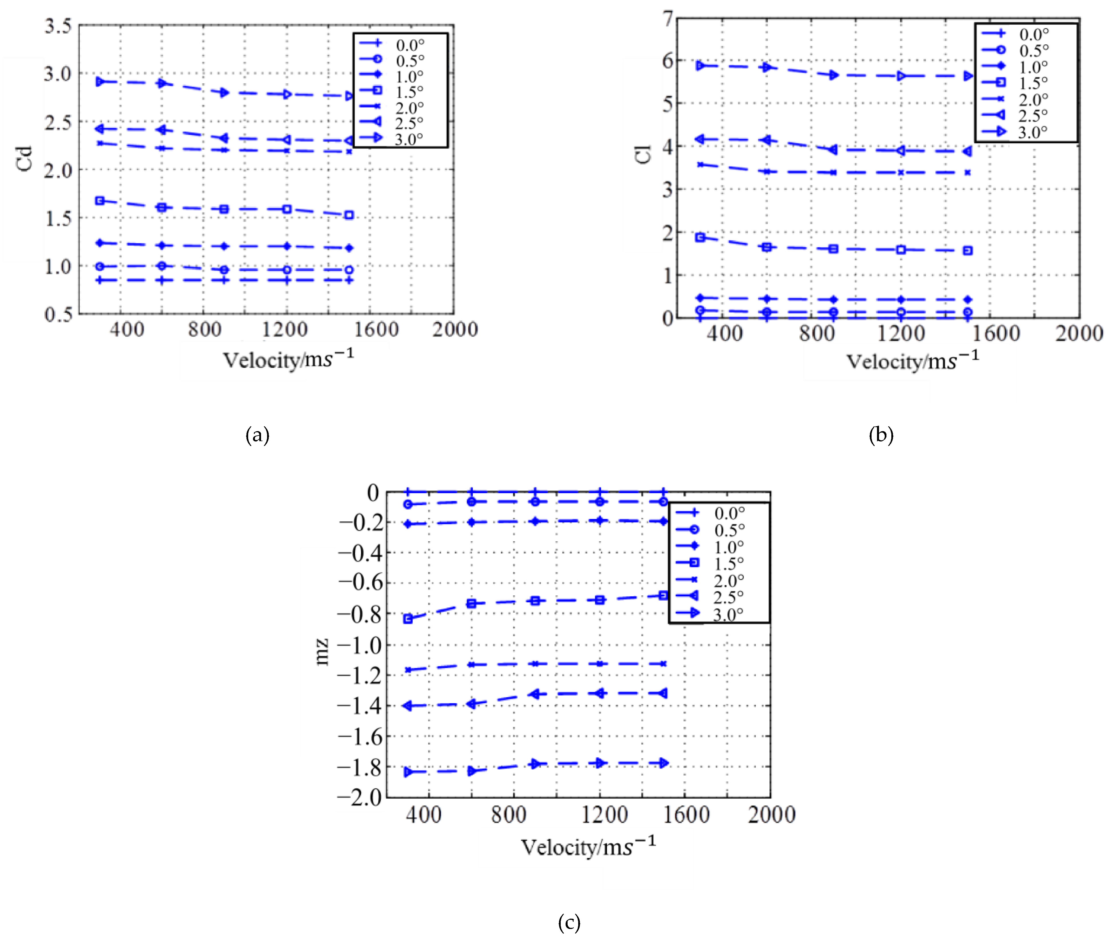
The variation in the hydrodynamic coefficient with the attack angle at different speeds under the direct navigation condition is shown in Figure 14. For a high speed with supercavitation, the vehicle is wrapped by cavitation, and the drag coefficient and lift coefficient are slightly affected by the speed when the attack angle is constant. With the change in attack angle, the hydrodynamic force of the projectile changes sharply. At the same speed, when the attack angle increases, the wetted state of the missile body and wing changes significantly (as shown in Figure 7, Figure 8, Figure 9 and Figure 10 above), so the fluid force (including resistance, lift, and pitch moment) changes accordingly. For example, as the attack angle changes from 0° to 3°, the drag coefficient increases sharply from 0.83 to 2.9, and the lift coefficient increases from 0 to 5.7.

In Figure 14c, since the wetted area at the tail of the wing is large, the lift generated on the after part of the projectile is larger than that generated by the cavitator and the conical transition zone at the front part, and an obvious negative value of the pitching moment coefficient is observed, resulting in a pitch down moment. Therefore, in the range of the attack angle, the given vehicle presents static stability characteristics, which are the excellent characteristics required by the supercavitation vehicle.

The changes in lift and pitching moment coefficients with attack angle and speed in Figure 14b,c are basically consistent with the changes in drag coefficient, which are all caused by the wetted area. The difference is that due to the larger wetting area of the tail of the wing projectile, the lift generated by the wing missile is larger than that generated by the cavitator and the tapered transition zone of the front end, which results in a significant negative value of the pitching moment coefficient, that is, a bowing moment. Within the range of the attack angle under study, the given ultrahigh-speed vehicle exhibits static and stable characteristics, which are the excellent characteristics required by the ultrahigh-speed vehicle.

6.2. Damping Characteristics of Ultrahigh-Speed Vehicle

Numerical simulations of the supercavitation vehicle oscillating periodically around the z-axis are carried out to study the damping characteristics. The swing of the supercavitation vehicle is shown in the Figure 15, The working conditions are as follows: sailing speed of 300 m/s, swing amplitude of 3°, and swing period of $T=4\mathrm{ms}$. The swing angle is calculated by Equation (18):

$$\alpha \left(t\right)=-\frac{3\pi }{180}\sin \left(500\pi t\right)$$

(18)

The user-defined function (UDF) provided by FLUENT is used for secondary development, and the projectile angular velocity is given to simulate the periodic swing. The time step is 0.02 ms, corresponding to 1/200 of the swing period. The damping force characteristics at the corresponding angular velocity and velocity are obtained by subtracting the hydrodynamic force at the corresponding attack angle and velocity from the direct navigation condition.

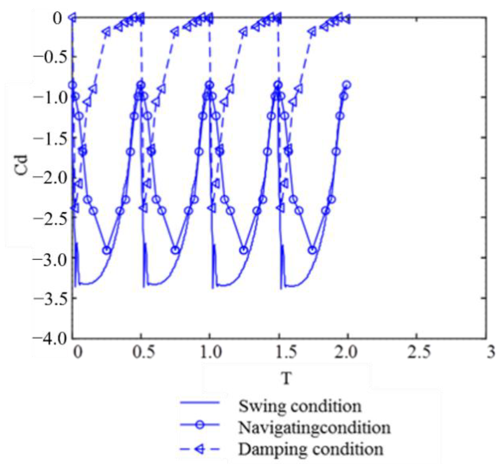
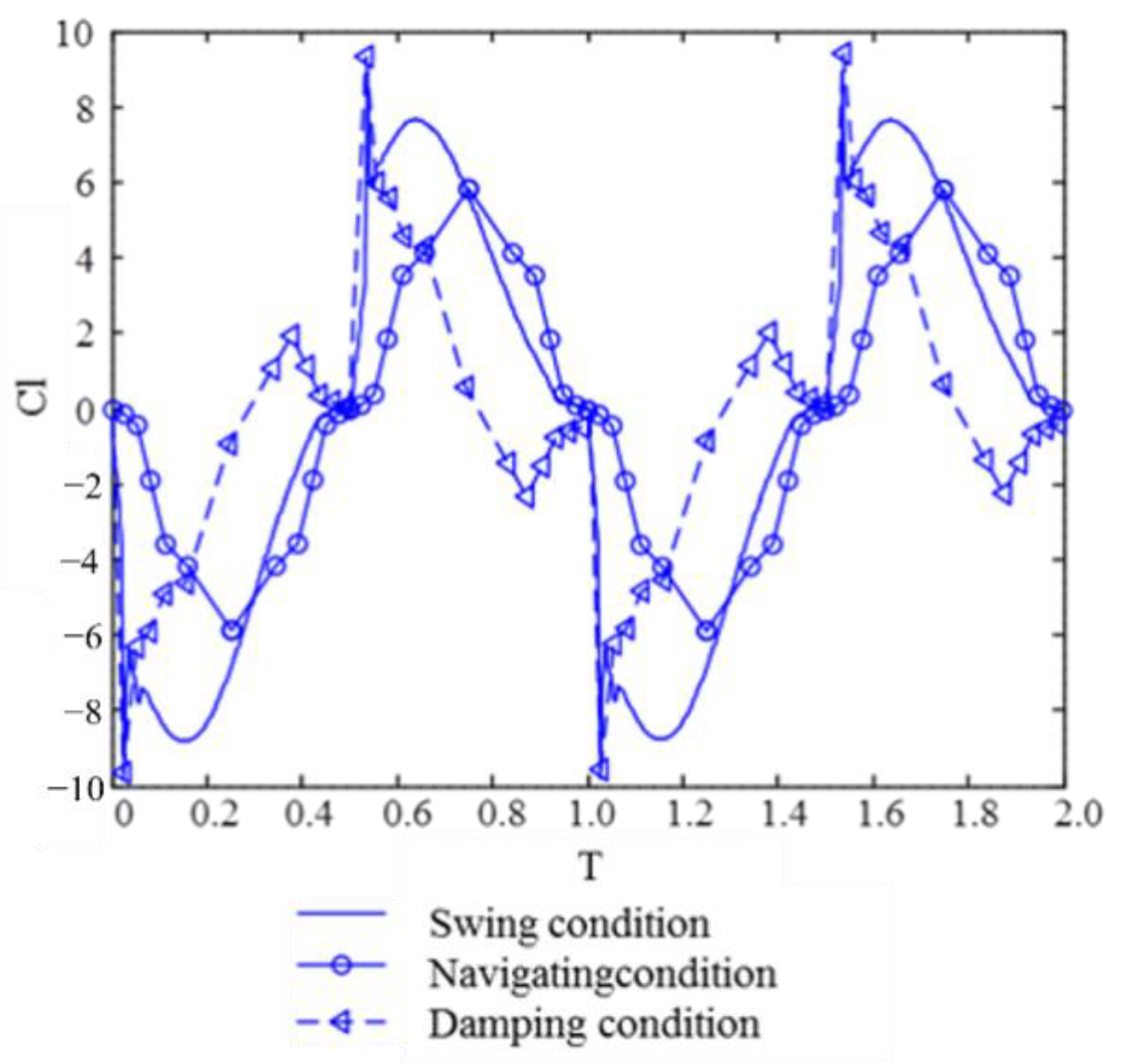
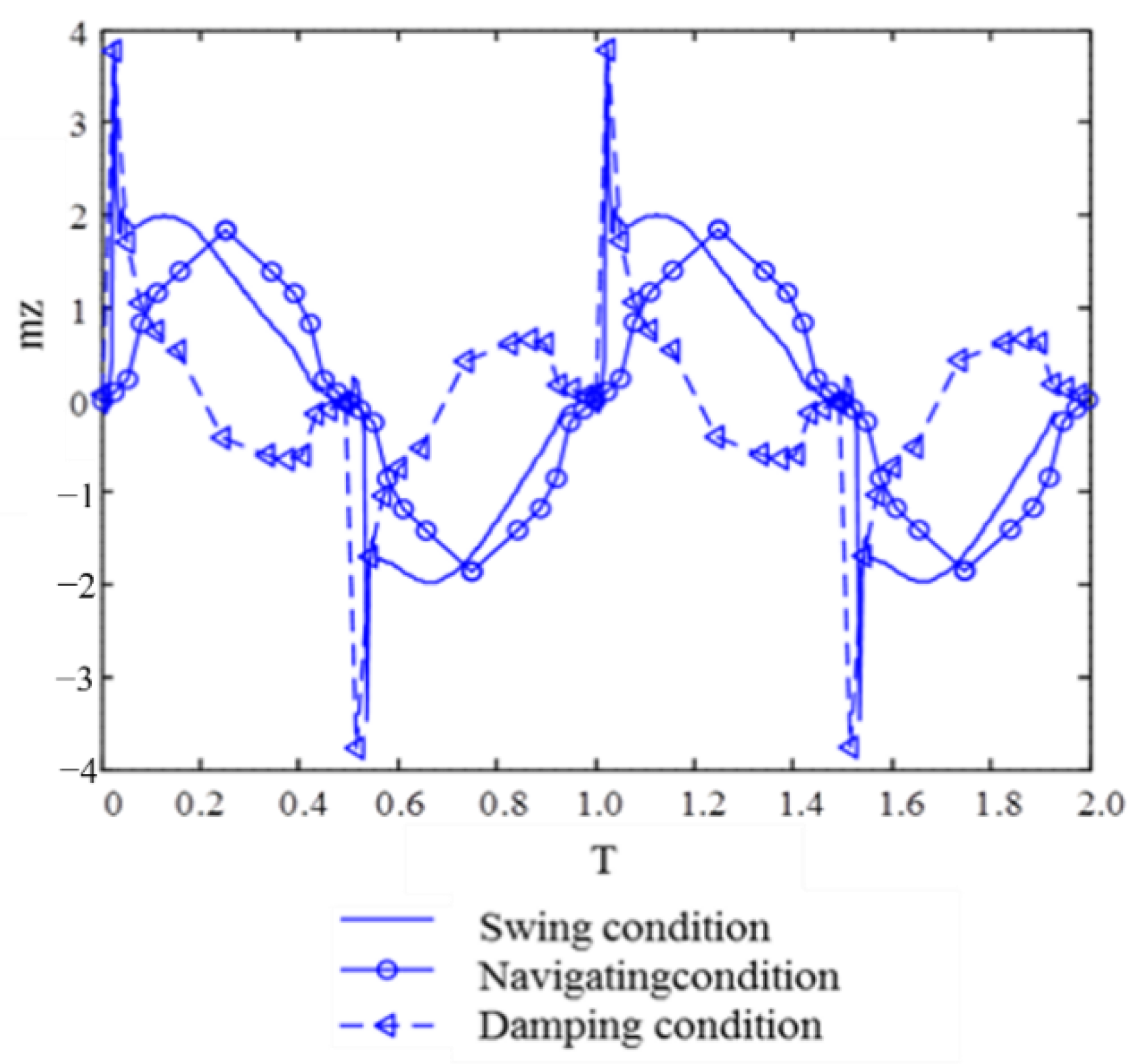
The coefficients of the high-speed supercavitation vehicle under periodic swing conditions are shown in Figure 16, Figure 17 and Figure 18. For comparison, the force and torque coefficients under constant direct navigation conditions are also given. Generally, when the high-speed vehicle swings periodically, the hydrodynamic force changes correspondingly. From Figure 16, as the attack angle of the vehicle first increases to the maximum value and then decreases, the resistance coefficient increases from small to large and then decreases accordingly. However, before the attack angle reaches the maximum, the maximum resistance coefficient is observed in advance. In Figure 17, the change in the lift characteristic is more complex than that of the drag coefficient. At the same angle, the lift coefficient is different in the process of raising the head and lowering the head. In addition, similar to the variation in the drag coefficient, the lift coefficient reaches the maximum value in advance before the attack angle reaches the maximum value.

From the change in pitching torque shown in Figure 18, at the beginning of the swing of the high-speed vehicle (or at a small attack angle), the shoulder is not wet, and the tail is slightly wet. During the continuous head-up motion of the vehicle, the damping force presents a positive effect on the motion, and then the torque coefficient quickly reaches the maximum value. When the head lowers, due to the hysteresis of the damping force, part of the position torque is offset. As a result, the change process of the torque is also relatively gentle.

Overall, the force and moment coefficients of the high-speed vehicle increase with increasing attack angle. In the swing process, due to the damping force, the variation of the force and moment coefficients with the attack angle is obviously different. When the vehicle gradually rises from zero, the damping force increases sharply to quickly reach the extreme value greater than that in direct navigation. When moving back from the maximum attack angle, the position force is partly offset by the damping force, thus delaying the variation of the force. Therefore, for the high-speed vehicle involved in the wet state, the damping term will have an important impact on the magnitude and the variation trend of the hydrodynamic force.

7. Conclusions

In this paper, the hydrodynamic characteristics of a high-speed vehicle under direct navigation at different speeds and angles of attack are simulated. Then, the damping force of the ultrahigh-speed vehicle during the periodic swing is analyzed. It can be concluded that:

(1)

When there is no wet surface on the surface of an ultrahigh-speed vehicle, its position force characteristics are less affected by the navigation speed. At the same velocity, with the increase of the attack angle, the wet area of the tail increases gradually, and then the fluid force is also enlarged. At the same attack angle as the wet surface, the drag coefficient decreases slightly with increasing velocity.

(2)

The hydrodynamic force changes roughly periodically according to the swing of the high-speed vehicle, whereas the maximum value is greater than that during the direct navigation state with the same attack angle.

(3)

The damping term has an obvious impact on the amplitude and change trend of the hydrodynamic force. When the high-speed vehicle gradually rises from a zero attack angle, the damping force plays a driving role. When it reaches the maximum attack angle and swings low, the damping force acts as an obstacle, and a hysteresis effect is observed for the force and torque coefficients.