Ionospheric Clutter Suppression with an Auxiliary Crossed-Loop Antenna in a High-Frequency Radar for Sea Surface Remote Sensing

Abstract

Ionospheric clutter is one of the main problems for high-frequency surface wave radars (HFSWRs), as it severely interferes with sea surface state monitoring and target detection. Although a number of methods exist for ionospheric clutter suppression, most are suitable for radars with a large-sized array and are inefficient for small-aperture radars. In this study, we added an auxiliary crossed-loop antenna to the original compact radar antenna, and used an adaptive filter to suppress the ionospheric clutter. The experimental results of the HFSWRs data indicated that the suppression factor of the ionospheric clutter was up to 20 dB. Therefore, the Bragg peaks that were originally submerged by the ionospheric clutters could be recovered, and the gaps in the current maps can, to a large extent, be filled. For an oceanographic radar, the purpose of suppressing ionospheric clutter is to extract an accurate current speed; the radial current fields that were generated by our method showed an acceptable agreement with those generated by GlobCurrent data. This result supports the notion that the ionospheric suppression technique does not compromise the estimation of radial currents. The proposed method is particularly efficient for a compact HFSWRs, and can also be easily used in other types of antennas.

1. Introduction

High-frequency surface wave radars (HFSWRs) have been widely used in the remote sensing of sea surface dynamic parameters and vessels, owing to the ability of high-frequency (HF) radio waves to propagate along the sea surface, and to resonate with the scattering of sea waves and ships [1,2]. A number of HFSWRs, e.g., the SeaSonde [3], the Wellen Radar (WERA) [4], and the Ocean State Measuring and Analyzing Radar (OSMAR) [5], have achieved success in oceanographic applications; however, in practice there may be some energy transmitted in directions other than the desired horizontal direction, which is reflected by the ionosphere, and then received by the radar. Consequently, ionospheric clutter may result from these undesired paths, forming a main problem for HFSWRs detection [6]. The ionospheric clutter should be well addressed in practice to ensure steady detection in performance.

A large number of effects and a few algorithms have been proposed for the HFSWRs [7] with regard to ionospheric clutter suppression [8,9], which have been reported to work well, and validated by real radar data. Working with multiple (dual) frequencies [10], whether in turn or simultaneously, can improve the detection of heavy clutters, but a high level of system complexity is required. The efforts based on a large array, e.g., adaptive beamforming [11], space–time adaptive processing [12], and polarization filtering [13], also lead to encouraging results, but their performances severely depend on the size of the array, and are thus inefficient for a compact radar. Some studies allow single-channel processing, such as time–frequency [14] and time–scale (wavelet) [15] filtering. They are effective in some specific situations, but may fail when the clutter is more widely distributed. To provide reference channels while keeping the compactness of the original array, a multi-layer, coaxial crossed-loop antenna was designed, which can be divided into two sets of sine-loops and cosine-loops [16]. By such a compact auxiliary antenna, the ionospheric clutter can largely be suppressed while preserving the first-order Bragg peaks; however, this method uses the different signals between loops of the same type on different layers, and thus requires an accurate calibration between the channels, which is often difficult to realize. Moreover, the involved least mean square (LMS) algorithm is relatively sensitive to the selection of learning rate. For an oceanographic radar, ionospheric clutter suppression is mainly aimed at the improvement of sea surface remote sensing [17]. The above literature only analyzes the ability to suppress ionospheric clutter, and does not verify whether the algorithm affects the subsequent remote sensing of sea surface dynamic parameters, such as the current.

In this study, we focused on the ocean surface current inversion, which is submerged in Es-layer ionospheric clutter. In order to improve the performance of ionospheric clutter suppression, we followed the clutter suppression method [16] with an auxiliary crossed-loop antenna for an OSMAR-S system, but simplified the structure of the adaptive filter and adopted the recursive least squares (RLS) filtering algorithm instead. The remainder of the paper is organized as follows: Section 2 describes the signal model and the adaptive filter; in Section 3, the experimental results are described and discussed; finally, conclusions are drawn in Section 4.

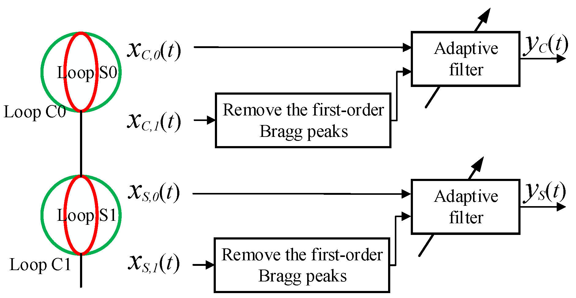
2. Signal Model and Adaptive Filter

Consider a double-layer crossed-loop antenna deployed in the same direction with a vertical spacing of d, where the upper layer is used as the main antenna and the lower layer as the auxiliary antenna, as shown in Figure 1.

According to their orthogonal normal directions, the double-layer crossed-loops can be divided into two pairs, namely, C-pair and S-pair. The directional patterns of the main crossed-loop can be denoted as:

$$a_{C,0}(\theta ,\phi )=\cos \phi$$

(1)

$$a_{S,0}(\theta ,\phi )=\sin \phi$$

(2)

where θ and φ are the angles of incidence and azimuth, respectively. The patterns of the auxiliary crossed-loop are:

$$a_{C,1}(\theta ,\phi )=\cos (\phi )e^{-jkd\cos \theta }$$

(3)

$$a_{S,1}(\theta ,\phi )=\sin (\phi )e^{-jkd\cos \theta }$$

(4)

where k is the wave number of the radar.

The received signals can thus be expressed as:

$$x_{C,m}(t)=s_C(t)+{\displaystyle \sum _{i=1}^N{z}_i(t)a_{C,m}(\theta ,\phi )}+n_{C,m}(t)$$

(5)

$$x_{S,m}(t)=s_S(t)+{\displaystyle \sum _{i=1}^N{z}_i(t)a_{S,m}(\theta ,\phi )}+n_{S,m}(t)$$

(6)

where m = 0, 1 (0 corresponds to the main crossed-loop and 1 to the auxiliary pair), $s_C(t)$ and $s_S(t)$ are the sea echo signals on the C-pair and S-pair, respectively, from the horizontal direction, $z_i(t)$ is the i’th component of the ionospheric clutter, assumed here to consist of N discrete sources, and $n_{C,m}(t)$ and $n_{S,m}(t)$ are the noises on the C-pair and S-pair, respectively.

In [16], the different signals between the two layers were obtained to cancel out the horizontal sea echoes, and thus an accurate calibration of the loop amplitudes was needed, which is difficult to realize. However, we found through the experiment that this step is unnecessary if the first-order Bragg peaks are removed first. Consequently, the filter structure can be greatly simplified, as shown in Figure 1. Here, the RLS algorithm is used in the adaptive filters, whose output errors are the final signals after the clutter suppression. Then, radial-current vectors are extracted from these signals by direction, finding for each Doppler component within the first-order Bragg peaks.

3. Experimental Results

3.1. System Parameters

The proposed method was tested by a real dataset which contained ionospheric clutters. The dataset was collected by an OSMAR-S system modified with an extra layer of auxiliary crossed-loops and two receiving channels, correspondingly. The OSMAR-S is a compact HFSWRs, whose main parameters of the experimental system are listed in

Table 1. Radar parameters.

Parameters	Values
Waveform	Frequency-modulated interrupted continuous wave (FMICW)
Working frequency	7.75 MHz
Bandwidth	30 kHz
Sweep period	0.27 s
Range resolution	5 km
Coherent integration time	4.6 min (1024 sweeps)
Main antenna	Crossed-loop/monopole
Auxiliary antenna	Crossed-loop
Layer spacing	2.94 m

. The experiment was carried out on a coastal experiment in Zhangpu, Fujian Province, China on 1 April 2013. An example of the range-Doppler (RD) spectrum is shown in Figure 2; heavy clutters can be observed, which had large extensions in both the range and Doppler dimensions, i.e., mainly from 75 to 245 km, and from −1 to 1 Hz, respectively. Part of the Bragg peaks (i.e., the vertical strips near ±0.27 Hz) were submerged by the ionospheric clutters, which may have caused a decrease in the detectable range. It is noticeable that far-away ionospheric clutters can be folded onto near-range bins due to the radar waveform, i.e., the frequency-modulated interrupted continuous wave (FMICW). The folding range for these data was 100 range bins, or equivalently 500 km.

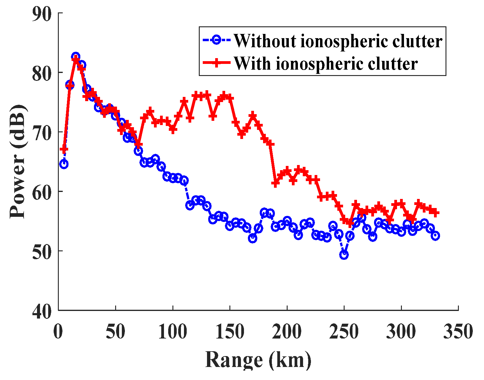
3.2. Detection of Ionospheric Clutter

The suppression process should be performed only when it is needed, since there may also be a loss in the signal of interest itself. Therefore, the detection of the ionospheric clutter was performed before the suppression began. For this purpose, the range spectrum in each dwell of coherent integration time (CIT) was calculated. When there were no ionospheric clutters, the range spectrum decreased monotonically, with an increasing range. However, when there were ionospheric clutters, the range spectrum showed abnormal rises at some specific ranges, e.g., 100–120 km for clutters from the sporadic E (Es) layer, and above 210 km for those from the F layer. Examples of the range spectra in both cases (without clutter at 00:24 and with clutter at 00:57 on 1 April 2013) are shown in Figure 3. By comparison with the threshold, which varied with the range, the ionospheric clutters were detected and the range bins, where they appeared, could thus be determined. It should be pointed out that the unnatural drop of the spectral power at the first two range bins was due to the blanking pulse of the radar for better isolation between transmitting and receiving, and that the final steady state, after about 200 km when there were no clutters, was corresponding to the noise floor.

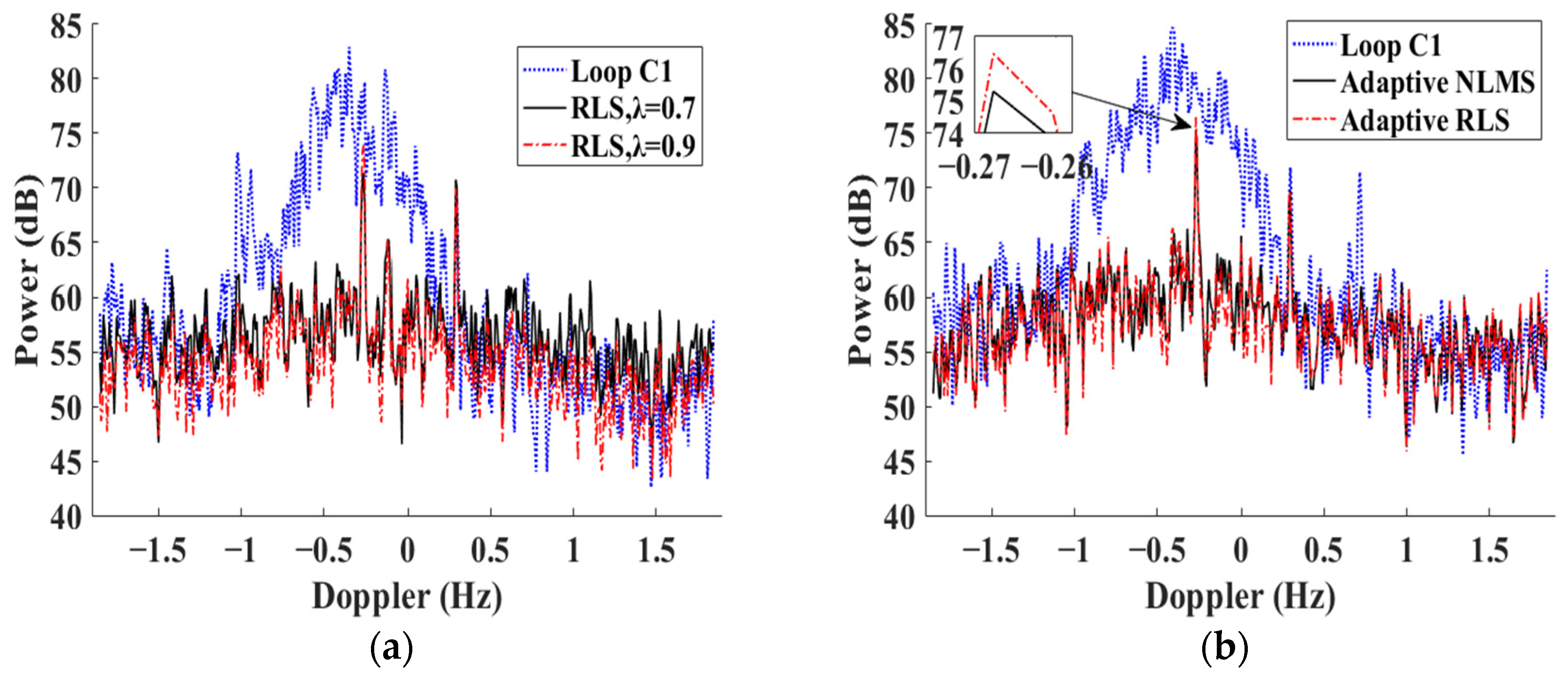
3.3. RLS Adaptive Filter

The RLS algorithm [18,19] has the advantage of a fast convergence speed, high estimation accuracy and good stability; therefore, it is widely used in the field of noise elimination. In this study, the RLS algorithm was used to update the weights of the adaptive filter. The performance of RLS has been well studied and proven to outperform LMS in both convergence and sensitivity to the updating rate.

Figure 4 shows the processing results of the Doppler spectrum at 95 km on Loop C1 at 0:57 on Apr 1, 2013, which is contaminated by ionospheric clutters. Different forgetting factors, e.g., $\lambda$ = 0.7 and $\lambda$ = 0.9, were tested to select the best forgetting factor for this scenario. As can be seen from Figure 4a, the proposed method performs well with both forgetting factors, and the improving factors of the signal-to-clutter ratio (SCR) have both been increased with a factor up to 20 dB. The Bragg peak near −0.27 Hz that was originally submerged by the ionospheric clutter was well recovered. The differences between the results of the different forgetting factors are small, but the improvement factor with $\lambda$ = 0.9 is greater. Thus the forgetting factor of the RLS filter hereafter was set to 0.9.

The RLS algorithm is also compared with the normalized LMS (NLMS) algorithm. The ionospheric clutter suppression results are shown in Figure 4b; here, the learning rate of NLMS is 0.1. We can see that the clutters have almost been suppressed completely by both algorithms, but the RLS algorithm has a smaller (about 1 dB) loss than the NLMS algorithm. Therefore, the RLS algorithm was a better choice for this study.

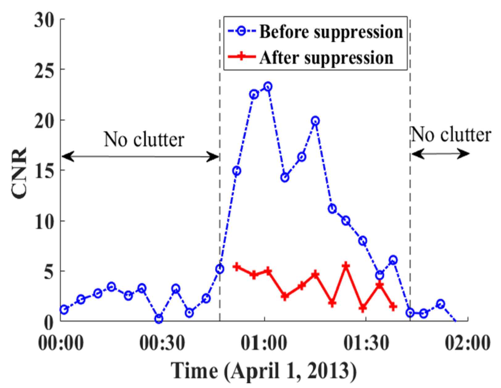
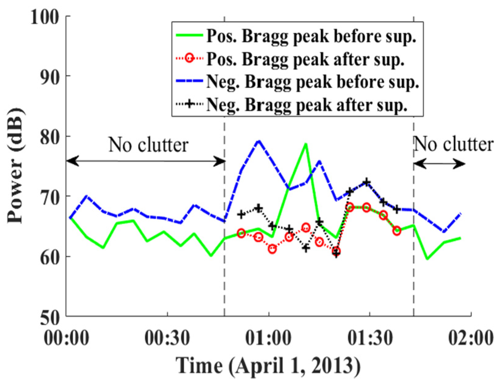
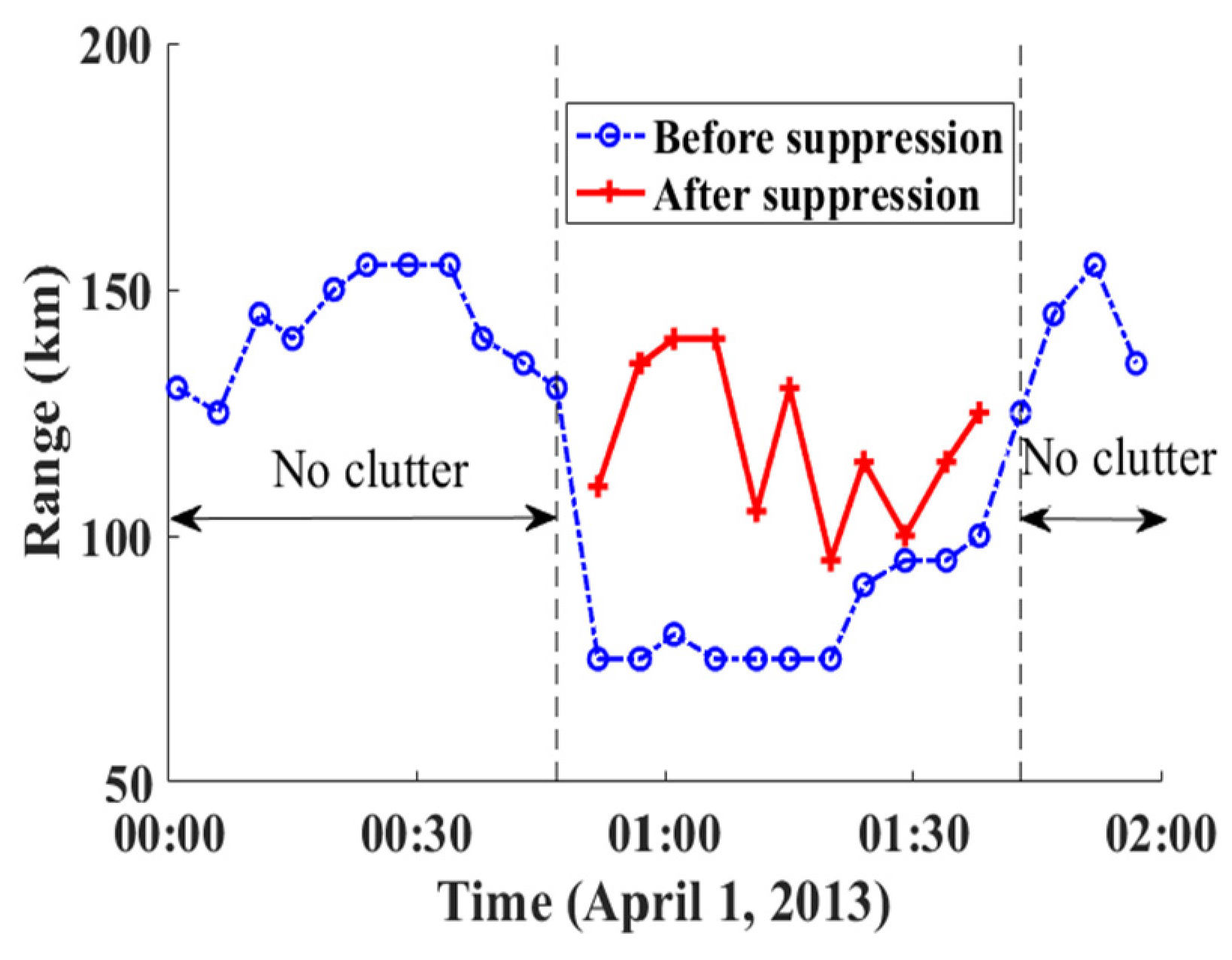
3.4. Suppression Performance

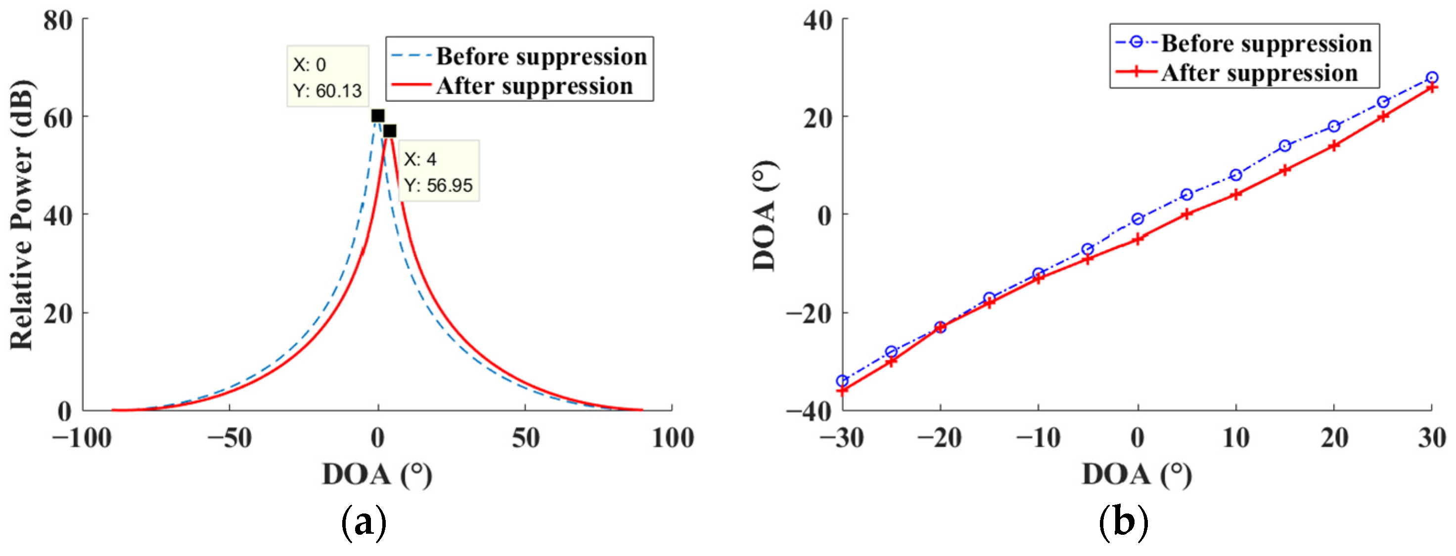
Since the ionospheric clutters may present various forms at different ranges and times, the power and SNR of the Bragg peaks, the correlation across ranges, and the maximum range valid for the current extraction were further evaluated to better understand the performance of the proposed method.

The RD spectrum that was shown in Figure 2 is given in Figure 5 after the clutter suppression, and the improvement in data quality is obvious. The vertical strips of the first-order Bragg peaks from 75 to 140 km, originally submerged by the clutters, were recovered to a large extent. The simultaneous improvements at both loops of the main antenna also ensured the feasibility of the subsequent current mapping from the recovered signals.

The dataset in this study covers a full course, from the emergence to the disappearance of the ionospheric clutters, and the overlapping between the ionospheric clutters and the Bragg peaks that exist throughout the appearance of the clutters. Figure 6 shows the decrease in the clutter-to-noise ratio (CNR) after the clutter suppression. The CNRs were originally from 5 to 24 dB, but decreased to below 5 dB, whether the clutter was strong or not. The final improvement factors were between 1 and 19 dB, which proved the effectiveness of the suppression.

Since the Bragg peaks played a vital role in the current mapping, their powers, and thus the signal-to-noise ratio (SNR), were important indices to evaluate the suppression performance. For the data in Figure 5, the spectral power series of the positive and negative Bragg peaks at 80 km after clutter suppression were respectively counted, as shown in Figure 7. It can be seen that both the positive and negative Bragg peak power series were recovered to a relatively steady state. This result indicated that the signals of interest could be recovered without an obvious loss after the processing.

In the sea–current mapping process of OSMAR-S, a minimum SNR of 10 dB is required at each range bin. Therefore, the ionospheric clutter suppression can improve the detection range of sea currents. The maximum detection ranges before and after the suppression are shown in Figure 8. As can be seen, the improvement of the detection range is between 5 and 65 km, and the detection ranges have been recovered to be near the average value, i.e., 140 km, when there are no ionospheric clutters.

3.5. DOA Estimation

In order to further study whether the ionospheric clutter suppression algorithm affects the subsequent direction of arrival (DOA) estimation, one target was added into the echo in the 14th range bin. The target was added to the Doppler frequency of 0.387 Hz in azimuth of −30° to 30°, respectively. The results of the DOA estimation are shown in Figure 9. It can be seen that the difference between the two results is less than 5°. Therefore, this algorithm does not affect the DOA estimation of compact HFSWRs.

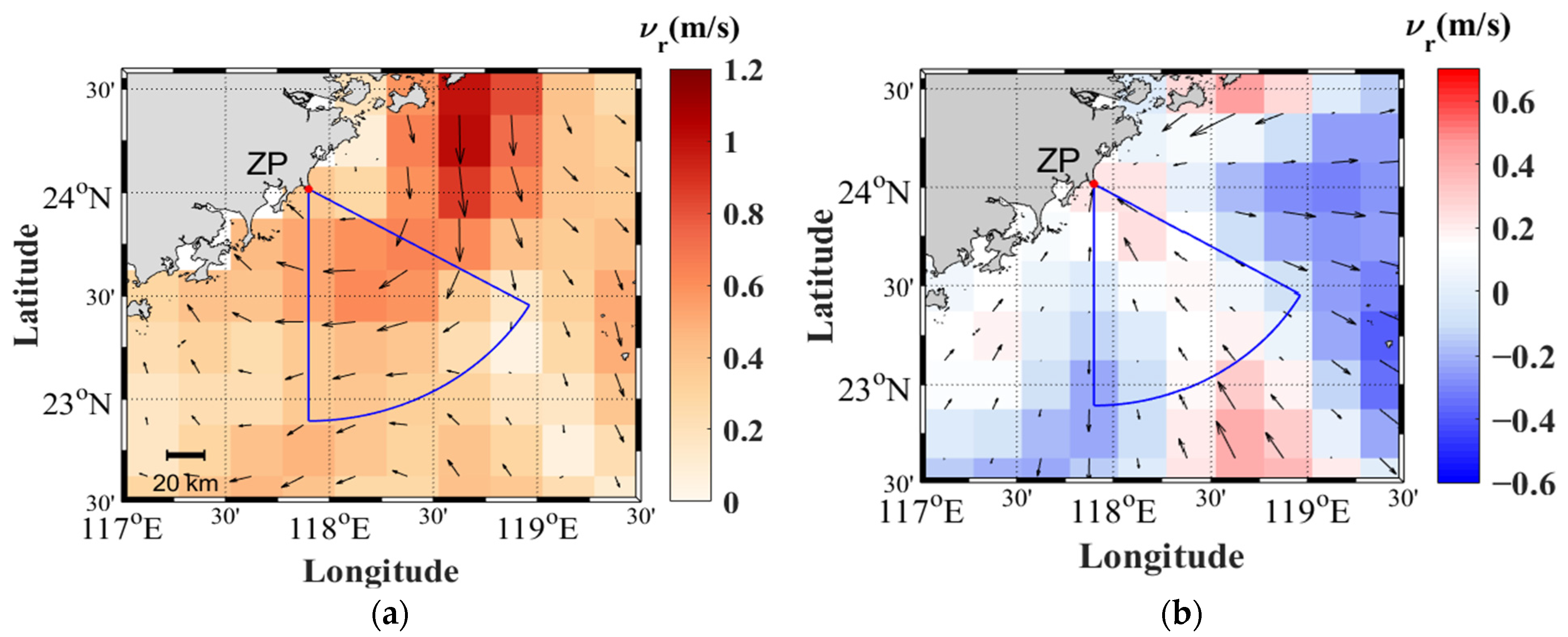
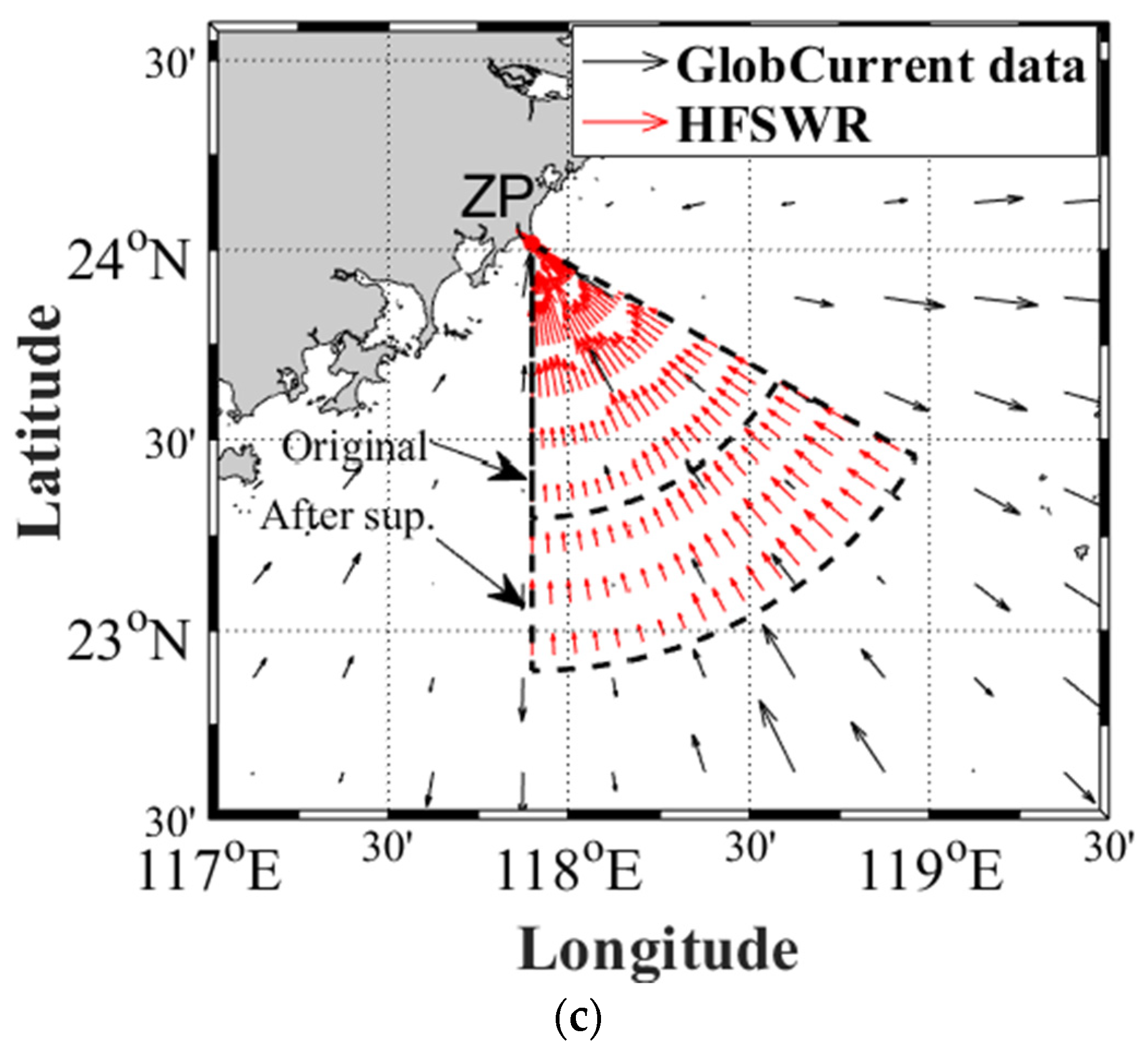
3.6. Recovered Current Map

No in situ buoy data were available for comparison in the experiment due to the limited experimental conditions. At present, GlobCurrent data can be applied for comparison to show the effect of the ionospheric clutter suppression. The GlobCurrent data can provide a temporal resolution of 3 h, and a spatial resolution of 0.25 degrees. It covers the 23-year period from 1993 to 2016 [20,21]. The dataset can provide the surface, the Ekman current, and the combined geostrophic and Ekman currents; generally speaking, the current in the Taiwan strait is generated by many factors, so the total surface current dataset is more suitable for algorithm validation. The HFSWRs measured data on 1 April 2013 from 00:01 to 01:57, so we chose the GlobCurrent data from 00:00 as the reference point. Figure 10a shows the GlobCurrent total current field at 00:00. Figure 10b shows the radial current at 00:00 provided by GlobCurrent.

For an oceanographic radar, the ionospheric clutter suppression is mainly aimed at the improvement of the current map. After the ionospheric clutter suppression is performed for each element of the main antenna, the sea-current-extraction algorithm [22] is applied to obtain the radial-current map. After the suppression, the maximum range of the radial-current map at 01:15 on 1 April 2013 was increased by 45 km, in agreement with the improvement in the detection range mentioned above. The HFSWRs radial current and GlobCurrent radial current at 00:00 are shown in Figure 10c. Moreover, to further show the reliability of the recovered sea currents, the time series of the radial currents at a range of 85 km in the direction of 0° is shown in Figure 11. The HFSWRs radial-current changes near the GlobCurrent radial current indicated that the radar measurement results after the ionospheric clutter suppression were in good agreement with the global radial current.

4. Conclusions

In this study, an improved method for ionospheric clutter suppression based on an auxiliary layer of crossed-loop antenna was proposed. The adaptive filter structure was simplified, and the RLS algorithm was adopted, which was fast converging and insensitive to the selection of the forgetting factor. The experimental results showed that the method was efficient in suppressing the strong ionospheric clutters with a large spread in both the range and Doppler dimensions, and the data quality was greatly improved after the suppression. The sea surface currents were further extracted from the recovered first-order Bragg peaks, which led to an increase of 45 km in the detection range. The auxiliary antenna structure could easily be extended to multiple layers, with the prospect of further improvement.

The proposed ionospheric clutter suppression algorithm was applied to the experimental compact HFSWRs data to compare the inverted ocean surface radial currents before and after the ionospheric clutter suppression. The results showed that the effective current detection range was significantly improved. Moreover, the comparison with the radial-current field generated by the GlobCurrent model showed an acceptable agreement, supporting the conclusion that the ionospheric suppression technique does not compromise the estimation of radial currents. Our future work will include more experiments for a better performance of sea current extraction under heavy ionospheric clutters.

References

1. Barrick, D.E. Remote sensing of sea state by radar. In Proceedings of the Ocean 72nd IEEE International Conference on Engineering in the Ocean Environment, Newport, RI, USA, 13–15 September 1972; pp. 186–192. [Google Scholar] [CrossRef]
2. Park, S.; Cho, C.J.; Ku, B.; Lee, S.; Ko, H. Compact HF Surface Wave Radar Data Generating Simulator for Ship Detection and Tracking. IEEE Geosci. Remote Sens. Lett. 2017, 14, 969–973. [Google Scholar] [CrossRef]
3. Lipa, B.; Nyden, B. Directional wave information from the SeaSonde. IEEE J. Ocean. Eng. 2005, 30, 221–231. [Google Scholar] [CrossRef] [Green Version]
4. Wyatt, L.R.; Mantovanelli, A.; Heron, M.L.; Roughan, M.; Steinberg, C.R. Assessment of Surface Currents Measured With High-Frequency Phased-Array Radars in Two Regions of Complex Circulation. IEEE J. Ocean. Eng. 2018, 43, 484–505. [Google Scholar] [CrossRef] [Green Version]
5. Lai, Y.; Zhou, H.; Zeng, Y.; Wen, B. Accuracy Assessment of Surface Current Velocities Observed by OSMAR-S High-Frequency Radar System. IEEE J. Ocean. Eng. 2018, 43, 1068–1074. [Google Scholar] [CrossRef]
6. Yang, X.; Wang, M.; Huang, W.; Yu, C. Experimental Observation and Analysis of Ionosphere Echoes in the Mid-Latitude Region of China Using High-Frequency Surface Wave Radar and Ionosonde. IEEE J. Sel. Top. Appl. Earth Observ. Remote Sens. 2020, 13, 4599–4606. [Google Scholar] [CrossRef]
7. Anthony, P.; Rick, M.K.; Zhen, D.; Peter, M.; Derek, Y. Towards a Cognitive Radar: Canada’s Third-Generation High Frequency Surface Wave Radar (HFSWR) for Surveillance of the 200 Nautical Mile Exclusive Economic Zone. Sensors 2017, 17, 1588–1601. [Google Scholar]
8. Zhang, X.; Yao, D.; Yang, Q.; Dong, Y.; Deng, W. Knowledge-Based Generalized Side-Lobe Canceller for Ionospheric Clutter Suppression in HFSWR. Remote Sens. 2018, 10, 104. [Google Scholar] [CrossRef] [Green Version]
9. Zhou, J.; Wei, Y.; Xu, R. A Clutter Sample Selection-Based Generalized Sidelobe Canceller Algorithm for Ionosphere Clutter Suppression in HFSWR. In Proceedings of the 2018 International International Conference on RADAR, Harbin, China, 1 August 2018; pp. 1–4. [Google Scholar] [CrossRef]
10. Li, Z.; Wen, B.; Tian, Y. Design and Implementation of a Dual-Frequency Compact Antenna System for HF Radar. IEEE Antennas Wireless Propag. Lett. 2017, 16, 1887–1890. [Google Scholar] [CrossRef]
11. Chen, Z.; Li, H.; Cui, G.; Rangaswamy, M. Adaptive Transmit and Receive Beamforming for Interference Mitigation. IEEE Signal Process. Lett. 2014, 21, 235–239. [Google Scholar] [CrossRef]
12. Guo, Y.; Wei, Y.; Xu, R.; Lei, Y. Fast-time STAP based on BSS for heterogeneous ionospheric clutter mitigation in HFSWR. IET Radar Sonar Navigat. 2020, 14, 927–934. [Google Scholar] [CrossRef]
13. Mao, X.; Hong, H.; Deng, W.; Liu, Y. Research on polarization cancellation of nonstationary ionosphere clutter in HF radar system. Int. J. Antennas Propag. 2015, 2015, 631217. [Google Scholar]
14. Su, Y.; Wei, Y.; Xu, R.; Liu, Y. Ionospheric clutter suppression using wavelet oblique projecting filter. In Proceedings of the 2017 IEEE Radar Conference, Seattle, WA, USA, 8–12 May 2017; pp. 1552–1556. [Google Scholar] [CrossRef]
15. Jangal, F.; Saillant, S.; Hélier, M. Ionospheric clutter mitigation using one-dimensional or two-dimensional wavelet processing. IET Radar Sonar Navigat. 2009, 3, 112–121. [Google Scholar] [CrossRef]
16. Zhou, H.; Wen, B.; Wu, S. Ionospheric Clutter Suppression in HFSWR Using Multilayer Crossed-Loop Antennas. IEEE Geosci. Remote Sens. Lett. 2014, 11, 429–433. [Google Scholar] [CrossRef]
17. Lai, Y.; Zhou, H.; Wen, B. Surface Current Characteristics in the Taiwan Strait Observed by High-Frequency Radars. IEEE J. Ocean Eng. 2017, 42, 449–457. [Google Scholar] [CrossRef]
18. Shao, W.; Yin, T.; Meng, F.; Qian, Z. A novel unitary beamspace recursive least squares algorithm for fast adaptive beamforming. In Proceedings of the 2013 6th International Congress on Image and Signal Processing, Hangzhou, China, 16–18 December 2013; pp. 1236–1240. [Google Scholar] [CrossRef]
19. Eleftheriou, E.; Falconer, D.D. Tracking Properties and Steady-State Performance of RLS Adaptive Filter Algorithms. IEEE Trans. Acoust. Speech Signal Process. 1986, 34, 1097–1110. [Google Scholar] [CrossRef]
20. Cancet, M.; Griffin, D.; Cahill, M.; Chapron, B.; Johannessen, J.; Donlon, C. Evaluation of GlobCurrent surface ocean current products: A case study in Australia. Remote Sens. Environ. 2019, 220, 71–93. [Google Scholar] [CrossRef] [Green Version]
21. Danielson, R.E.; Johannessen, J.A.; Quartly, G.D.; Rio, M.H.; Chapron, B.; Collard, F.; Donlon, C. Exploitation of error correlation in a large analysis validation: GlobCurrent case study. Remote Sens. Environ. 2018, 217, 476–490. [Google Scholar] [CrossRef] [Green Version]
22. Wang, C.; Tian, Y.; Yang, J.; Zhou, H.; Huang, W. Validation and Intercomparison of Sea State Parameter Estimation With Multisensors for OSMAR-S High-Frequency Radar. IEEE Trans. Instrum. Meas. 2020, 69, 7552–7565. [Google Scholar] [CrossRef]
Figure 1. Schematic of the proposed adaptive filter based on a double-layer crossed-loop antenna. The subscript “0” corresponds to the main crossed-loop and “1” to the auxiliary pair.
Jmse 09 01165 g001
Figure 2. Range−Doppler spectrum of loop C1 at 00:57 on 1 April 2013.
Jmse 09 01165 g002
Figure 3. Range spectra with (at 00:57) and without (at 00:24) ionospheric clutters.
Jmse 09 01165 g003
Figure 4. The Doppler spectrum before and after the clutter suppression. (a) RLS filter with a forgetting factor of 0.7 and 0.9; (b) RLS vs NLMS.
Jmse 09 01165 g004
Figure 5. RD spectrum in Figure 2 after the ionospheric clutter suppression.
Jmse 09 01165 g005
Figure 6. Decrease in CNR after ionospheric clutter suppression.
Jmse 09 01165 g006
Figure 7. Spectral power of the positive and negative Bragg peaks.
Jmse 09 01165 g007
Figure 8. Maximum detection range before and after the ionospheric clutter suppression.
Jmse 09 01165 g008
Figure 9. The results of the DOA estimation. (a) Comparison of MUSIC spectrum of the target with 0° azimuth, before and after suppression. (b) Comparison of MUSIC spectrum with −30° to 30° azimuth, before and after suppression.
Jmse 09 01165 g009
Figure 10. Radial-current maps by radar and GlobCurrent. (a)The GlobCurrent total current field at 00:00 on 1 April 2013. (b) The radial currents at 00:00 provided by GlobCurrent. (c) The radar radial currents at 01:15 and GlobCurrent radial currents at 00:00.
Jmse 09 01165 g010aJmse 09 01165 g010b
Figure 11. Time series of radial currents at 85 km in the direction of 0° on 1 April 2013.
Jmse 09 01165 g011