The Improved Localized Equivalent-Weights Particle Filter with Statistical Observation in an Intermediate Coupled Model

Abstract

Data assimilation has been widely applied in atmospheric and oceanic forecasting systems and particle filters (PFs) have unique advantages in dealing with nonlinear data assimilation. They have been applied to many scientific fields, but their application in geoscientific systems is limited because of their inefficiency in standard settings systems. To address these issues, this paper further refines the statistical observation and localization scheme which used in the classic localized equivalent-weights particle filter with statistical observation (LEWPF-Sobs). The improved method retains the advantages of equivalent-weights particle filter (EWPF) and the localized particle filter (LPF), while further refinements incorporate the effect of time series on the reanalyzed data into the statistical observation calculations, in addition to incorporating the statistical observation proposal density into the localization scheme to further improve the assimilation accuracy under sparse observation conditions. In order to better simulate the geoscientific system, we choose an intermediate atmosphere-ocean-land coupled model (COAL-IC) as the experimental model and divide the experiment into two parts: standard observation and sparse observation, which are analyzed by the spatial distribution results and root mean square error (RMSE) histogram. In order to better analyze the characteristics of the improved method, this method was chosen to be analyzed in comparison with the localized weighted ensemble Kalman filter (LWEnKF), the LPF and classical LEWPF-Sobs. From the experimental results, it can be seen that the improved method is better than the LWEnKF and LPF methods for various observation conditions. The improved method reduces the RMSE by about 7% under standard observation conditions compared to the traditional method, while the advantage of the improved method is even more obvious under sparse observation conditions, where the RMSE is reduced by about 85% compared to the traditional method. In particular, this improved filter not only combine the advantage of the two algorithms, but also overcome the computing resources.

1. Introduction

The success of data assimilation strategies in oceanography and the domains of geoscience has stimulated current efforts to exploit the Monte Carlo filter for data assimilation. These algorithms attempt to use the Monte Carlo filter calculate the probability density based on the observations, and it is usually excepted the errors for model states and observations are Gaussian [1]. Meanwhile for non-linear models [2] are generally treated using linear assumptions. The most well-known algorithm using the above theory is the ensemble Kalman filter (EnKF) [3] and this method was applied to the estimation of soil moisture from satellite data in a recent study [4], but this algorithm assumes the model is linear and the forecast error and the observation error are Gaussian-distribution which will not be the satisfied in most real systems [5]. The Gaussian hypothesis is proposed to estimate the sampling error [6] using the affordable ensemble size. Furthermore, the ensemble statistics also show a large deviation from Gaussianity when projected into the observation space by the nonlinear operator as demonstrated by Pires [7]. This problem limits the development of Gaussian filter assimilation. Both linear and Gaussian assumptions fail in the problem of nonlinear data assimilation for low-dimensional systems, and both approaches have serious difficulties in numerical weather prediction at convective scales where the model resolution is only a few kilometers [8]. For the Gaussian hypothesis problems, the particle filter (PF) [9] based on Bayesian theory which uses statistical and mathematical to effectively avoid these problems and can better deal with nonlinear non-Gaussian assimilation requirements [10]. The improve PF are gradually applied to real forecast systems, such as Potthast [11] test the localized particle filter in global operational numerical weather prediction systems and Chen [5] proposed LWEnKF in the ocean data assimilation. With the development of intelligent methods, the method has been gradually brought into the application of data assimilation. Brajard [12] applies machine learning in conjunction with data assimilation to the estimate of parameters and Khan applies intelligent methods to the estimation of rainfall [13]. Although intelligent methods are increasingly applied, the most traditional data assimilation methods are still chosen for practical applications of atmospheric and oceanic forecast systems. Therefore, how to apply improved PF [5] to solve nonlinear problems in practical forecast systems is still a major part of current research.

In order to better apply the PF, Van Leewen [14] proposed the equivalent weights particle filter (EWPF). The EWPF relies on modifying the proposal density which make the particles towards to the observation, then based on the proposal density adjust the particles have nearly equal weights [14]. However, this method counts on future observations to calculate the proposal density, which is difficult to implement in practical applications. The recent paper by Zhao [15] introduce a localized equivalent weights particle filter with statistical observations (LEWPF-Sobs). The idea of statistical observation is proposed in this algorithm to effectively improve the dependence of the method on future observations. The classical LEWFP-Sobs refer to the localization function which referenced the localized particle filter (LPF). The LPF is similar to traditional particle filter (PF) which use the probability density function of the observations to estimate the weights of the particles. The LPF satisfies the sequential importance resampling (SIR) PF which used to determine the variables state whose positions are close to the observations in the sequence and maintains the other particles have the prior states [16]. But the LPF still retains the characteristics of PF, and the final results are also influenced by the number of particles. However, the LEWPF-Sobs uses the statistical observation proposal density to effectively avoid the dependence on the number of particles.

In difference from previous studies, this study uses an intermediate coupled model to examine the advantages of the improved LEWPF-Sobs over the classic algorithm. It has been given explicitly in the previous paper [15] that in the 40-variable model of Lorenz 96, the experimental results provide that the classic LEWPF-Sobs when using fewer particles can obtain better assimilation results than the traditional LPF, and also has a significant advantage when dealing with non-Gaussian observations. However, the statistical observation which used in the traditional algorithm is determined by calculating the mean value based on reanalysis data, which ignores the effect of time series on the observation. Because of the simplicity of the Lorenz 96, the adjustment of the localization scheme only focuses on the points near the observation. This localization scheme is difficult to apply to complex models as the complexity of the model increases. In order to deal with the problems in the traditional method, this paper proposed an improved statistical observation and localization scheme to make the improved LEWPF-Sobs more compatible with the complex coupled model.

This paper explores two aspects of improved LEWPF-Sobs that could not be investigated by the Lorenz system: the assimilation quality of this method in the coupled model and the scalability of the improved method to high-dimensional systems. Because in previous studies only the Lorenz 96 model was chosen and the effect of the coupled model was ignored, so the coupled model was chosen for the experiments in this paper. For the previous calculation of statistical observations, only the mean value of the reanalysis data is calculated, so we propose to improve the calculation of statistical observations based on time series. For the sparse observation problem that occurs in the complex coupled model, the statistical observation proposal density is inserted on the traditional localization scheme. This scheme fine-tunes the sparse observation region by reanalysis data, and then uses the localization scheme to adjust the particles to ensure the assimilation quality. In this paper, we proposed an improved LEWPF-Sobs and applied the method to the coupled model. In order to further analyze the advantages of this method it is compared with the LPF, the localized weighted ensemble Kalman filter (LWEnKF) and previous LEWPF-Sobs version (LEWPF-Sobs-old) under the same conditions. The manuscript is constituted as follows. The descriptions of the LPF, traditional LEWPF-Sobs and the improved statistical observation calculations and localization schemes are given in Section 2 and Section 3, which describe the set-up of cycling data assimilation experiments which allow different algorithms in the intermediate coupled model with different observation operators. The final assimilation results with different types of the observations are given in Section 4. Section 5 proves the summary and discussion.

2. Materials and Methods

2.1. The Local Particle Filter

The local particle filter (LPF) is proposed by the Poterjoy [17] and it references to the covariance localization to make the ensemble variance from collapsing for small ensembles [18]. This algorithm limits the update of the particle states which are in the vicinity of observations. Similar to the PF, this method requires update the particles which are based on the observation, while extend the weights form the scalars to vectors use the function l[y_i,x_j,r] [19] to determine the weight for the j-th state variable of the n-th ensemble member according to the i-th observation y_i, so the ensemble local weight ${\omega }_{n,j}^{y_i}$ and their normalization vector $\Omega$ are shown as:

$${\omega }_{n,j}^{\left(y_i\right)}={\omega }_{n,j}^{\left(y_{i-1}\right)}\left\{\left[p\left(y_i|x_{n,j}^{\left(y_0\right)}\right)-1\right]l\left[y_i,x_j;r\right]\alpha +1\right\}$$

(1)

$${\Omega }_j^{\left(y_i\right)}={\displaystyle \sum _{n=1}^{Ne}{\omega }_{n,j}^{\left(y_i\right)}}$$

(2)

where the function l[y_i,x_j,r] is used to command the impact of the relationship between the particles and observations. The column of the weight matrix restrains the normalized weights $\widehat{{\omega }_n}={\omega }_n^{\left(y_i\right)}./{\Omega }^{\left(y_i\right)}$, where the symbol $./$ indicates the element-wise division [17]. These weights represent the posterior probability distribution for the model state variable. The first step of the LPF is using the scalar weights which determined by the $p\left(y_i|x_n^{y_{i-1}}\right)$ to sample particles and according with the localization region determined the sample particles which will be denoted as $x_{k_n}^{\left(y_{i-1}\right)}$ for $k_n=k_1,k_2,\cdots ,k_{Ne}$ where $k_n$ denotes the integer position of each sampled particle in the previous ensemble, so the update equation is shown as:

$$x_n^{\left(y_i\right)}={\overline{x}}^{\left(y_i\right)}+r_1\circ \left(x_{k_n}^{y_{i-1}}-{\overline{x}}^{y_i}\right)+r_2\circ \left(x_n^{\left(y_{i-1}\right)}-{\overline{x}}^{\left(y_i\right)}\right)$$

(3)

where the ${\overline{x}}^{\left(y_i\right)}$ is the posterior mean. The vectors $r_1$ and $r_2$ are used to contribute the sampled and prior particles which used to update the states. Therefore, according to the posterior mean and covariance ${\sigma }_j^{{\left(y_i\right)}^2}$ the j-th elements of $r_1$ and $r_2$ is given as:

$$r_{i,j}=\sqrt{\frac{{\sigma }_j^{{\left(y_i\right)}^2}}{\frac{1}{N_e-1}{\displaystyle \sum _{n=1}^{Ne}{\left[x_{k_n,j}^{\left(y_{i-1}\right)}-{\overline{x}}_j^{\left(y_i\right)}+c_j\left(x_{n,j}^{\left(y_{i-1}\right)}-{\overline{x}}_j^{\left(y_i\right)}\right)\right]}^2}}}$$

(4)

$$r_{2,j}=c_j{r}_{1,j}$$

(5)

$$c_j=\frac{Ne\left(1-l\left[x_j,y_i,r\right]\right)}{l\left[x_j,y_i,r\right]\widehat{W}}$$

(6)

where $\widehat{W}={\displaystyle \sum _{n=1}^{Ne}p\left(y_i\left|x_n^{y_{i-1}}\right.\right)}$, the Poterjoy [18] has already derivation and interpretation in that paper.

2.2. Classical Localized Equivalent-Weights Particle Filter with Statistical Observation

Van Leeuwen [19] proposed the EWPF which use the future observations determined by the proposal density to make particles towards the observations. Based on the observation, the conditional PDF $p\left(x|y\right)$ is [20]:

$$p\left(x|y\right)=\frac{1}{p\left(y\right)}p\left(y|x\right)p\left(x\right)$$

(7)

where p(x) is the prior PDF, $p\left(y|x\right)$ is the likelihood and the $p\left(x|y\right)$ is posterior PDF. This posterior PDF gives the probability of the state variable $x_i^{t_k}$ at time t_k and observation $y^{t_k}$, so the proposal density $q\left(x_i^{t_k}|x_i^{t_k-1},y^{t_k}\right)$ can be shown as:

$$q\left(x_i^{t_k}|x_i^{t_k-1},y^{t_k}\right)=\frac{p\left(y^{t_k}|x_i^{t_k}\right)}{p\left(y^{t_k}|x_i^{t_k-1}\right)}p\left(x_i^{t_k}|x_i^{t_k-1}\right)$$

(8)

We assume the particle filter selects the particles that have similar weights at the previous time step $t_k-1$ and the particle weights and a normalization factor A give the formula:

$${\omega }_i=\frac{1}{A}p\left(y^{t_k}|x_i^{t_k}\right)\frac{p\left(x_i^{t_k}|x_i^{t_k-1}\right)}{q\left(x_i^{t_k}|x_i^{t_k-1},y^{t_k}\right)}$$

(9)

The EWPF use two steps update the states, first use the proposal density to make the particles towards the future observations and then use the equivalent-weights to update the particle states. It is reasonable to calculate the proposal density based on future observation information at future time t_n. So particles need to calculate the equal weights and move towards the future observation at time t_n − t_k, the Equation (9) can be written as:

$${\omega }_i=\frac{1}{A}p\left(y^{t_n}|x_i^{t_n}\right){\displaystyle \prod _{j=t_n-t_k+1}^{t_n}\frac{p\left(x_i^j|x_i^{j-1}\right)}{q\left(x_i^j|x_i^{j-1},y^{t_n}\right)}}$$

(10)

The particles are updated by the relaxation proposal density using the model equation [21]:

$$x_i^j=f\left(x_i^{j-1}\right)+B\left(\tau \right)\left(y^{t_k}-h\left(x_i^{j-1}\right)\right)+d\widehat{{\beta }_i^j}$$

(11)

where $h\left(x_i^j\right)$ is the observation operator and the random error $d{\beta }_i^j$ is distributed as a Gaussian with mean zero and covariance Q, so the relaxation $B\left(\tau \right)\left(y^{t_k}-h\left(x_i^{j-1}\right)\right)$ to make the particles toward the future observation at time t_k, the B(τ) is shown as:

$$B\left(\tau \right)=b\tau Q{H}^T{R}^{-1}$$

(12)

With $\tau =\left(t^a-t^0\right)/\left(t^n-t^0\right)$ to determine the time which star to calculate the statistical observations. tⁿ is the time of the future observation, t^a not in formula is the start time and tⁿ−t⁰ is the assimilation interval. The observation error covariance R, the b represents a scaling factor that degree of controls the relaxation towards the observation [22]. The schematic diagram is shown in the Figure 1.

Based on the results of the proposed density, the equivalent-weights proposal density is described as follows [21]:

(1)

Calculate the accumulated weight of each particle ω_i until the last time step tⁿ, the equivalent-weight may be written as:

$${\omega }_i^{t^n}={\omega }_i^{rest}\frac{p\left(y^{t^n}|x_i^{t^n}\right)p\left(x_i^{t^n}{|x}_i^{t^n-1}\right)}{q\left(x^{t^n}|x_i^{t^n-1},y^{t^n}\right)}$$

(13)

where ${\omega }_i^{rest}$ represents the proposal density weights ω_i accumulated over the assimilation interval.

(2)

The final target weights ${\omega }_j^{target}$ which is chosen based on the maximum weight each particle can achieve. so the target weight is given by:

$$-\log {\omega }_j^{t\arg et}=-\log {\omega }_j^{rest}+\frac{1}{2}{\left(y^{t_n}-Hf\left(x_j^{t_n-1}\right)\right)}^T{\left(HQ{H}^T+R\right)}^{-1}\left(y^{t_n}-Hf\left(x_j^{t_n-1}\right)\right)$$

(14)

This choice would make all weights equal to the minimum weights. However, the algorithm can compromise between retaining the particles and the weight, and particles are still returned by resampling [22].

(3)

Determined the new particles $x_i^{t^n}$ that have equal weighs, the model state at time tⁿ can be written as [23]:

$$x_j^{t^n}=f\left(x_j^{t^n-1}\right)+{\alpha }_{i}K\left(y^{t^n}-Hf\left(x_j^{t^n-1}\right)\right)$$

(15)

where K = QH^T(HQH^T + R)⁻¹, ${\alpha }_j=!+\sqrt{1-b_j/a_j}$, $a_j=0.5x_j^{T}HKx$ and the $b_j=0.5x_j^T{R}^{-1}{x}_i-\log \left({\omega }_j^{target}\right)-\log \left({\omega }_j^{rest}\right)$.

The LEWPF-Sobs was first presented by Zhao [15]. It uses statistical observations instead of future observations to calculate the proposed density. The advantage of reanalysis data is that it can cover as much information as possible for the whole area and the whole period. Therefore, we calculate statistical observations by averaging the historical reanalysis data over time steps in order to reduce errors while adjusting particles, so we use historical reanalysis data to determine the proposed density which was used in Equation (9) to determine the weights.

We refer to the idea of the proposed density parameter τ and find a suitable time t^a in the assimilation interval (Figure 2) to start calculating the statistical observation proposed density t¹…t⁴ are the times steps in the assimilation interval.

To avoid confusion, we use $y_r^{t^0},\dots y_r^{t^a},\dots y_r^{t^n}$ to define the historical reanalysis data of the assimilation interval. The t^a is the time to start accumulating the reanalysis observations and the statistical observation at moment t^b in the statistical interval is expressed as:

$$y_s^{t^b}=\frac{{\displaystyle \sum _{d=t^a}^{t^b}{y}_r^d}}{\left(t^b-t^a\right)+1}\begin{array}{cc}& \left(t^a\le t^b<t^n\right)\end{array}$$

(16)

There are two steps to make the particles toward the statistical reanalysis observation that used in the proposal density before the assimilation:

(1)

Calculate the proposal density weights based on the statistical observation $y_s^{t^b}$ and Equation (10):

$${\left({\omega }_i\right)}^{t^b}=\frac{1}{A}p\left(y_s^{t^b}|x_i^{t^b}\right)\frac{p\left(x_i^{t^b}|x_i^{t^b-1}\right)}{q\left(x_i^{t^b}|x_i^{t^b-1},y_s^{t^b}\right)}\begin{array}{cc}& \left(t^a\le t^b<t^n\right)\end{array}$$

(17)

(2)

The particles are moved towards the statistical historical reanalysis observation $y_s^{t^b}$ and updated the model equation Equation (11) at time t^b:

$${\left(x_i\right)}^{t^b}=f\left(x_i^{t^b-1}\right)+B\left(\tau \right)\left(y_s^{t^b}-h\left(x_i^{t^b-1}\right)\right)+d\widehat{{\beta }_i^{t^b}}$$

(18)

However, the EWPF uses the proposed density adjust particles to have reliable assimilation results with complete observations, but when there are few available observational observations, it is difficult to improve the overall assimilation results by model tuning alone [24]. Therefore, the LEWPF-Sobs adopt the LPF’s localization scheme with some corrections to fit the EWPF assimilation framework. The EWPF use the Equation (13) obtain the scalar weights and update the model state corresponding to the given observation.

The localization scheme combines the prior and sampled particles to structure local samples based on the local distribution when the observation is used to confirm the local weights [21,22]. So we use the determined particles which are updated by the EWPF to extend the weights form the scalars to vectors use the function l[y_i,x_j,r] [17] to determine the weight according to the i-th observation $y_i$, so the ensemble local weight ${\omega }_{n,j}^{y_i}$ and their normalization vector $\Omega$ are determined by Equations (1) and (2).

Similar to the LPF parameter $0<\alpha <1$ used to make the weights more consistent in districts when the observations have a notable impact to update [17]. These weights represent the posterior probability distribution for the model state variable.

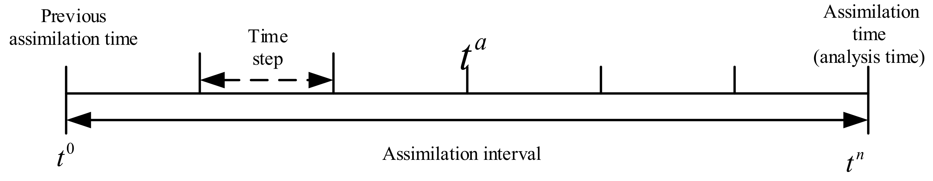
2.3. Refining Statistical Observation and Localization Scheme

The calculation of statistical observations for LEWPF-Sobs-old has been described in Section 2.2. For dealing with historical reanalysis data, the previous treatment was to calculate the mean value directly on the reanalysis data. Statistical observations can effectively avoid bias in the reanalysis data by calculating the mean, but the method disregards the correlation of the reanalysis data in the time series. In order to address this problem, we refined the previous statistical observation method by adding the time distribution of reanalysis observations to the calculation of statistical observations. The reanalysis data used in statistical observations are generally selected to correspond to the data at the observation location and these reanalysis data may be one month ago or one year ago.

Therefore, we set weights for statistical observations based on the time series distribution of the reanalysis data to calculate the mean value. It is guaranteed that data closer to the observation time will get better weights, while the more distant the time is, the smaller the weights will be. The time series distribution of the historical reanalysis data of the target observation location is shown in Figure 3. We assume the same time interval (t¹…t⁴) for reanalysis data and the $y^{t^k}$ denotes the target observation at assimilation moment t^k. The term $y_r^{t_r}$ is the reanalysis data for different historical moments t_r. The term t_r1(t³) denotes the closest reanalysis data moment to the assimilation moment t^k, while t_r4 denotes the farthest moment.

If only the reanalysis data are available at moment t_r1, the statistical observation $y_s=y_r^{t_{r1}}$. The statistical observation for any reanalysis moment $t_{rb}$ can be expressed as:

$$y_s^{t_{rb}}=\left(\frac{t_{rb}}{{\displaystyle {\sum }_{m=1}^b{t}_{rm}}}\right)\ast y_r^{t_{r1}}+\left(\frac{t_{r\left(b-1\right)}}{{\displaystyle {\sum }_{m=1}^b{t}_{rm}}}\right)\ast y_r^{t_{r2}}+\cdots +\left(\frac{t_{r1}}{{\displaystyle {\sum }_{m=1}^b{t}_{rm}}}\right)\ast y_r^{t_{rb}}$$

(19)

The term $y_s^{t_{rb}}$ represents the same meaning as $y_s^{t^b}$ given in Equation (16), indicating a statistical observation calculated based on reanalysis data. Taking $y_s^{t_{rb}}$ into Equations (17) and (18), the statistical observations calculated according to the Equation (19) can be used to determine the weights and update the particles by the proposal density.

Due to the increased complexity of the model, the calculation for the localization parameters of this algorithm also needs further refinement. Due to the simplicity of the Lorenz96 model, the particles that require localization adjustment are selected only according to the position of the state. Since the state distribution is more complex in the intermediate coupled model, the localization scheme needs to consider the spurious correlation between far points due to the lack of ensemble members. The covariance localization is used in this study, which uses a continuous function whose value is inversely proportional to the distance from the observation point to generate a multiplicative factor for the state increment:

$$\begin{array}{cc}\hfill & l_{i,j}=\Psi \left(d_{i,j},c\right)\hfill \\ \hfill & \begin{array}{cc}& =\left\{\begin{array}{c}-\frac{1}{4}{\left(\frac{d_{i,j}}{c}\right)}^5+\frac{1}{2}{\left(\frac{d_{i,j}}{c}\right)}^4+\frac{5}{8}{\left(\frac{d_{i,j}}{c}\right)}^3-\frac{5}{3}{\left(\frac{d_{i,j}}{c}\right)}^2+1\begin{array}{cc}& 0\le d_{i,j}\le c\end{array}\\ \frac{1}{12}{\left(\frac{d_{i,j}}{c}\right)}^5-\frac{1}{2}{\left(\frac{d_{i,j}}{c}\right)}^4+\frac{5}{8}{\left(\frac{d_{i,j}}{c}\right)}^3+\frac{5}{3}{\left(\frac{d_{i,j}}{c}\right)}^2-5\left(\frac{d_{i,j}}{c}\right)+1\begin{array}{cc}& c\le d_{i,j}<2c\end{array}\\ 0\begin{array}{ccc}& & d_{i,j}\ge 2c\end{array}\end{array}\right.\end{array}\hfill \end{array}$$

(20)

where d_i,j represents the distance between the observation $y_i^{t_n}$ and the positions of the model grid $x_j$. The parameter c is related to the decorrelation length. The $\Psi$ in Equation (20) is referred to as the Gaspri–Cohn (GC) function [25,26].

The localization scheme which used in the LEWPF-Sobs is designed to better handle sparsely distributed observations. The previous algorithm was studied in the Lorenz96 and from the results it can be seen that LEWPF-Sobs has some effect for sparse observation [15]. However, the case of sparse observations can be more complicated for complex gridding models, so we further improve the application of the LEWPF-Sobs localization scheme based on the previous method. Since the PF results are closely related to the observation, it is still difficult to obtain accurate particle adjustment using the localization scheme when the observations are significantly reduced. In the improved LEWPF-Sobs we use historical reanalysis data to calculate the proposed density with the aim of guiding the particles closer to the observation. Therefore, we refer to the significance of the proposal density and for sparse observation distributions we add the statistical observation proposal density to the localization scheme at the moment of assimilation. In the case of particles with no available observations in the adjustment radius at assimilation time, the proposal density is first calculated using reanalysis of historical data to fine-tune the particles to make the particles close to historical observations, and then the particles are further adjusted based on actual observations using a localization scheme.

In conclusion, the steps for assimilation using LEWPF-Sobs are as follows (assuming that the assimilation moment is tⁿ and the corresponding actual observation is $y_i^{t_n}$).

(1)

Before the moment of assimilation tⁿ. Use the statistical historical reanalysis observation $y_s^{t_{rb}}$ and Equation (19) to determine the statistical observation which used in the proposal density. Using the Equations (17) and (18) to determine the proposal density’s weights ω_i and update particles.

(2)

In the moment of assimilation tⁿ. Based on the proposal density weighs and use Equations (13)–(15) to calculate the final models states ${\left(x_i^{t^n}\right)}_{eq}$ which correspond to the observation position $y_i^{t^n}$.

(3)

In the moment of assimilation tⁿ. The particles ${\left(x_i^{t^n}\right)}_c$ without observations in the radius of influence c. The historical reanalysis data of ${\left(y_r^{t_{ra}}\right)}_c$ is the observation of the corresponding position of these particles at history moment t_ra and using them to adjust the particles ${\left(x_i^{t^n}\right)}_c$ close to the historical observations according to Equation (11) to obtain the adjusted particles ${\left(x_i^{t^n}\right)}_c^{y_r}$.

(4)

Assimilate moment tⁿ application localization schemes. Using the ${\left(x_i^{t^n}\right)}_{eq}$ and Equation (1) calculate the weight of particles around the observation based on a given observation and get the resampling indices k₁,k₂,…,k_Ne and the particles are shown as $x_{k_m}$;

(5)

In the moment of assimilation tⁿ according to the observation $y_i^{t_n}$. We refer to the localization scheme state update equations (3)–(6) and (20) of LPF. Combine the particles ${\left(x_i^{t^n}\right)}_c^{y_r}$ and resampled particles $x_{k_m}$ using the formula to update the particles within the localization radius c.

3. Cycling Data Assimilation Experiments Set Up

3.1. An Intermediate Atmosphere-Ocean-Land Coupled Model

To investigate the potential of the LEWPF-Sobs as a data assimilation algorithm for the geophysical dependence of observing systems and eliminate the computational intricacy of CGCM, an intermediate atmosphere-ocean-land coupled model [27] is used. In this study, an equation is used to represent the nonlinearity of atmosphere. The atmosphere is coupled with a 1.5-layer “baroclinic” ocean and based on the stream-function. The simple land model which the temperature is driven by the atmosphere-land fluxes. These model components adopt 96 × 48 grid points and forward points using the leapfrog time stepping method [28]. The atmosphere which is include a global pressure model and atmospheric temperature based on the equation:

$$\frac{\partial q}{\partial t}+J\left(\psi ,q\right)=\left\{\begin{array}{c}\lambda \left(T_s-\mu \psi \right)\begin{array}{cc}& ocean\end{array}\\ \lambda \left(T_l-\mu \psi \right)\begin{array}{cc}& land\end{array}\end{array}\right.$$

(21)

where $=\beta y+{\nabla }^2\psi , \beta =df/dy$, f is the Coriolis parameter, y represents the northward meridional distance from the equator, ψ represents the geostrophic atmosphere stream-function, T_S and T_L denote the sea surface temperature (SST) and land surface temperature (LST), respectively.

The ocean consists of a 1.5-layer with a slab mixed layer [29] and the stream functions are given by:

$$\left\{\begin{array}{c}\frac{\partial }{\partial t}\left(-\frac{{\phi }^2}{L_0^2}\right)+\beta \frac{\partial }{\partial x}\phi =\gamma {\nabla }^2\psi -K_q{\nabla }^2\phi \hfill \\ \begin{array}{l}\frac{\partial }{\partial t}{T}_s+\mu \frac{\partial T_s}{\partial x}+v\frac{\partial T_s}{\partial y}-K_h\psi =-K_T{T}_s\hfill \\ +A_T{\nabla }^2{T}_s+s\left(\tau ,t\right)+C_o\left(T_s-\mu \psi \right)\end{array}\hfill \end{array}\right.$$

(22)

The $\phi$ is the ocean steam-function; $L_0^2=g{h}_0/f^2$, is the oceanic deformation radius; K_h = K_T × k × f/g’ [30] represents the strength of upwelling, and the term s(τ,t) = K_T × s₀(τ) × [1 − (τ/4500 + 1/200) × cos(2π(t − 15)/360] is the solar forcing which used to represent the seasonal cycle, where $s_0$ represents the annual-mean solar forcing, τ denotes latitude, t is the day of the current moment. The evolution of LST is described by the linear equation which have the heat exchange with the atmosphere:

$$m\frac{\partial }{\partial t}{T}_l=-K_L{T}_L+A_L{\nabla }^2{T}_l+s\left(\tau ,t\right)+C_l\left(T_l-\mu \psi \right)$$

(23)

where m represents the ratio of heat capacity between the land and the ocean mixed layer. Default parameters values and meanings are detail described in the Wu [27] and the coupled mechanism is shown in the Figure 4.

The atmospheric component provides wind stress and heat flux to the ocean stream function as well as the sea surface temperature (land surface temperature), respectively, while the forcing of the sea surface temperature consists of three items: the upwelling effect of the subsurface layer, the heat flux from the atmosphere into the ocean, and solar radiation, and the forcing of the land surface temperature is forced by atmospheric heat fluxes to the land surface and solar radiation [27].

The coupling of the model is mainly reflected in physical phenomena related to flux exchange, which include the solar radiation, sensible heat flux and latent heat flux. The T_a use the sensible heat flux and the long wave radiation which are vented by the atmosphere to affect T_S and T_L l are these the same as T_S and T_L from before? Be consistent in symbols.

3.2. Simulation Experiments Setup

To examine the possibility of the improved LEWPF-Sobs used in the geophysical models, we use this method for the intermediate coupled model. This section cycling data assimilation experiments are designed to compare the characters of the LEWPF-Sobs with the LPF, the classical LEWPF-Sobs (LEWPF-Sobs-old) and the localized weighted ensemble Kalman filter (LWEnKF). The LWEnKF is presented by the Chen [24] and this algorithm is a nonlinear filter than combines the advantage of the particle filter and the ensemble Kalman filter. The main reason for selecting this method as a comparison method is that it is a hybrid method of particle filter and it also refers to the localization scheme of LPF, so it can better compare and analyze the assimilation characteristics of LEWPF-Sobs.

The experiments are divided into two parts; the first part uses standard observations to verify the effect of statistical observations based on time series on the assimilation results. The results of the experiment are presented by spatial distribution and RMSE histogram. The spatial distribution describes the adjustment of the method for all grid point position states. The annual average RMSE histogram is used to describe the deviation of the model state from the truth under different experimental conditions. As previously described LWEnKF uses the localization scheme of LPF [24] and the results are significantly better than LPF, Therefore, LWEnKF was chosen instead of LPF in the experiments of spatial distribution to compare with LEWPF-Sobs and LEWPF-Sobs-old. The second part of the experiments investigate the effect of the localization scheme of the improved LEWPF-Sobs on the assimilation results under sparse observations. Because this experiments choose the coupled model as the background therefore this experiment is divided into three parts, firstly assuming the lack of observations for T_a and T_s, respectively, and finally assuming the lack of observations for both T_a and T_s. In this part of the experiment we still choose spatial distribution and RMSE histogram to illustrate the experimental results. The different methods used under different experimental conditions and the description of the experimental results are given in

Table 1. The experimental schedule.

	Standard Observation		Spare Observation
	Spatial Distribution	RMSE Histogram	Spatial Distribution	RMSE Histogram
LEWPF-Sobs	√	√	√	√
LEWPF-Sobs-old	√	√	√	√
LWEnKF	√	√	√	√
LPF		√		√

.

We initialize the model with the annual mean of grid model states of corresponding climatological domains [31]. The model of the Dommenget and Flöter [32] scheme was used as the true value to generate observations, and the assimilation scheme used the Thompson and Warren [33] scheme. The truth model is run from the initial conditions, climatological fields of six prognostic variables [31]. This model is run for 4 years as the spin-up circle and the assimilation adjustment is start form the 5th year and the statistical analysis of assimilation results of the 6th year.

The truth x^t is obtained from the integration of the time series after the spin-up. The observations are determined by the equation:

$$y=H\left[x^t\right]+\epsilon$$

(24)

where H is a function that maps the model truth x^t, which are based on the distribution of the observation and $\epsilon$ is the observation error with a white noise. The atmosphere T_a standard observational error is 0.5 and the T_S and T_L use the observational error 1. In the experiments, it is necessary to use historical reanalysis data to determine statistical observations which used in the proposed density to adjusted ensemble particles. The reanalysis data is determined by adding white noise to the truth of the 4th year according to the Equation (24) and it is corresponding to the full time series distribution of the model grid positions. The model integral time is for 12 h as one integral step, while corresponding sampling frequencies are one integral step (12 h for T_a), four integral steps (48 h for T_s) in this experiments. In this paper, the observations are distributed uniformly distributed of the model grids. To roughly simulate real-world scenario so this model and initial condition which have the biased information similar to the observations.

The root-mean-square-error (RMSE) as an important criterion for evaluating assimilation quality, the RMSE is defined as:

$$RMSE=\sqrt{\frac{1}{N_x}{\displaystyle \sum _{i=1}^{N_x}{\left(x_i-x_i^t\right)}^2}}$$

(25)

where the x_i is the model state with the variable i and $x_i^t$ is the truth. The RMSE method is used to evaluate the assimilation results and both experiments are performed using the same initial particles. The RMSE of the T_a variable is expressed as Ta-RMSE and the RMSE of T_s is expressed as Ts-RMSE according to Equation (25).

Before the experiment, first confirm the start moment of statistical observation, the longest assimilation interval is 4 integration steps, so according to the time series of statistical observation distribution shown in Figure 2 and Figure 3, the RMSE results corresponding to the two statistical observation calculation methods are shown in the Figure 5. In the figure we uniformly choose t_rb as the horizontal coordinate, and the relationship between the two method times is t_r1 = (t^a = 3) = t³.

As it can be seen from the Figure 5, the improved method for calculating statistical observations which is given in Section 2.3 is slightly reduced from the previous method about the RMSE of T_a and T_s. It can be seen that the incorporation of reanalysis data in the time dimension into the computation of statistical observations can significantly improve the forecast accuracy. T_a and T_s can obtain smaller RMSE when t_rb = 3, which means that the maximum number of reanalysis data is applied to calculate the statistical observation proposal density in the assimilation interval. These data ensure that the particles are guided close to the observation at each moment before assimilation finally guarantee the optimal final assimilation result. The RMSE of both T_a and T_s converge to the observation error covariance when (t_rb = 0) = (t^a = 4) = t⁴. The reason is that if t_rb = 0, it means that no statistical observation introduces the proposal density and only the observation at the moment of assimilation is considered. In order to ensure the accuracy of assimilation results in subsequent experiments, t_rb = 3 was chosen for all subsequent experiments.

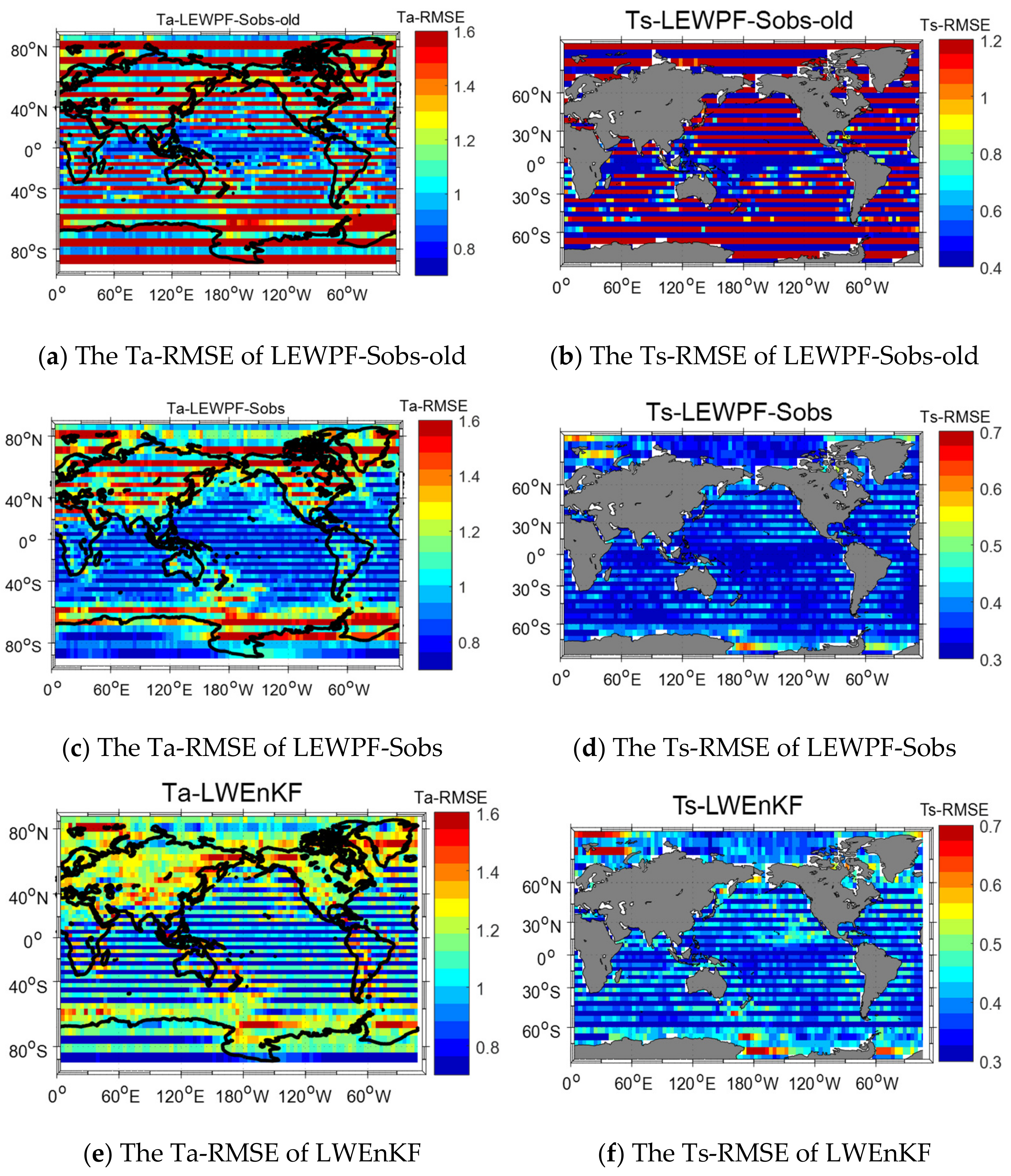
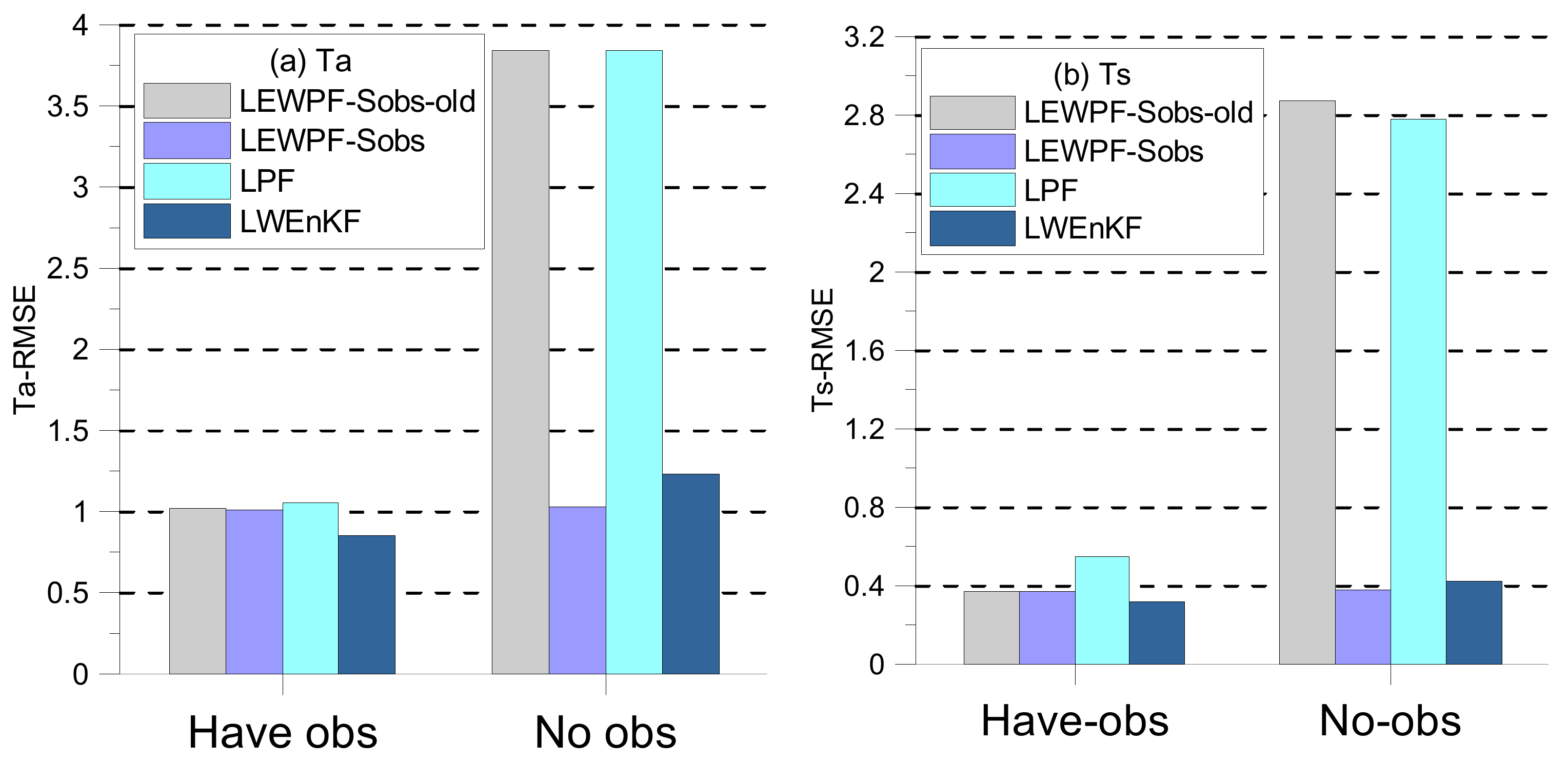
4. The Numerical Experimental Results

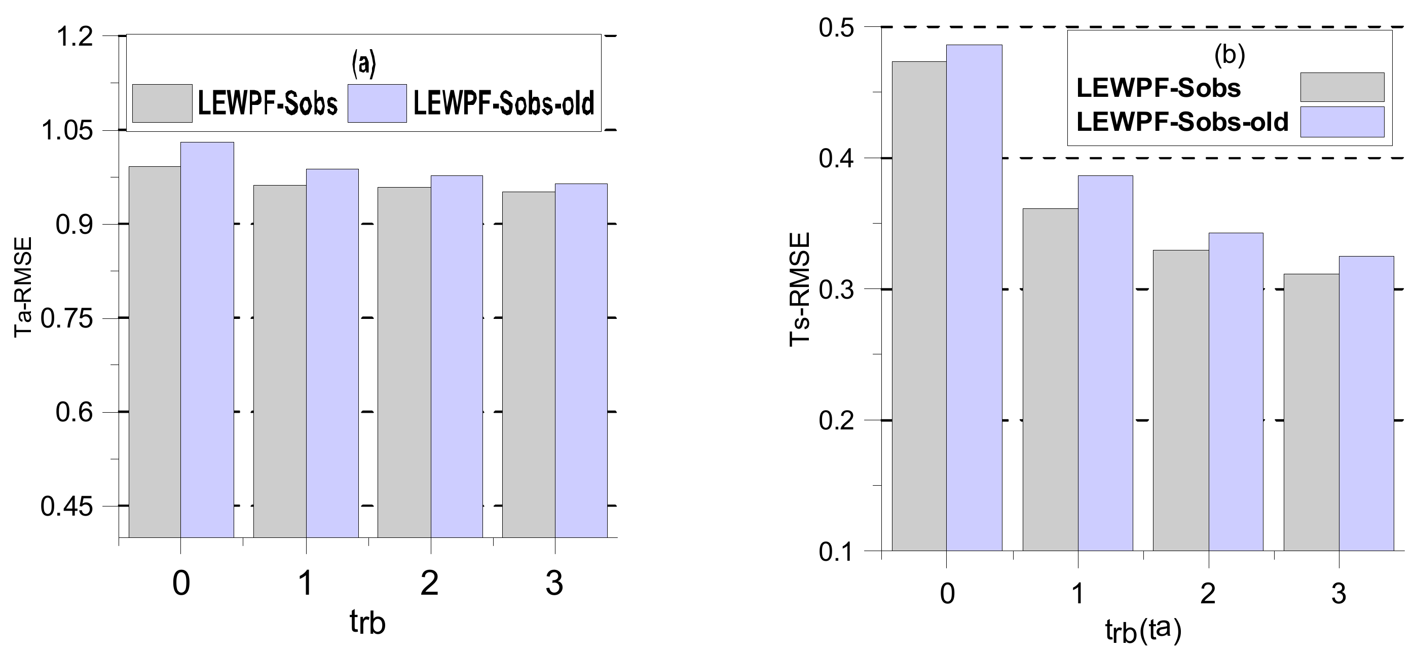
4.1. Standard Observation Distribution Experiment

This part tests the LEWPF-Sobs is a situation which uses Equation (24) to determine the global standard observation distribution and the observations have uncorrelated Gaussian errors with standard errors of different variables (T_a and T_s). The experiment is designed to verify whether the LEWPF-Sobs can get reliable filtering results for realistic geophysical systems. The final statistics are calculated based on the T_a and T_s with three methods in the assimilation cycle. We use the domain average of RMSE and average ensemble Spread for all variables to evaluate the assimilation effect of these methods. Thus the annual RMSE for the different methods in this coupled model is shown in Figure 6.

In order to comprehensively analyze the assimilation results of the grid points, Figure 6 shows the geographic-dependent distribution of annual RMSE of T_a and T_s about the LEWPF-Sobs-old (panel a and b), LWEnKF (panel c and d) and LEWPF-Sobs (panel e and f). The three algorithms of atmospheric temperature use the similar color calibration scale, it can be seen that the atmospheric of the LEWPF-Sobs has the better RMSE which is maintained at about 0.8, while the RMSE of the LEWPF-Sobs which use the improve statistical observation is little better than the LEWPF-Sobs-old. The LEWPF-Sobs also has the lowest RMSE about the T_s which is stable around 0.35. The LWEnKF and LEWPF-Sobs have similar results about the T_a and T_s. The RMSE of LWEnKF is slightly higher than LEWPF-Sobs and the results of the T_a are better than the LEWPF-Sobs in some regions. It has more stabled results about the T_s. However, based on the above results, the accuracy and stability of LEWPF-Sobs is superior to the other methods.

According to the geographic-dependent distribution results, we further analyze the use of these algorithms to calculate the posterior particles. Since the LEWPF-Sobs which use the improved statistical observations, this method was incorporated into the subsequent experiments in order to further investigate the effect of statistical observations on the assimilation results. In practice, it is difficult to guarantee that all observation are Gaussian. For non-Gaussian observations, the advantage of the PF is flexibility to choose the likelihood for calculating weights to accommodate non-Gaussian errors. The observations are generated by the Equation (24) use Gaussian errors in the previous experiments. For this experiment, we use H(x) = |x| and H(x) = ln(|x|) to replace the Gaussian observation error to further refine the subsequent experiments. Figure 7 shows the average RMSE for annual average of all variables with different algorithms, respectively.

Since the localization schemes of the LEWPF and LWEnKF both refer to the LPF, the LPF is presented as a comparison method in this part of the experiment. Figure 7a illustrates the annual average RMSE of atmospheric temperature with different non-Gaussian operators. The LEWPF-Sobs-old and LEWPF-Sobs give similar results and the LEWPF-Sobs is a little smaller than the previous algorithm when useing different observational operators. The LPF maintained better assimilation results, but the RMSE was slightly higher than that of LEWPF-Sobs. It can also be seen from the experimental results that the RMSE of LPF is closer to the observation error, the reason is the LPF update the particles only based on the observation so the forecast error approximate to the observation. The LWEnKF and LEWPF-Sobs have the similar results which are better than the other algorithms. Moreover, when using non-Gaussian operators, its results are slightly worse than LEWPF-Sobs. The RMSE of ocean temperature are given in the Figure 7b. It can be seen that T_s gives similar results to T_a. The improved LEWPF-Sobs obtained better results for different non-Gaussian observation operators and the final results are more accurate than those of the other algorithms. The experimental results demonstrate that calculating statistical observations based on time series can significantly improve the calculation results of the proposed density and increase the accuracy of assimilation results. These experiments, therefore, indicates the LEWPF-Sobs can provide accurate results in a wide range of applications.

The annual mean of the RMSE and Spread of the different algorithms used in experiments with different observation distribution are shown in the

Table 2. The LEWPF-Sobs, LPF, LWEnKF and LEWPF-Sobs-old annual averaged RMSE and Spread of particles for experiment.

	H(x) = x		H(x) = |x|		H(x) = ln(|x|)
	RMSE	Spread	RMSE	Spread	RMSE	Spread
Atmospheric temperature (Ta)
LPF	1.024866	0.89107	1.1214	0.9105	1.24840	0.8889
LEWPF-Sobs-old	0.960692	0.30691	1.1184	0.314	1.23545	0.4399
LEWPF-Sobs	0.951810	0.32541	1.0215	0.421	1.2124	0.456
LWEnKF	1.0048	0.296	1.114	0.301	1.2254	0.412
Ocean temperature (Ts)
LPF	0.47064	0.421315	0.503	0.5031	0.58093	0.45319
LEWPF-Sobs-old	0.356783	0.357434	0.497	0.478	0.56165	0.47837
LEWPF-Sobs	0.3310	0.34756	0.4786	0.487	0.5487	0.4863
LWEnKF	0.3229	0.3341	0.4885	0.469	0.551	0.464

. The four algorithms have the similar RMSE under different Gaussian distribution observations. It also gives the LPF has better adjustment of the relationship between the RMSE and Spread and the spread of LEWPF-Sobs has smaller results which is reasonable because of the proposal density was used to adjust the particle spacing and make the particles have similar results. For the variable T_a the RMSE of the improved LEWPF-Sobs reduces 2% compared to the traditional LEWPF-Sobs while the T_s variable reduces by 7.3%.

4.2. Sparse Observational Distribution Experiments

In the actual situation, it is difficult to obtain the global observations which used in the data assimilation and lack of accurate observation at many locations. Therefore, the second part of the experiments design sparse observation distributions to study the potential of the LEWPF-Sobs for subsequent practical applications. The model components adopt 96 × 48 grid points and removes half of the observations from these points to simulate the actual lack of observations in some areas. Because this model is a coupled model, in order to fully analyze the experimental results, for the experiments with sparse observations, it is first assumed that the atmospheric temperature (T_a) lacks observations. In these experiments the final statistics are also use the average of RMSE for T_a and T_s as the evaluation criterion. Therefore the annual RMSE about the T_a and T_s for the different algorithms are shown in Figure 8.

Figure 8 illustrates the geographic-dependent distribution of annual average RMSE with different algorithms when T_a use the sparse observations. It can be clearly seen that the RMSE is significantly higher at the location where the observation is missing and the LEWPF-Sobs (panel c) and LWEnKF (panel e) with observed locations can obtain better RMSE, while for the part lacking observations both methods have similar results but the LWEnKF is better than LEWPF-Sobs in some regions. The LEWPF-Sobs is significantly improved by adding the statistical observation proposal density to the localization scheme. As seen in panel c, most of the regions can maintain small RMSE, while only sporadic regions have some deviation. It can be seen that the results of LEWPF-Sobs are more stable due to the application of the proposal density to the adjustment of sparsely observed particles. Because the experiment uses the coupled model, the atmospheric bias will have an effect on the ocean. From panels b, d and f, we can see that the LEWPF-Sobs-old have large biases in the most of regions. The reason is that the lack of observation of T_a increases the bias of assimilation results in some regions and thus affects the assimilation results of T_s. However, it can be seen from the results that the LEWPF-Sobs is better than LWEnKF. Although the overall results of LWEnKF are more stable and the LEWPF-Sobs has the better overall results due to the more accurate assimilation results of T_a and therefore less impact on T_s.

Similarly Figure 8 and Figure 9 illustrate the geographic-dependent distribution of annual average RMSE of different algorithms when T_s use the sparse observations. The panel (a,c,e) shows the assimilation results of the LEWPF-Sobs for T_a are significantly better than the other algorithms. However, the absence of T_s observations in the coupled model makes the RMSE of LEWPF-Sobs-old is significantly changed, the error is smaller in the part with observation, while the deviation is larger in the part without observation. The results of LEWPF-Sobs and LWEnKF are more similar, but the LEWPF-Sobs are more stable and its RMSE is smaller. And because LEWPF-Sobs (panel d) has better results for T_s, thus improving the assimilation results of T_a in this coupled model. Based on the above two parts of experimental results, it can be seen that the refined LEWPF-Sobs has a significant improvement for the assimilation of sparse observations and this algorithm is more suitable for the coupled model and reduces the influence of sparse observations on the assimilation results.

In order to analyze the effect of sparse observations more comprehensively, we assume that both T_a and T_s are lacking half of the observations, then the assimilation results of the three methods are shown Figure 10. The RMSE of T_a and T_s are larger than in the previous experiments (Figure 8 and Figure 9) due to the lack of partial observations. Because the previous experiments assumed that only one variable lacked observations, this variable could be adjusted to reduce the bias by assimilating other variables based on the coupled model. However, in this part of the experiments, because both variables are missing observations and therefore the adjustment of the variables relies only on the assimilation method, it is possible to better compare which method is more suitable for the assimilation requirements of sparse observations.

From Figure 10, it can be seen that LEWPF-Sobs (panels c and d) consistently has the best assimilation results and the RMSE is significantly smaller than with the other two methods. The results of LWEnKF (panels e and f) are slightly better than the LEWPF-Sobs-old (panel a and b). It can be seen from the figures, LEWPF-Sobs and LWEnKF have similar results, but the RMSE of LWEnKF is smaller in some regions of the T_a and the assimilation results of LEWPF-Sobs are better than LWEnKF for the variables T_s. The results of LEWFP-Sobs-old are worse than the other algorithms when the area lack of the observations and the main reason for this result is that the PF relies on observations for assimilation, and the bias of the assimilation results will be increased when there are fewer observations available. The LEWPF-Sobs (panels b and d), which improved by adding the statistical observation proposal density to the localization scheme, gives the best assimilation results for the T_s variables, and although bias still exists in some regions of the ta variables, the RMSE of T_a is maintained at a small value overall.

For further research the effect of the localization scheme on the lack of observed location particles, we select all grid points of T_a and T_s where observations are missing to investigate the ensemble states based on LEWPF-Sobs-old (gray), LEWPF-Sobs (pastel blue), LPF (ice blue) and LWEnKF (desert blue)which are shown in the Figure 11. Panel (a) and (b) gives the results of the RMSE of the variable T_a and T_s based on different algorithms with different observation situations. The results of the four methods are closer when observations are available, while the most significant increase in RMSE can be seen for LPF and LEWPF-Sobs-old when observations are missing. The LEWPF-Sobs and LWEnKF, consistently provide better assimilation results for different observation distributions and the results of LWEnKF are slightly better than LEWPF-Sobs for T_a, while the assimilation results of LEWPF-Sobs are better for T_s variables. It can be seen from Figure 11 that the improved LEWPF-Sobs incorporates statistical observations into the localization scheme, which can effectively improve the assimilation results of sparse observations and reduce the bias between ensemble particles. From the experimental results, it can be seen that the RMSE of the variable T_a which have observation is reduced by 2% for the improved LEWPF-Sobs compared to the LEWPF-Sobs-old while the T_s variable is reduced by 8%, which is similar to the standard observation. However, under the sparse observation condition, the RMSE of the improved LEWPF-Sobs for the variable T_a is reduced by 73.2% compared to the traditional method, while for the variable T_s it is reduced by 86.8%.

5. Discussion and Conclusions

This paper describes the application of the improved LEWPF-Sobs for data assimilation in the intermediate coupled model while avoiding the limitations of traditional particle filters. In order to better apply the coupled model based on the previous method, we propose to calculate statistical observations based on time series distribution weights that take into account the distribution of the historical reanalysis data on the time scale. In order to improve the application of the localization scheme with sparse observations, it is proposed to introduce statistical observations into the localization scheme, which is adjusted for sparse observations.

In this paper, we analyzed the statistical observations based on time series distribution of the historical reanalysis data and improved localization scheme as used in the LEWPF-Sobs to improve the ability to perform the grid coupled model. According to the experimental results, the LEWPF-Sobs always maintains the minimum T_a and T_s RMSE compared to LEWPF-Sobs-old and LWEnKF. The spatial distribution of annual average RMSE also shows the LEWPF-Sobs when use the improved statistical observations give more accurate assimilation results than the previous algorithm. When non-Gaussian observations are used in these experiments, the LWEnKF and LEWPF-Sobs have similar results, the main reason being that the PF have an obvious advantage when dealing with nonlinear and non-Gaussian problems and the LEWPF-Sobs results are more stable. To further investigate the effect of the improved localization scheme which used in the LEWPF-Sobs, the algorithm is tested in the experiments which remove half of observations. The LEWPF-Sobs can adjust the ensemble particles towards the truth corresponding to the lack of observation position through the localization scheme. The comparison of the RMSE under different observation conditions shows that the improved LEWPF -Sobs has a better adjustment of particles not only in the observed position, but also in the absence of observation positions. The improved localization scheme uses the proposal density which are calculated by the reanalysis data making the results better than the previously method, therefore the final results of the LEWPF-Sobs is more accurate.

Based on the above experimental results, it can be seen that the statistical observation calculation method based on time series distribution can effectively improve the assimilation results to increase the accuracy compared with the previous method which only calculate the mean of the historical reanalysis data. The RMSEs of variables T_a and T_s are reduced by 2% and 8%, respectively. For the improved localization scheme, the assimilation results of the localization scheme are improved due to the use of statistical observation proposal density adjusted for unobserved positional particles which are based on historical reanalysis data. Therefore this method has a good adjustment for sparse observations and improves the assimilation accuracy. The location of the missing observation, the improved method reduces the RMSE of the variables T_a and T_s by 73.2% and 86.8%, respectively. It can be seen that the LEWPF-Sobs can be better applied to the coupled model, while the variables for which no observations are available can be better adjusted through the localization scheme. It can be seen that the assimilation results of the improved LEWPF-Sobs is better than tradition algorithms.

From the experimental results of sparse observations, it can be seen that the improved localization scheme still has an atmospheric temperature bias, and further improvement of the localization method will be necessary in the subsequent research. For the research of statistical observations, the subsequent research will introduce intelligent methods such as machine learning to determine the observations instead of the reanalysis data, which can further improve the reliability of the observation while avoiding the error of the statistical observation. Further study of LEWPF-Sobs assimilation systems is suitable for mesoscale models which has practical implications.

References

1. Evensen, G. Sequential data assimilation with a nonlinear quasi-geostrophic model using Monte Carlo methods to forecast error statistics. J. Geophys. Res. Ocean. 1994, 99, 10143–10162. [Google Scholar] [CrossRef]
2. Nichols, N.K. Data Assimilation: Aims and Basic Concepts. In Data Assimilation for the Earth System; Springer: Berlin/Heidelberg, Germany, 2003; pp. 9–20. [Google Scholar]
3. Evensen, G.; Leeuwen, P.V. Assimilation of Geosat Altimeter Data for the Agulhas Current using the Ensemble Kalman Filter with a Quasi-Geostrophic Model. Mon. Weather Rev. 1995, 124, 85–96. [Google Scholar] [CrossRef]
4. Jadidoleslam, N.; Mantilla, R.; Krajewski, W.F. Data Assimilation of Satellite-Based Soil Moisture into a Distributed Hydrological Model for Streamflow Predictions. Hydrology 2021, 8, 52. [Google Scholar] [CrossRef]
5. Chen, Y.; Zhang, W.; Zhu, M. A localized weighted ensemble Kalman filter for high-dimensional systems. Q. J. R. Meteorol. Soc. 2020, 146, 438–453. [Google Scholar] [CrossRef] [Green Version]
6. Wu, P.Y.; Yang, S.C.; Tsai, C.C.; Cheng, H.W. Convective-Scale Sampling Error and Its Impact on the Ensemble Radar Data Assimilation System: A Case Study of a Heavy Rainfall Event on 16 June 2008 in Taiwan. Mon. Weather Rev. 2020, 148, 3631–3652. [Google Scholar] [CrossRef]
7. Pires, C.A.; Talagrand, O.; Bocquet, M. Diagnosis and impacts of non-Gaussianity of innovations in data assimilation. Phys. D Nonlinear Phenom. 2010, 239, 1701–1717. [Google Scholar] [CrossRef] [Green Version]
8. Van Leeuwen, P.J.; Künsch, H.R.; Nerger, L.; Potthast, R.; Reich, S. Particle filters for high-dimensional geoscience applications: A review. Q. J. R. Meteorol. Soc. 2019, 145, 2335–2365. [Google Scholar] [CrossRef]
9. Van Leeuwen, P.J. Particle filtering in geophysical systems. Mon. Wather Rev. 2009, 137, 4089–4114. [Google Scholar] [CrossRef]
10. Van Leeuwen, P.J.; Cheng, Y.; Reich, S. Nonlinear Data Assimilation; Springer International Publishing: Berlin/Heidelberg, Germany, 2015. [Google Scholar]
11. Potthast, R.; Walter, A.; Rhodin, A. A localized adaptive particle filter within an operational NWP framework. Mon. Weather Rev. 2019, 147, 345–362. [Google Scholar] [CrossRef]
12. Brajard, J.; Carrassi, A.; Bocquet, M.; Bertino, L. Combining data assimilation and machine learning to infer unresolved scale parametrization. Philos. Trans. R. Soc. A 2021, 379, 20200086. [Google Scholar] [CrossRef]
13. Khan, R.S.; Bhuiyan, M.A.E. Artificial Intelligence-Based Techniques for Rainfall Estimation Integrating Multisource Precipitation Datasets. Atmosphere 2021, 12, 1239. [Google Scholar] [CrossRef]
14. van Leeuwen, P.J. Aspects of Particle Filtering in High-Dimensional Spaces. In Dynamic Data-Driven Environmental Systems Science; Springer International Publishing: Berlin/Heidelberg, Germany, 2015; pp. 251–262. [Google Scholar]
15. Zhao, Y.; Yang, S.; Jia, R.; Zhou, D.; Deng, X.; Liu, C.; Wu, X. The statistical observation localized equivalent-weights particle filter in a simple nonlinear model. Acta Oceanol. Sin. 2021. [Google Scholar] [CrossRef]
16. Poterjoy, J.; Wicker, L.; Buehner, M. Progress toward the application of a localized particle filter for numerical weather prediction. Mon. Weather Rev. 2018, 147, 1107–1126. [Google Scholar] [CrossRef]
17. Poterjoy, J. A localized particle filter for high-dimensional nonlinear systems. Mon. Weather Rev. 2016, 144, 59–76. [Google Scholar] [CrossRef]
18. Poterjoy, J.; Anderson, J.L. Efficient Assimilation of Simulated Observations in a High-Dimensional Geophysical System Using a Localized Particle Filter. Mon. Weather Rev. 2016, 144, 2007–2020. [Google Scholar] [CrossRef]
19. van Leeuwen, P.J. Nonlinear data assimilation in geosciences: An extremely efficient particle filter. Q. J. R. Meteorol. Soc. 2010, 136, 1991–1999. [Google Scholar] [CrossRef] [Green Version]
20. Poterjoy, J.; Anderson, J.L. Particle filters for high-dimensional geoscience applications: A review. Q. J. R. Meteorol. Soc. 2018, 723, 2335–2365. [Google Scholar]
21. Ades, M.; Van Leeuwen, P.J. An exploration of the equivalent weights particle filter. Q. J. R. Meteorol. Soc. 2013, 139, 820–840. [Google Scholar] [CrossRef]
22. Zhu, M.; Van Leeuwen, P.J.; Amezcua, J. Implicit equal-weights particle filter. Q. J. R. Meteorol. Soc. 2016, 142, 1904–1919. [Google Scholar] [CrossRef] [Green Version]
23. Van Leeuwen, P.J. Efficient nonlinear data-assimilation in geophysical fluid dynamics. Comput. Fluids 2011, 46, 52–58. [Google Scholar] [CrossRef] [Green Version]
24. Chen, Y.; Zhang, W.; Wang, P. An application of the localized weighted ensemble Kalman filter for ocean data assimilation. Q. J. R. Meteorol. Soc. 2020, 146, 3029–3047. [Google Scholar] [CrossRef]
25. Gaspari, G.; Cohn, S.E. Construction of correlation functions in two and three dimensions. Q. J. R. Meteorol. Soc. 1999, 125, 723–757. [Google Scholar] [CrossRef]
26. Shen, Z.; Tang, Y.; Li, X. A new formulation of vector weights in localized particle filters. Q. J. R. Meteorol. Soc. 2017, 143, 3269–3278. [Google Scholar] [CrossRef] [Green Version]
27. Wu, X.; Zhang, S.; Liu, Z.; Rosati, A.; Delworth, T.L.; Liu, Y. Impact of Geographic-Dependent Parameter Optimization on Climate Estimation and Prediction: Simulation with an Intermediate Coupled Model. Mon. Weather Rev. 2011, 140, 3956–3971. [Google Scholar] [CrossRef]
28. Robert, A. The integration of a spectral model of the atmosphere by the implicit method. In Proceedings of the WMO/IUGG Symposium on NWP, Tokyo, Japan, 26 November–4 December 1968. [Google Scholar]
29. Liu, Z. Interannual positive feedbacks in a simple extratropical air-sea coupling system. J. Atmos. Sci. 1993, 50, 3022–3028. [Google Scholar] [CrossRef] [Green Version]
30. Philander, S.G.H. Unstable air-sea interaction in the tropics. J. Atmos. 1984, 41, 604–613. [Google Scholar] [CrossRef]
31. Zhang, X.F.; Zhang, S.; Liu, Z. Parameter optimization in an intermediate coupled climate model with biased physics. J. Clim. 2015, 28, 1227–1247. [Google Scholar] [CrossRef]
32. Dommenget, D.; Flöter, J. Conceptual understanding of climate change with a globally resolved energy balance model. Clim. Dyn. 2011, 37, 2143–2165. [Google Scholar] [CrossRef]
33. Thompson, S.L.; Warren, S.G. Parameterization of outgoing infrared radiation derived from detailed radiative calculations. J. Atmos. Sci. 1982, 39, 2667–2680. [Google Scholar] [CrossRef] [Green Version]
Figure 1. Schematic showing the assimilation interval in terms of the model integration step. The term tn is the time of the future observation, ta is the start time.
Jmse 09 01153 g001
Figure 2. Schematic diagram showing the assimilation interval and the starting moment ta of statistical observations.
Jmse 09 01153 g002
Figure 3. Schematic diagram showing the historical reanalysis of data time series and the reanalysis moment trb and assimilation moment tk.
Jmse 09 01153 g003
Figure 4. Coupled mechanism.
Jmse 09 01153 g004
Figure 5. The annual average RMSE with different start moment of statistical observation trb for the LEWPF-Sobs. (a) The average RMSE of Ta. (b) As (a) but for the Ts.
Jmse 09 01153 g005
Figure 6. The spatial distribution of annual average RMSE of panel (a,c,e) the atmospheric temperature (Ta) RMSE with respect to LEWPF-Sobs-old, LWEnKF and LEWPF-Sobs. The panel (b,d,f) are similar to panel (ac) but for the ocean temperature (Ts).
Jmse 09 01153 g006
Figure 7. The annual average RMSEs of the data assimilation with LEWPF-Sobs, LPF, LEWPF-Sobs-old and LWEnKF with different observation operators. (a) The average RMSE of Ta with different algorithms. (b) As (a) but for the Ts.
Jmse 09 01153 g007
Figure 8. The spatial distribution of annual average RMSE of panel (a,c,e) the atmospheric temperature (Ta) use the spare observations and the RMSE with respect to LEWPF-Sobs-old, LEWPF-Sobs and LWEnKF. The panel (b,d,f) are similar to panel (a,c,e) but for the ocean temperature (Ts) with standard observations.
Jmse 09 01153 g008aJmse 09 01153 g008b
Figure 9. The spatial distribution of annual average RMSE of panel (a,c,e) the atmospheric temperature (Ta) and the RMSE with respect to LEWPF-Sobs-old, LWEnKF and LEWPF-Sobs. The panel (b,d,f) are similar to panel (a,c,e) but for the ocean temperature (Ts) use the spare observations.
Jmse 09 01153 g009
Figure 10. The spatial distribution of annual average RMSE of panel (a,c,e) the atmospheric temperature (Ta) use the spare observations and the RMSE with respect to LEWPF-Sobs-old, LEWPF-Sobs and LWEnKF. The panel (b,d,f) are similar to panel (a,c,e) but for the ocean temperature (Ts) use the sparse observations.
Jmse 09 01153 g010
Figure 11. The RMSE histogram of the grid points with different observation situations. The RMSE of the variable Ta based on the LEWPF-Sobs-old (gray), LEWPF-Sobs (pastel blue), LPF (ice blue) and LWEnKF (desert blue). The panel (b) is similar to the (a) but for the variable Ts.
Jmse 09 01153 g011