
Modelling the Past and Future Evolution of Tidal Sand Waves


Abstract
1. Introduction
2. Materials and Methods
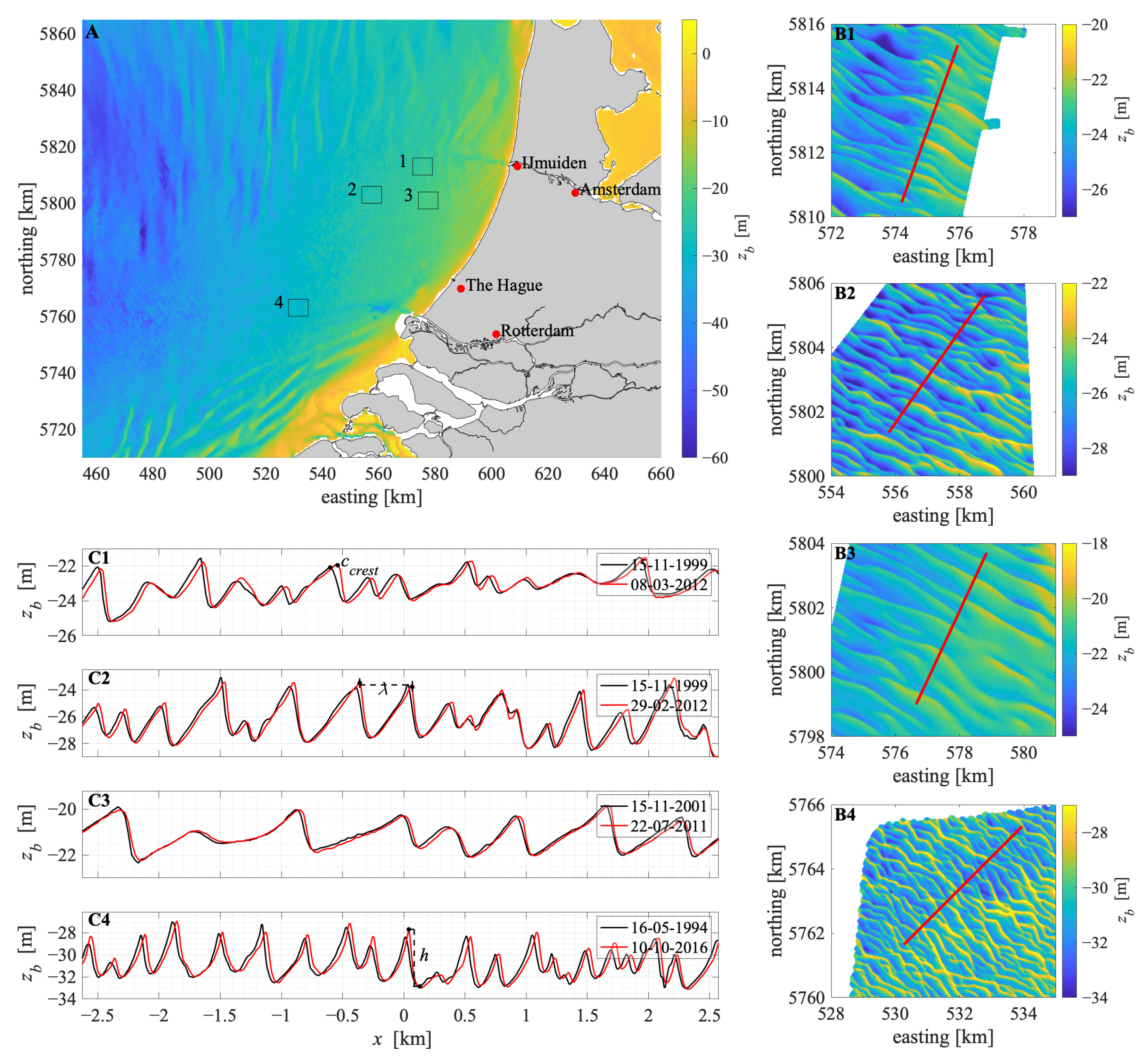
2.1. Study Sites
2.2. Model Description
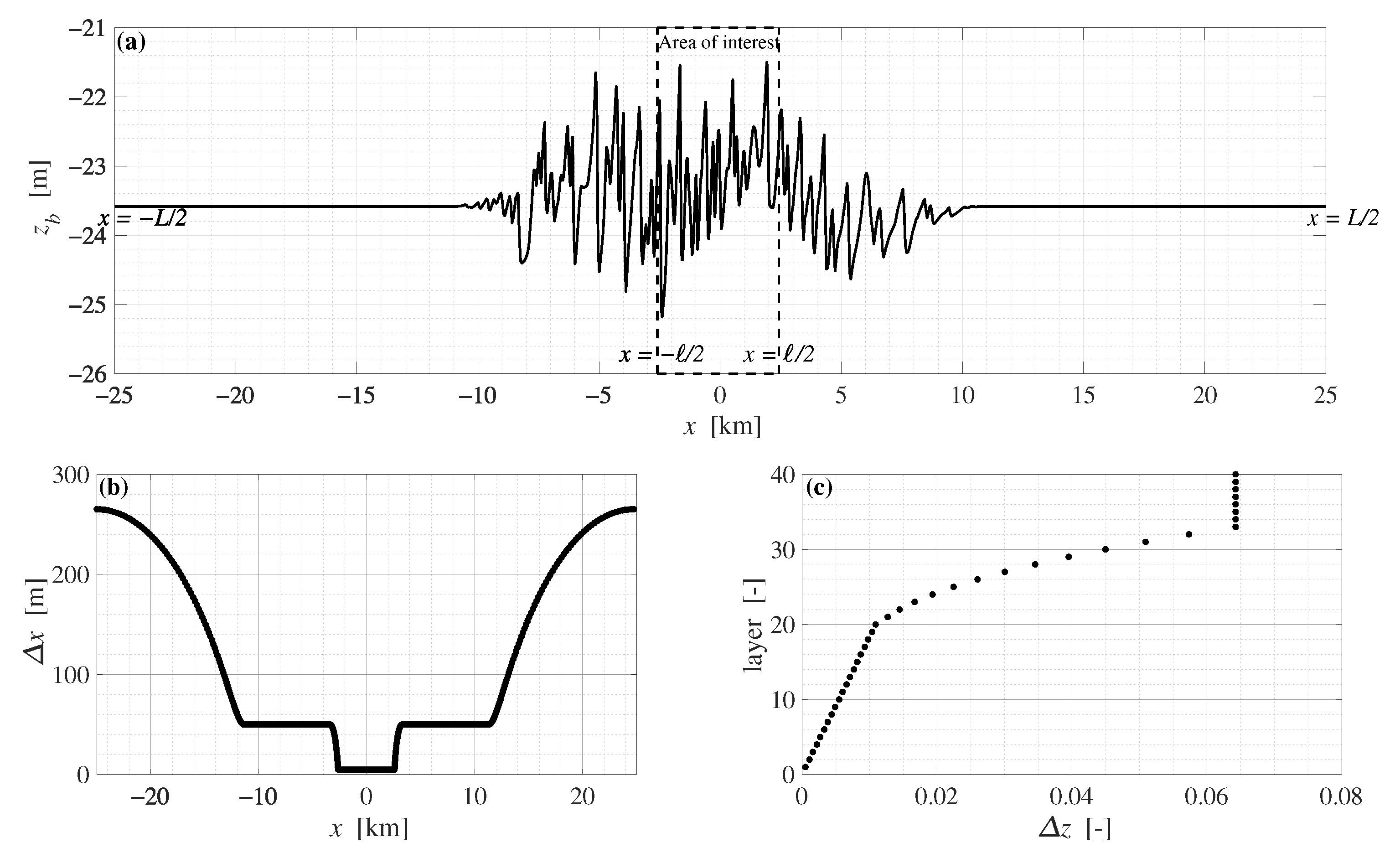
2.3. Model Configuration
2.4. Design of Experiments
2.5. Analysis of Model Output
3. Results
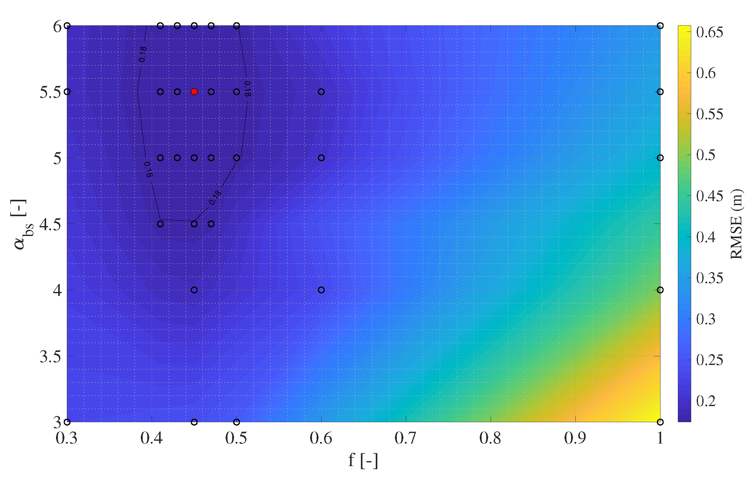
3.1. Calibration
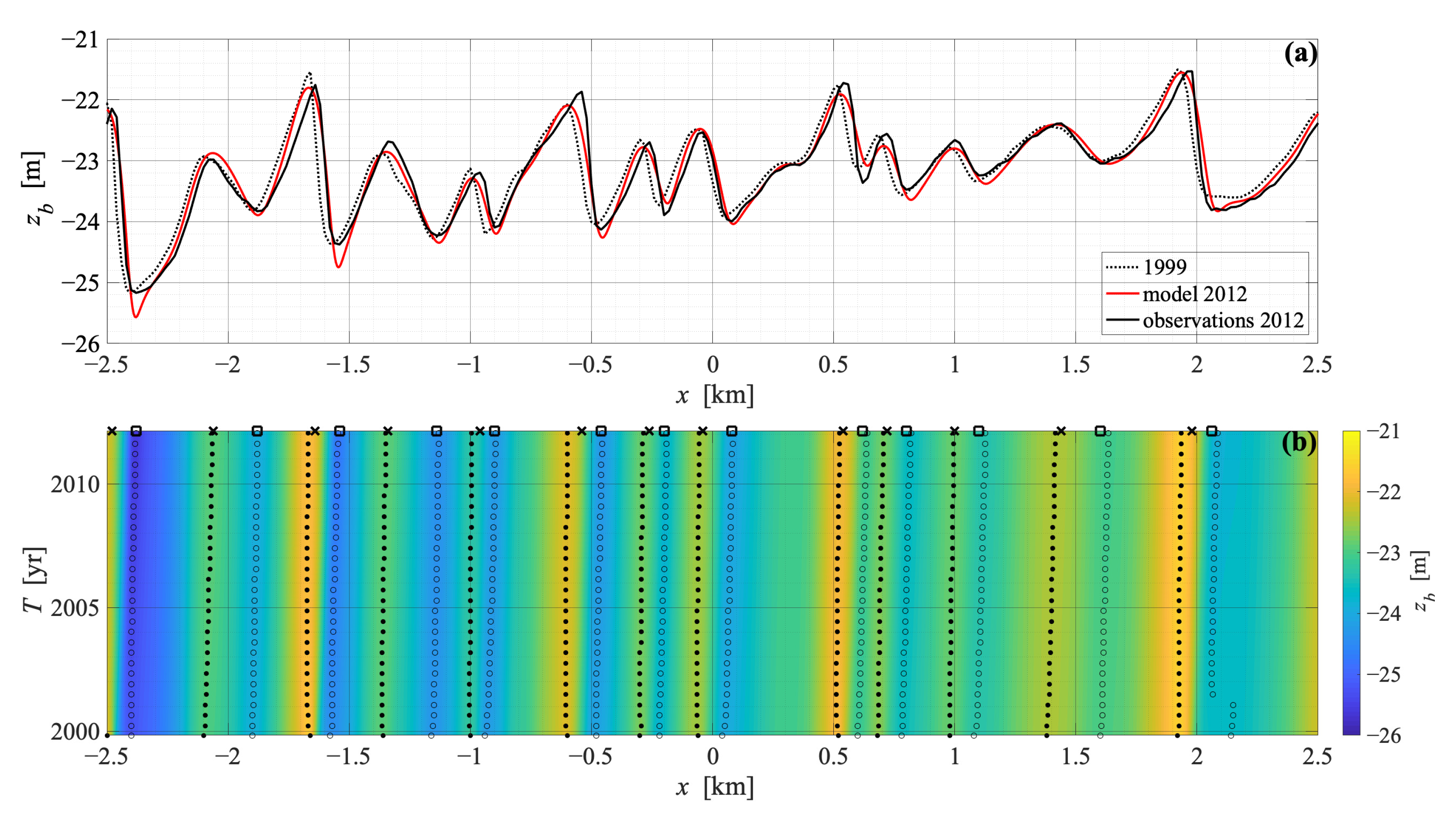
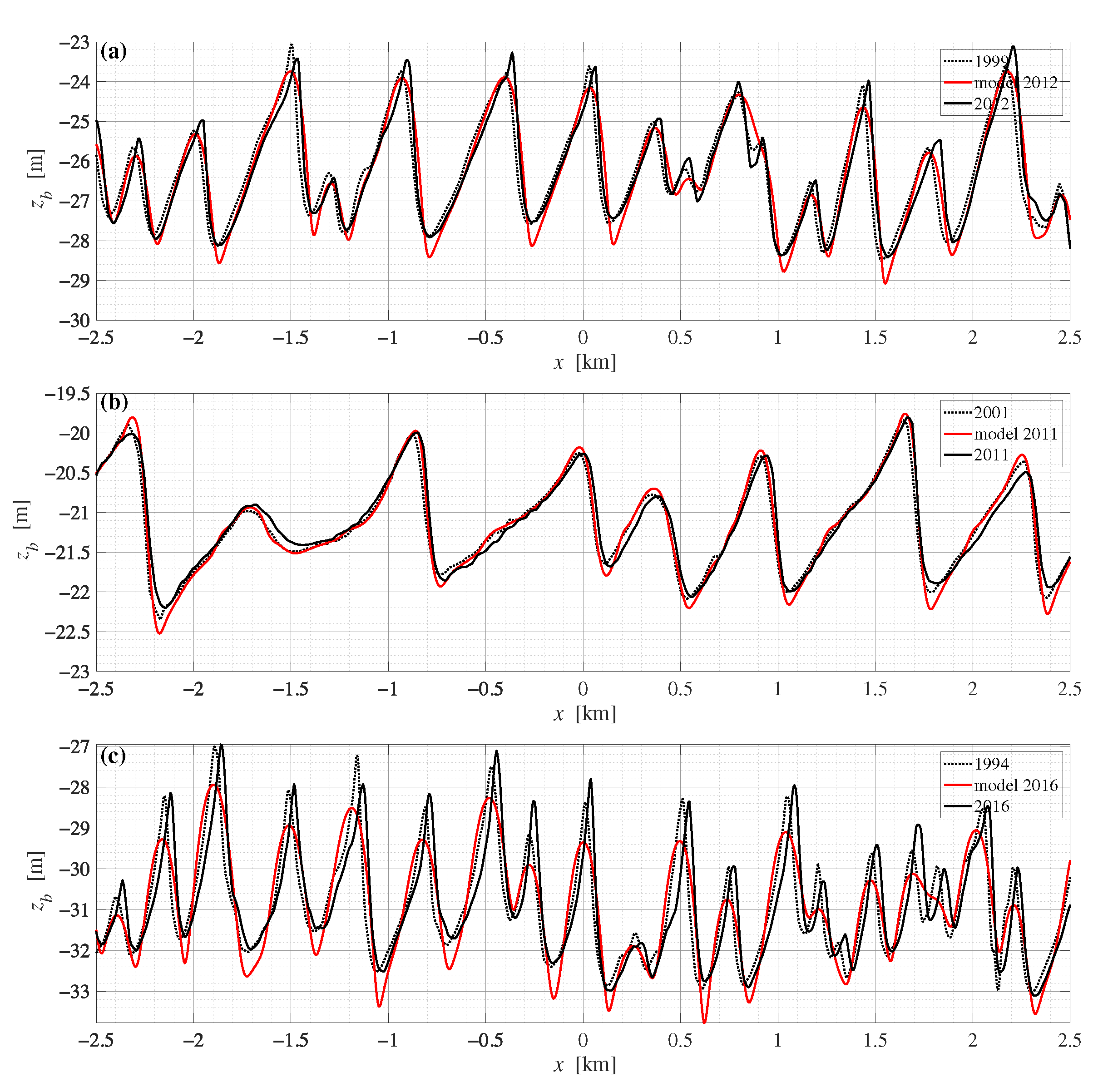
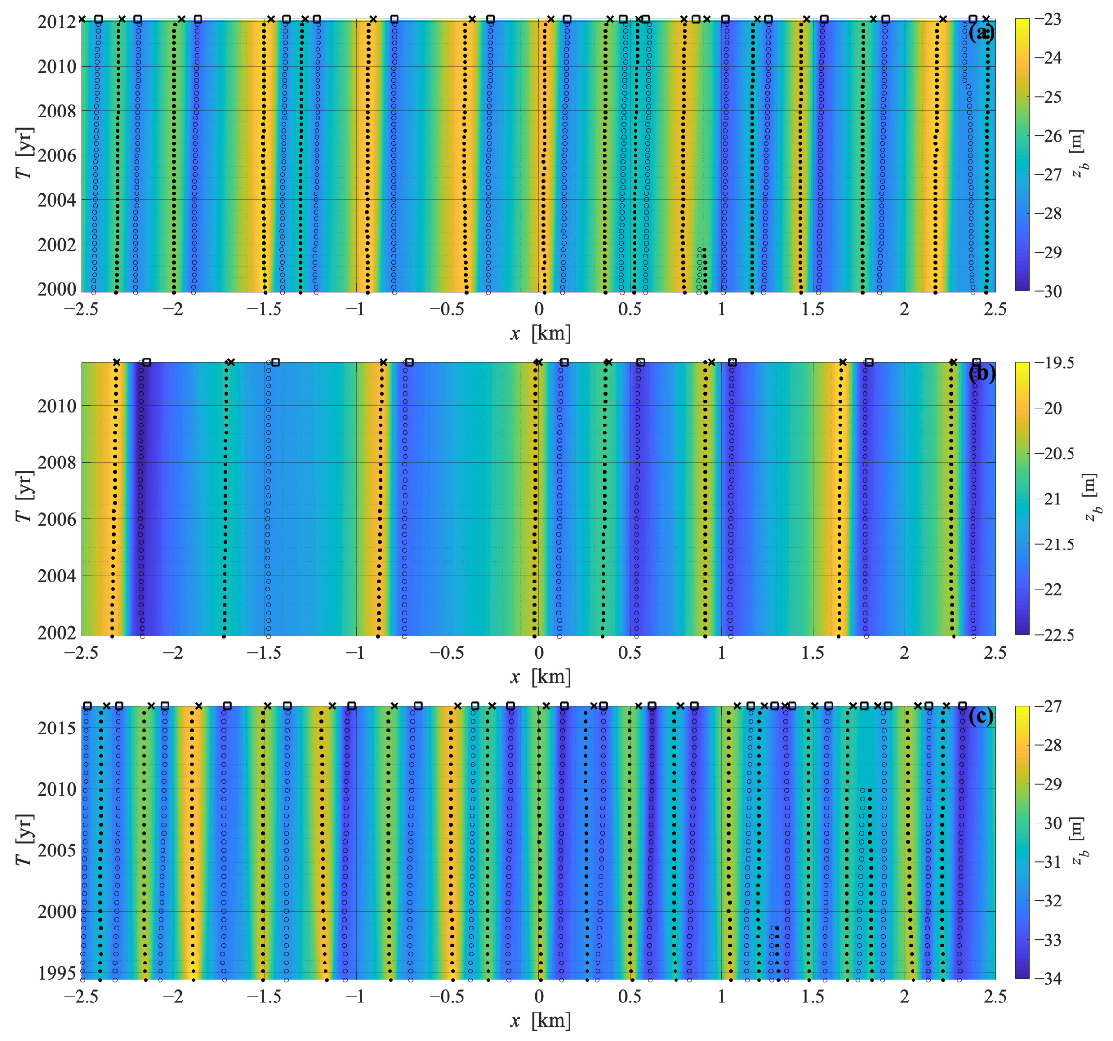
3.2. Validation
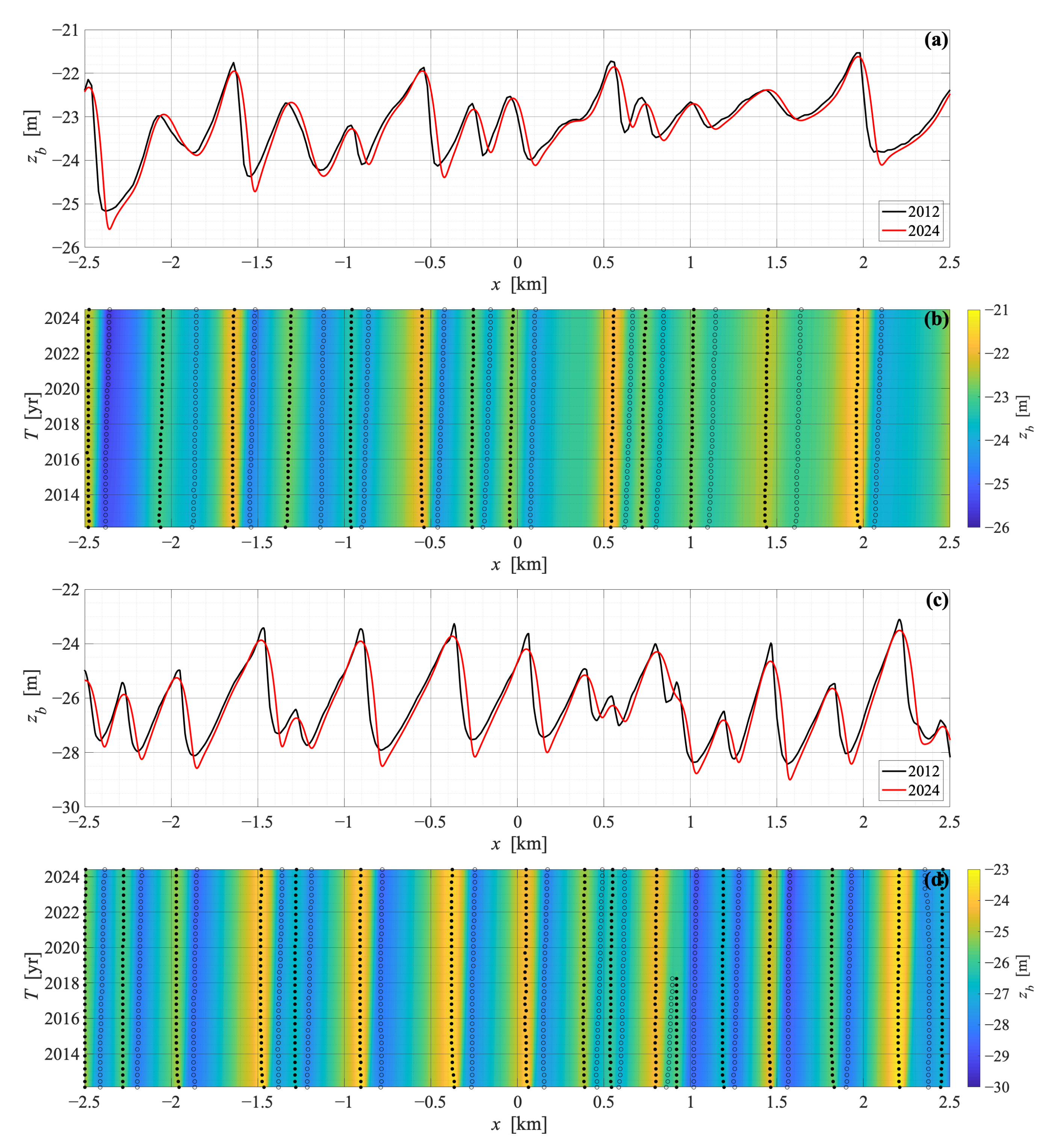
3.3. Forecast
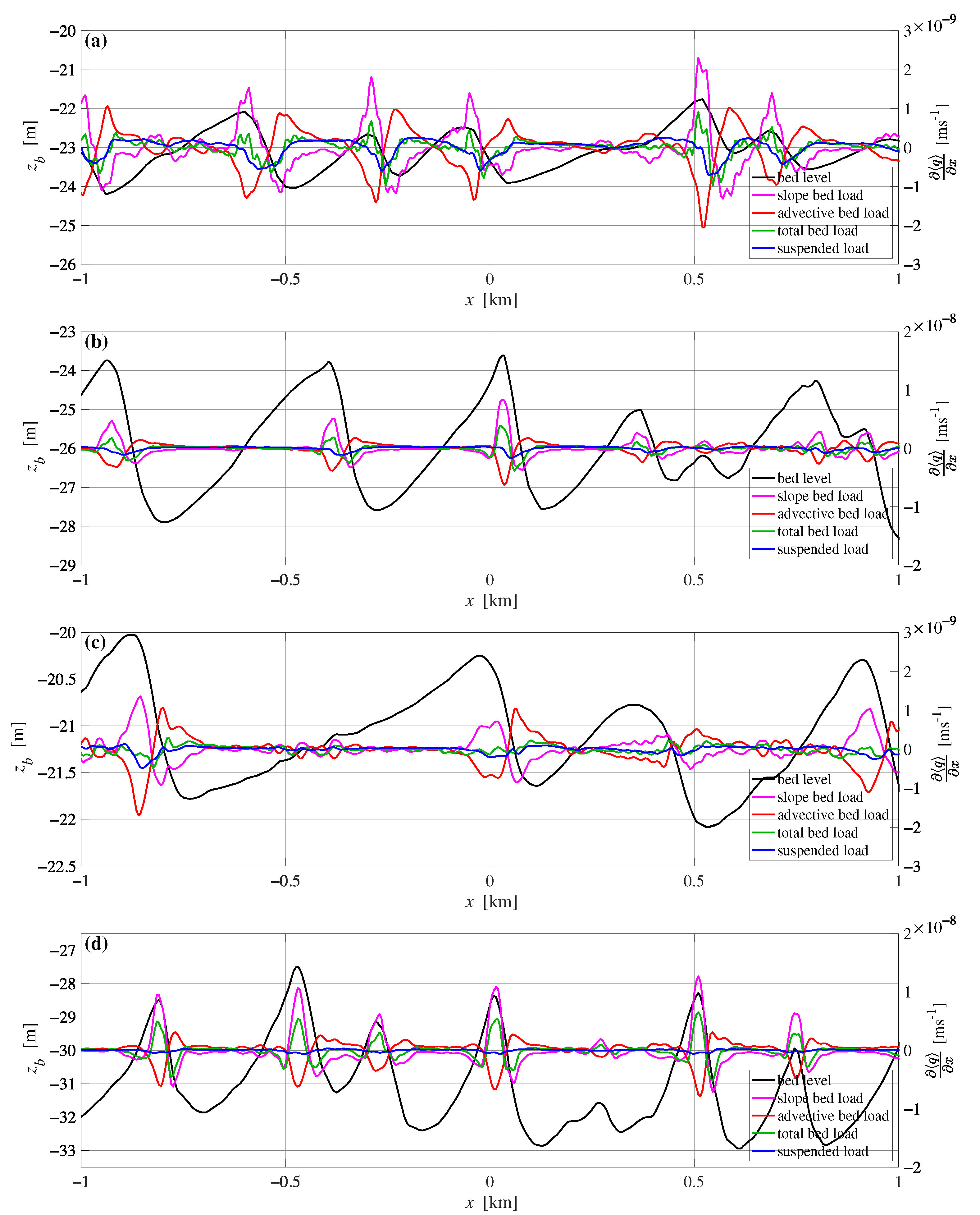
4. Discussion
5. Conclusions
Supplementary Materials
Author Contributions
Funding
Institutional Review Board Statement
Informed Consent Statement
Data Availability Statement
Acknowledgments
Conflicts of Interest
References
- McCave, I.N. Sand waves in the North Sea off the coast of Holland. Mar. Geol. 1971, 10, 199–225. [Google Scholar] [CrossRef]
- Lobo, F.; Hernández-Molina, F.; Somoza, L.; Rodero, J.; Maldonado, A.; Barnolas, A. Patterns of bottom current flow deduced from dune asymmetries over the Gulf of Cadiz shelf (southwest Spain). Mar. Geol. 2000, 164, 91–117. [Google Scholar] [CrossRef]
- Van Landeghem, K.J.; Uehara, K.; Wheeler, A.J.; Mitchell, N.C.; Scourse, J.D. Post-glacial sediment dynamics in the Irish Sea and sediment wave morphology: Data–model comparisons. Cont. Shelf Res. 2009, 29, 1723–1736. [Google Scholar] [CrossRef]
- Katoh, K.; Kume, H.; Kuroki, K.; Hasegawa, J. The Development of Sand Waves and the Maintenance of Navigation Channels in the Bisanseto Sea. Coast. Eng. 1998, 3490–3502. [Google Scholar] [CrossRef]
- Duffy, G.P.; Hughes-Clarke, J.E. Application of spatial cross correlation to detection of migration of submarine sand dunes. J. Geophys. Res. Earth Surf. 2005, 110. [Google Scholar] [CrossRef]
- Besio, G.; Blondeaux, P.; Brocchini, M.; Hulscher, S.J.; Idier, D.; Knaapen, M.A.; Németh, A.A.; Roos, P.C.; Vittori, G. The morphodynamics of tidal sand waves: A model overview. Coast. Eng. 2008, 55, 657–670. [Google Scholar] [CrossRef]
- Det Norske Veritas. Subsea Power Cables in Shallow Water Renewable Energy Applications, Report DNV-RP-J301; Det Norske Veritas: Høvik, Norway, 2014. [Google Scholar]
- Paulsen, B.T.; Roetert, T.; Raaijmakers, T.; Forzoni, A.; Hoekstra, R.; Van Steijn, P. Morphodynamics of Hollandse Kust (zuid) Wind Farm Zone, Report 1230851-000-HYE-0003; Deltares: Delft, The Netherlands, 2016. [Google Scholar]
- Raaijmakers, T.; Roetert, T.; Bruinsma, N.; Riezebos, H.J.; Van Dijk, T.; Forzoni, A.; Vergouwen, S.; Grasmeijer, B. Morphodynamics and Scour Mitigation for Hollandse Kust (noord) Wind Farm Zone, Report 11202796-000-HYE-0002; Deltares: Delft, The Netherlands, 2019. [Google Scholar]
- Hulscher, S.J.M.H. Tidal-induced large-scale regular form patterns in a three-dimensional shallow water model. J. Geophys. Res. 1996, 101, 20727–20744. [Google Scholar] [CrossRef]
- Besio, G.; Blondeaux, P.; Brocchini, M.; Vittori, G. On the modeling of sand wave migration. J. Geophys. Res. Oceans 2004, 109. [Google Scholar] [CrossRef]
- Leenders, S.; Damveld, J.; Schouten, J.; Hoekstra, R.; Roetert, T.; Borsje, B. Numerical modelling of the migration direction of tidal sand waves over sand banks. Coast. Eng. 2021, 163, 103790. [Google Scholar] [CrossRef]
- Dodd, N.; Blondeaux, P.; Calvete, D.; de Swart, H.E.; Falqués, A.; Hulscher, S.J.M.H.; Rózyński, G.; Vittori, G. Understanding Coastal Morphodynamics Using Stability Methods. J. Coastal Res. 2003, 19, 849–865. [Google Scholar]
- Fredsøe, J.; Deigaard, R. Mechanics of Coastal Sediment Transport; World Scientific: Singapore, 1992; Volume 3, pp. 265–279. [Google Scholar] [CrossRef]
- Knaapen, M.A.; Hulscher, S.J. Regeneration of sand waves after dredging. Coast. Eng. 2002, 46, 277–289. [Google Scholar] [CrossRef]
- Van Rijn, L.C. Principles of Sedimentation and Erosion Engineering in Rivers, Estuaries and Coastal Seas Including Mathematical Modelling Package (Toolkit on CD-ROM); Aqua Publications: Amsterdam, The Netherlands, 2005. [Google Scholar]
- Knaapen, M.A.F. Sandwave migration predictor based on shape information. J. Geophys. Res. Earth Surf. 2005, 110, 1–9. [Google Scholar] [CrossRef]
- Blondeaux, P.; Vittori, G. A model to predict the migration of sand waves in shallow tidal seas. Cont. Shelf Res. 2016, 112, 31–45. [Google Scholar] [CrossRef]
- Németh, A.A.; Hulscher, S.J.; Van Damme, R.M. Modelling offshore sand wave evolution. Cont. Shelf Res. 2007, 27, 713–728. [Google Scholar] [CrossRef]
- Van den Berg, J.; Sterlini, F.; Hulscher, S.J.; Van Damme, R. Non-linear process based modelling of offshore sand waves. Cont. Shelf Res. 2012, 37, 26–35. [Google Scholar] [CrossRef]
- Campmans, G.H.; Roos, P.C.; de Vriend, H.J.; Hulscher, S.J. The Influence of Storms on Sand Wave Evolution: A Nonlinear Idealized Modeling Approach. J. Geophys. Res. Earth Surf. 2018, 123, 2070–2086. [Google Scholar] [CrossRef]
- Van Gerwen, W.; Borsje, B.W.; Damveld, J.H.; Hulscher, S.J. Modelling the effect of suspended load transport and tidal asymmetry on the equilibrium tidal sand wave height. Coast. Eng. 2018, 136, 56–64. [Google Scholar] [CrossRef]
- Lesser, G.R.; Roelvink, J.A.; van Kester, J.A.; Stelling, G.S. Development and validation of a three-dimensional morphological model. Coast. Eng. 2004, 51, 883–915. [Google Scholar] [CrossRef]
- Komarova, N.L.; Newell, A.C. Nonlinear dynamics of sand banks and sand waves. J. Fluid Mech. 2000, 415, 285–321. [Google Scholar] [CrossRef]
- Hydrographic Service of the Royal Netherlands Navy. Hydrographic Surveys. 2017. Available online: http://opendap.deltares.nl/thredds/catalog/opendap/hydrografie/surveys/catalog.html (accessed on 17 November 2018).
- Dastgheib, A.; Roelvink, J.; Wang, Z. Long-term process-based morphological modeling of the Marsdiep Tidal Basin. Mar. Geol. 2008, 256, 90–100. [Google Scholar] [CrossRef]
- Zijl, F. Development of the next generation Dutch Continental Shelf Flood Forecasting Models, Memo, 1205989-003-ZKS-0002; Deltares: Delft, The Netherlands, 2013. [Google Scholar]
- Zijl, F.; Verlaan, M.; Gerritsen, H. Improved water-level forecasting for the Northwest European Shelf and North Sea through direct modelling of tide, surge and non-linear interaction. Ocean Dyn. 2013, 63, 823–847. [Google Scholar] [CrossRef]
- Van De Kreeke, J.; Robaczewska, K. Tide-induced residual transport of coarse sediment; Application To the Ems Estuary. Neth. J. Sea Res. 1993, 31, 209–220. [Google Scholar] [CrossRef]
- Fugro. Geophysical Site Investigation Survey/Hollandse Kust (Zuid) Wind Farm Development Zone/Wind Farm Site I to IV/Report GH176-R1-4; Fugro: Nootdorp, The Netherlands, 2016; Volume B. [Google Scholar]
- Fugro. Geophysical Site Investigation Survey/Hollandse Kust (noord) Wind Farm Survey 2017/Report GH216-R3; Fugro: Nootdorp, The Netherlands, 2018; Volume 3. [Google Scholar]
- Damen, J.M.; van Dijk, T.A.; Hulscher, S.J. Spatially Varying Environmental Properties Controlling Observed Sand Wave Morphology. J. Geophys. Res. Earth Surf. 2018, 123, 262–280. [Google Scholar] [CrossRef]
- Van Dijk, T.A.; Kleinhans, M.G. Processes controlling the dynamics of compound sand waves in the North Sea, Netherlands. J. Geophys. Res. Earth Surf. 2005, 110, 1–15. [Google Scholar] [CrossRef]
- Borsje, B.W.; Roos, P.C.; Kranenburg, W.M.; Hulscher, S.J. Modeling tidal sand wave formation in a numerical shallow water model: The role of turbulence formulation. Cont. Shelf Res. 2013, 60, 17–27. [Google Scholar] [CrossRef]
- Borsje, B.W.; Kranenburg, W.M.; Roos, P.C.; Matthieu, J.; Hulscher, S.J. The role of suspended load transport in the occurence of tidal sand waves. J. Geophys. Res. Earth Surf. 2014, 119, 701–716. [Google Scholar] [CrossRef]
- Deltares. Delft3D 3D-FLOW User Manual, Version: 3.15.34158; Deltares: Delft, The Netherlands, 2014. [Google Scholar]
- Engquist, B.; Majda, A. Absorbing boundary conditions for the numerical simulation of waves. Math. Comput. 1977, 31, 629–651. [Google Scholar] [CrossRef]
- Verboom, G.K.; Slob, A. Weakly-reflective boundary conditions for two-dimensional shallow water flow problems. Adv. Water Resour. 1984, 7, 192–197. [Google Scholar] [CrossRef]
- Van Rijn, L.C. Principles of Sediment Transport in Rivers, Estuaries and Coastal Seas; Aqua Publications: Amsterdam, The Netherlands, 1993. [Google Scholar] [CrossRef]
- Bagnold, R.A. An Approach to the Sediment Transport Problem From General Physics, in US Geological Survey Professional Paper 422-I; U.S. Government Printing Office: Washington, DC, USA, 1966; pp. 1–37. [CrossRef]
- Sleath, J.F. Sea Bed Mechanics; McCormick, M.E., Ed.; Wiley: Hoboken, NJ, USA, 1984. [Google Scholar]
- Maljers, D.; Gunnink, J. Interpolation of Measured Grain-Size Fractions. 2007. Available online: http://www.emodnet-seabedhabitats.eu/pdf/Imares_Interpolation%20of%20measured%20grain-size%20fractions.pdf (accessed on 17 May 2020).
- Sutherland, J.; Peet, A.; Soulsby, R. Evaluating the performance of morphological models. Coast. Eng. 2004, 51, 917–939. [Google Scholar] [CrossRef]
- Murphy, A.H.; Epstein, E.S. Skill scores and correlation coefficients in model verification. Mon. Weather Rev. 1989, 117, 572–582. [Google Scholar] [CrossRef]
- International Hydrographic Organization. IHO Standards for Hydrographic Surveys—IHO Publication No. 44; International Hydrographic Bureau: Monte-Carlo, Monaco, 2008; Volume 6. [Google Scholar]
- Garnier, R.; Calvete, D.; Falqués, A.; Caballeria, M. Generation and nonlinear evolution of shore-oblique/transverse sand bars. J. Fluid Mech. 2006, 567, 327–360. [Google Scholar] [CrossRef]
- Vis-Star, N.C.; De Swart, H.; Calvete, D. Patch behaviour and predictability properties of modelled finite-amplitude sand ridges on the inner shelf. Nonlin. Processes Geophys. 2008, 15, 943–955. [Google Scholar] [CrossRef]
- Dam, G.; Van der Wegen, M.; Labeur, R.; Roelvink, D. Modeling centuries of estuarine morphodynamics in the Western Scheldt estuary. Geophys. Res. Lett. 2016, 43, 3839–3847. [Google Scholar] [CrossRef]
- Blondeaux, P.; Vittori, G. Three-dimensional tidal sand waves. J. Fluid Mech. 2009, 618, 1–11. [Google Scholar] [CrossRef]
- Ranasinghe, R.; Swinkels, C.; Luijendijk, A.; Roelvink, D.; Bosboom, J.; Stive, M.; Walstra, D. Morphodynamic upscaling with the MORFAC approach: Dependencies and sensitivities. Coast. Eng. 2011, 58, 806–811. [Google Scholar] [CrossRef]
- Blondeaux, P.; Vittori, G. Formation of tidal sand waves: Effects of the spring - neap cycle. J. Geophys. Res. Oceans 2010, 115. [Google Scholar] [CrossRef]
- Reistad, M.; Breivik, Ø.; Haakenstad, H.; Aarnes, O.J.; Furevik, B.R.; Bidlot, J.R. A high-resolution hindcast of wind and waves for the North Sea, the Norwegian Sea, and the Barents Sea. J. Geophys. Res. Oceans 2011, 116. [Google Scholar] [CrossRef]
- Passchier, S.; Kleinhans, M. Observations of sand waves, megaripples, and hummocks in the Dutch coastal area and their relation to currents and combined flow conditions. J. Geophys. Res. Earth Surf. 2005, 110. [Google Scholar] [CrossRef]
- Van Oyen, T.; Blondeaux, P.; Van Den Eynde, D. Sediment sorting along tidal sand waves: A comparison between field observations and theoretical predictions. Cont. Shelf Res. 2013, 63, 23–33. [Google Scholar] [CrossRef]
- Damveld, J.H.; van der Reijden, K.J.; Cheng, C.; Koop, L.; Haaksma, L.R.; Walsh, C.A.; Soetaert, K.; Borsje, B.W.; Govers, L.L.; Roos, P.C.; et al. Video transects reveal that tidal sand waves affect the spatial distribution of benthic organisms and sand ripples. Geophys. Res. Lett. 2018, 45, 11837–11846. [Google Scholar] [CrossRef]
- Damveld, J.; Borsje, B.; Roos, P.; Hulscher, S. Horizontal and Vertical Sediment Sorting in Tidal Sand Waves: Modeling the Finite-Amplitude Stage. J. Geophys. Res. Earth Surf. 2020, 125. [Google Scholar] [CrossRef]
- Damveld, J.H.; Borsje, B.W.; Roos, P.C.; Hulscher, S.J. Biogeomorphology in the marine landscape: Modelling the feedbacks between patches of the polychaete worm Lanice conchilega and tidal sand waves. Earth Surf. Processes Landforms 2020, 45, 2572–2587. [Google Scholar] [CrossRef]


| Loc 1 | , | , | ||
|---|---|---|---|---|
| Amplitude | Phase | Amplitude | Phase | |
| M | 1.02 ms | 73 | 0.38 ms | 73 |
| M | 0.14 ms | 108 | 0.06 ms | 296 |
| M | 0.05 ms | 92 | 0.04 ms | 89 |
| M | 0.02 ms | −0.001 ms |
| Parameter | Symbol | Transect 1 | Transect 2 | Transect 3 | Transect 4 | Dimension |
|---|---|---|---|---|---|---|
| Domain length | L | 50 | 50 | 50 | 50 | km |
| Length of area of interest | ℓ | 5 | 5 | 5 | 5 | km |
| Undisturbed water depth | 23.6 | 26.3 | 21.3 | 30.7 | m | |
| Roughness length | 0.0944 | 0.0945 | 0.0945 | 0.0949 | m | |
| Median sand grain size | 0.275 | 0.305 | 0.305 | 0.390 | mm | |
| Bed slope parameter | 5.5 | 5.5 | 5.5 | 5.5 | - | |
| Sand transport scale factor | f | 0.45 | 0.45 | 0.45 | 0.45 | - |
| Hydrodynamic time step | 6 | 6 | 6 | 6 | s | |
| Horizontal grid spacing | 5 | 5 | 5 | 5 | m | |
| No of -layers | - | 40 | 40 | 40 | 40 | - |
| Morphological acceleration factor | MORFAC | 148 | 148 | 148 | 148 | - |
| Morphological simulation time | 12.3 | 12.3 | 9.7 | 22.4 | years |
| Runs | Description |
|---|---|
| H1–32 | Hindcast runs transect 1 with f varying between |
| 0.3 and 1 and varying between 3 and 6 | |
| V2–4 | Hindcast runs transects 2–4 with and |
| F1–2 | Forecast runs transects 1–2 with and |
| Transect 1 | ||
|---|---|---|
| Observations | Model | |
| 2.9 m yr | 1.1 m yr | |
| 1.3 m yr | 1.0 m yr | |
| 1.9 m yr | 2.9 m yr | |
| 0.9 m yr | 0.7 m yr | |
| RMSE | 0.13 m | |
| RMSE | 27.0 m | |
| RMSE | 0.21 m | |
| RMSE | 16.8 m | |
| RMSE | 0.17 m | |
| 0.74 | ||
| 0.01 | ||
| 0.01 | ||
| 0.01 | ||
| BSS | 0.74 | |
| Transect 2 | Transect 3 | Transect 4 | ||||
|---|---|---|---|---|---|---|
| Observations | Model | Observations | Model | Observations | Model | |
| 2.2 m yr | 0.4 m yr | 2.8 m yr | 1.0 m yr | 1.3 m yr | −0.4 m yr | |
| 1.2 m yr | 0.6 m yr | 1.2 m yr | 1.2 m yr | 0.2 m yr | 0.5 m yr | |
| 1.1 m yr | 1.3 m yr | 2.3 m yr | 0.3 m yr | 1.0 m yr | 0.6 m yr | |
| 1.1 m yr | 1.4 m yr | 0.9 m yr | 0.5 m yr | 0.5 m yr | 0.5 m yr | |
| RMSE | 0.44 m | 0.12 m | 1.04 m | |||
| RMSE | 28.7 m | 19.7 m | 38.7 m | |||
| RMSE | 0.42 m | 0.22 m | 0.55 m | |||
| RMSE | 14.5 m | 22.5 m | 14.3 m | |||
| RMSE | 0.35 m | 0.13 m | 0.72 m | |||
| 0.57 | 0.26 | 0.27 | ||||
| 0.03 | 0.02 | 0.01 | ||||
| 0.01 | 0.02 | 0.01 | ||||
| 0.01 | 0.02 | 0.01 | ||||
| BSS | 0.54 | 0.24 | 0.26 | |||
| Transect 1 | Transect 2 | Transect 3 | Transect 4 | |
|---|---|---|---|---|
| 0.027 yr | 0.031 yr | 0.0226 yr | 0.054 yr | |
| −0.027 yr | −0.033 yr | −0.017 yr | −0.076 yr | |
| 0.000 yr | −0.002 yr | 0.006 yr | −0.022 yr | |
| 0.002 yr | 0.004 yr | 0.003 yr | 0.006 yr | |
| 0.461 m yr | 0.387 m yr | −0.198 m yr | −0.135 m yr | |
| 0.598 m yr | 0.755 m yr | 0.447 m yr | 0.844 m yr | |
| 1.059 m yr | 1.142 m yr | 0.249 m yr | 0.710 m yr | |
| 1.070 m yr | 0.779 m yr | 0.485 m yr | 0.067 m yr |
Publisher’s Note: MDPI stays neutral with regard to jurisdictional claims in published maps and institutional affiliations. |
© 2021 by the authors. Licensee MDPI, Basel, Switzerland. This article is an open access article distributed under the terms and conditions of the Creative Commons Attribution (CC BY) license (https://creativecommons.org/licenses/by/4.0/).
Share and Cite
Krabbendam, J.; Nnafie, A.; de Swart, H.; Borsje, B.; Perk, L. Modelling the Past and Future Evolution of Tidal Sand Waves. J. Mar. Sci. Eng. 2021, 9, 1071. https://doi.org/10.3390/jmse9101071
Krabbendam J, Nnafie A, de Swart H, Borsje B, Perk L. Modelling the Past and Future Evolution of Tidal Sand Waves. Journal of Marine Science and Engineering. 2021; 9(10):1071. https://doi.org/10.3390/jmse9101071
Chicago/Turabian StyleKrabbendam, Janneke, Abdel Nnafie, Huib de Swart, Bas Borsje, and Luitze Perk. 2021. "Modelling the Past and Future Evolution of Tidal Sand Waves" Journal of Marine Science and Engineering 9, no. 10: 1071. https://doi.org/10.3390/jmse9101071
APA StyleKrabbendam, J., Nnafie, A., de Swart, H., Borsje, B., & Perk, L. (2021). Modelling the Past and Future Evolution of Tidal Sand Waves. Journal of Marine Science and Engineering, 9(10), 1071. https://doi.org/10.3390/jmse9101071