Evolution Characteristics of Suction-Side-Perpendicular Cavitating Vortex in Axial Flow Pump under Low Flow Condition

Abstract

In order to study the evolution characteristics of suction-side-perpendicular cavitating vortex in an axial-flow pump under low flow conditions, model tests, high-speed imaging, and an SST-CC turbulence model were used to simulate the external characteristics and cavitation morphology of the pump. The evolution law of suction-side-perpendicular cavitating vortex (SSPCV) was revealed by turbulent kinetic energy, liutex vortex identification, and vorticity transport equation. The results show that the evolution of suction-side-perpendicular cavitating vortex at low cavitation number can be divided into three stages: generation, development, and breaking stage. In the generation stage, the turbulent kinetic energy, velocity gradient and vortex kinetic energy continue to increase, reaching the maximum at the early stage of development. Afterwards, due to the viscosity of the water, the vortex slowly dissipates and enters the stage of development. Finally, it is affected by the next blade and enters the breaking stage, which accelerates the dissipation of the vortex. The vortex stretching term and vortex expansion term are the main contributors to the vorticity. During the development of the vortex, the vorticity is mainly caused by the deformation of the fluid micelle. The breaking stage mainly affects the stretching term, and the Coriolis force term cannot be ignored in the rotating coordinates.

1. Introduction

Cavitation is a very common phenomenon in hydraulic machinery. Periodic growth and rupture of cavitation will lead to vibration, noise, and a sudden drop of hydraulic performance [1]. Cavitation involves a wide range of fields and has been studied by scholars all over the world. Some scholars have used water tunnels to study the mechanism of cavitation [2,3,4], using high-speed photography and PIV instruments and numerical simulation techniques to obtain the formation, evolution, and destruction mechanism of hydrofoil cavitation. Ebrahim Kadivar et al. studied CAV2003 hydrofoil passive flow control under different cavitation conditions using cylindrical miniature vortex generators, obtained cavitation structure and average velocity distribution by using high-speed photography and PIV technology, and analyzed pressure pulsation at the tail of airfoil [5]. Cavitation research has also been applied to various hydraulic machinery. In the study of cavitation of the turbo pump inducer [6,7,8], the cavitation study of the different parameters and grooving measures of the inducer is carried out. Bensow et al. used LES method to study the cavitation of propeller [9] and Andreas Peters used RANS and VOF methods to predict the cavitation erosion capacity of propeller [10]. Pardeep Kumar et al. Summarized and reviewed cavitation types, vibration and noise, cavitation prevention, and control in hydraulic turbines [11]. Other forms of pump cavitation and vortex interaction are also studied, and vorticity transport equations are introduced to analyze vorticity and each item in the pump, to study the action mechanism of cavitation and vortex, and to explore the effect of different terms on vorticity [12,13,14].

Studies on cavitation in axial-flow pumps are mainly focused on the tip region. For example, Desheng Zhang et al. conducted a large number of studies on the morphology, development, and evolution of cavitation and leakage vortex in the tip region through numerical simulation combined with high-speed photography [15,16,17]. Suction-side-perpendicular cavitating vortex is a complex phenomenon of cavitation and vortex in the tip area; Shen Xi [18] and Desheng Zhang [19] explained the development process of SSPCV through high-speed photography and numerical simulation. The results showed that, once the SSPCV is formed, it will block the flow channel and reduce the flow in the tip area, which has a great impact on the whole leaf top area.

There are few studies on the evolution characteristics of suction-side-perpendicular cavitating vortex in the existing literature. This paper takes the axial-flow pump as the research object to study the evolution characteristics of SSPCV, so as to obtain the development law of SSPCV, deepen the understanding of axial-flow pump cavitation, and provide reference for improving the cavitation performance of pump. The article verifies the correctness of the numerical simulation through external characteristics and high-speed photography, and analyzes the evolution process of the SSPCV, the turbulent kinetic energy and turbulent viscosity. The liutex method was used to identify vortexes in axial-flow pumps. The evolution mechanism of vortices was explored through velocity gradient and vortex kinetic energy, and the vorticity transport equation was introduced to compare the contributions of each component to vorticity. Finally, these methods are compared.

2. Test Model Device and Numerical Simulation Method

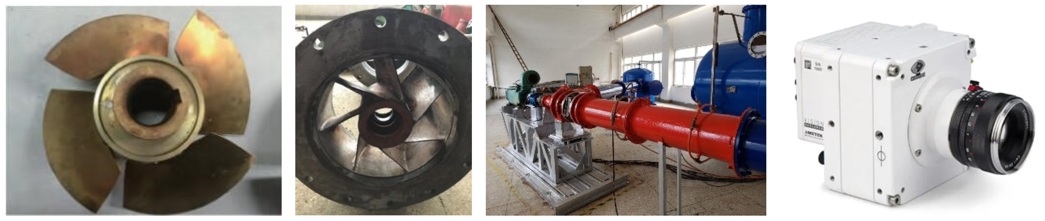
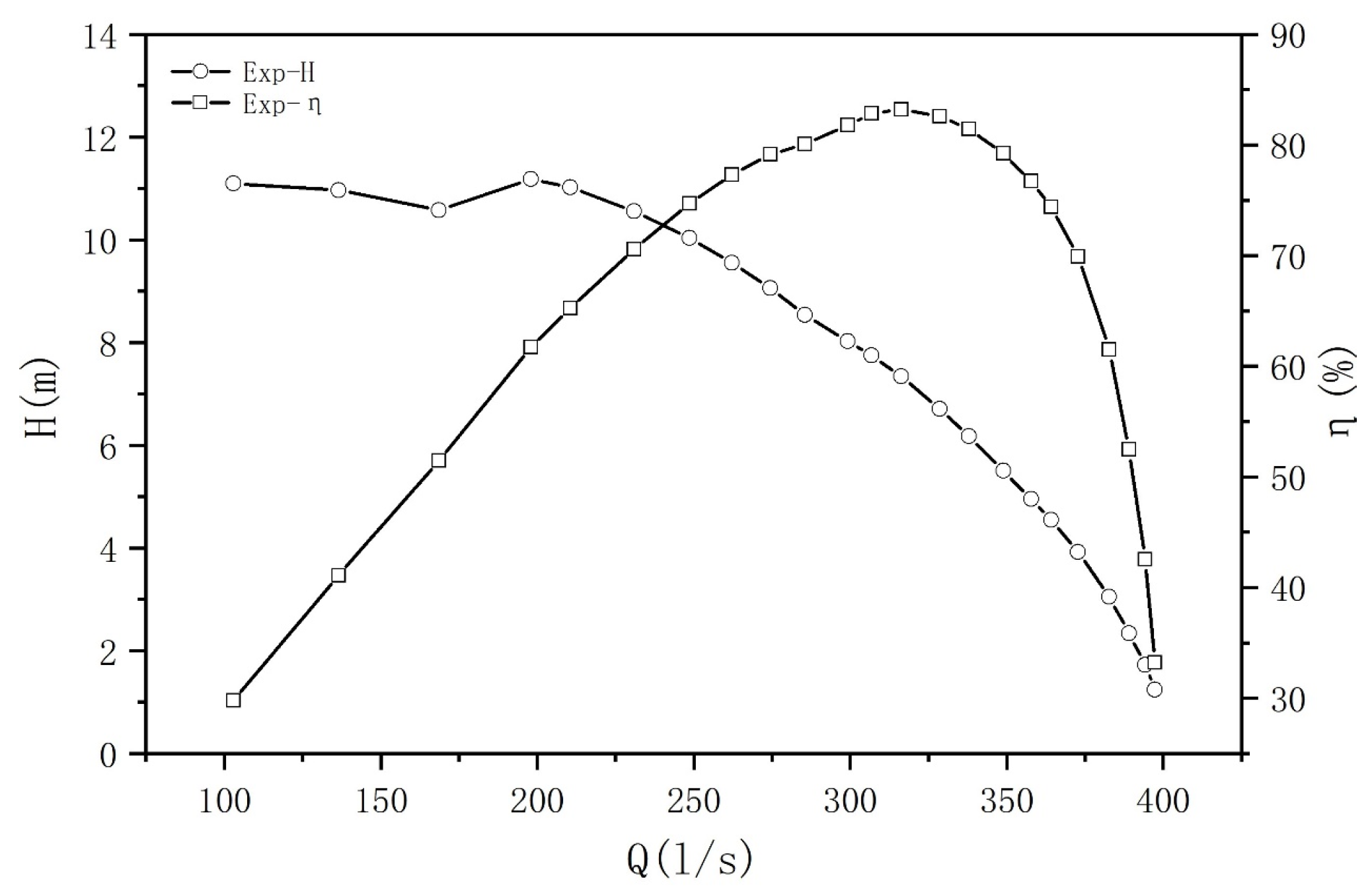
2.1. Model Test

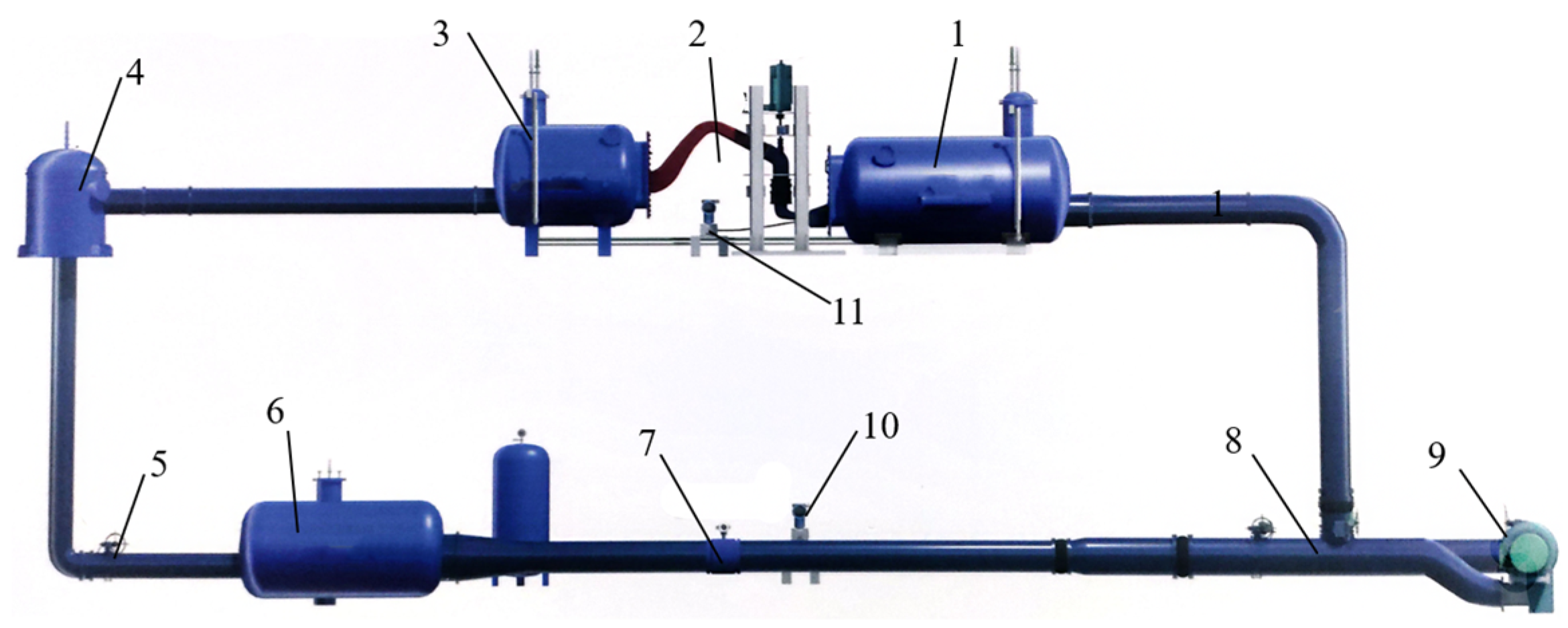
2.1.1. Experimental Equipment and Instruments

The test was carried out on the high-precision hydraulic machinery test bench of Yangzhou University. The structure and composition of the test bench are shown in Figure 1. A TJ-ZL-24G impeller and matching guide vane are used for the pump section experiment. The impeller had a diameter of 300 mm and a rated speed of 1450 r/min. The pump section was composed of inlet pipe, impeller, guide vane, and outlet pipe. The experimental model and high-speed camera are shown in the Figure 2. The test was carried out in accordance with “Hydraulic Performance Test Specification for Centrifugal Pumps, Mixed flow Pumps and Axial Flow Pumps (Precision Level)” (GB/T18149–2017) and “Acceptance Test Specification for Pump Model and Device Model” (SL140–2006).

Veo710l high-speed camera was used to take cavitation photos of pump section through the observation window of impeller chamber of pump section. The high-speed camera used 1280 × 800 CMOS sensor. The full-frame shooting rate was 7400 frames/s, and the highest rate was 1,000,000 frames/s, with advantages of high sensitivity and high resolution. We set up two spotlights for lighting during shooting to improve the imaging effect. The results were processed by the adaptive PCC software.

2.1.2. Uncertainty Analysis of Efficiency Test

• Uncertainty analysis of the test bench system

The primary sensor, differential pressure transmitter, and torque speed sensor used in the test of flow, head and torque, and speed, etc. have been verified by the measurement and calibration department recognized by the state. The system uncertainty of the performance and efficiency test of the pump on the test bed is the square and root of the uncertainty of each single system, namely:

$${\left(E_{\eta }\right)}_s=\pm \sqrt{E_Q^2+E_H^2+E_M^2+E_N^2}=\pm 0.274\%$$

(1)

where, $E_Q$ is the system uncertainty of flow measurement, and the full range of calibration result is ±0.2%; $E_H$ is the systematic uncertainty of static head measurement, and the calibration result of the full range is ±0.10%; $E_H$ is the systematic error of the head measurement of the device; $E_M$ is the system uncertainty of torque measurement, and the uncertainty of torque speed sensor is ±0.15%; and $E_N$ is the system uncertainty of speed measurement. When the sampling period of the measurement system is 2 s and the speed is not less than 1000 r/min, the uncertainty is ±0.05%.

2.

Random uncertainty of efficiency test

Under the condition of a stable design head, the uncertainty estimation of performance test is carried out according to the dispersion degree of efficiency measurement, and the calculation formula is as follows:

$${(E_{\eta })}_r=\pm \frac{t_{0.95(N-1)}\times S_{\overline{\eta }}}{\overline{\eta }}\times 100\%$$

(2)

where $S_{\overline{\eta }}$ means standard deviation of average efficiency value:

$$S_{\overline{\eta }}=\sqrt{{\displaystyle \sum \frac{{({\eta }_i-\overline{\eta })}^2}{(N-1)}}}$$

(3)

where $N$ is the number of measurements; ${\eta }_i$ is the ith efficiency measurement; $\overline{\eta }$ is average efficiency; and $t_{0.95 \left(N-1\right)}$ is the t-distribution value corresponding to 0.95 confidence rate and (N − 1) degrees of freedom, t = 2.26.

According to the actual measurement results: $\overline{\eta }=75.19\%$, $S_{\overline{\eta }}=0.036\%$

$$(E_{\eta }{)}_r=\pm 2.26\times 0.036\%/75.19\%=\pm 0.11\%$$

3.

Total uncertainty of efficiency test

$$E_{\eta }=\pm \sqrt{{\left(E_{\eta }\right)}_s^2+{\left(E_{\eta }\right)}_r^2}=\pm \sqrt{{(0.274\%)}^2+{(0.11\%)}^2}=\pm 0.296\%$$

(4)

It is higher than the requirement of the total uncertainty in the Acceptance Test Code for Pump Model and Device Model (SL140-2006).

2.2. Numerical Simulation

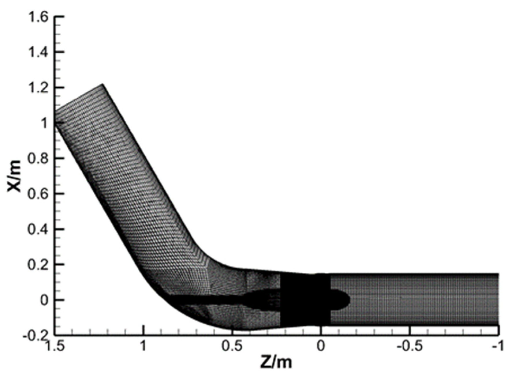
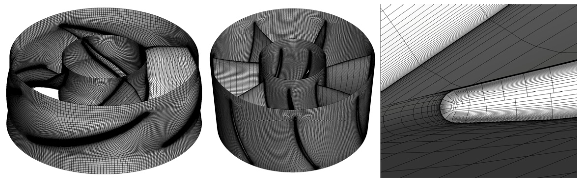
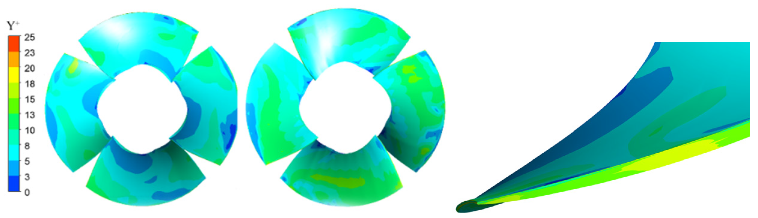
2.2.1. Grid Generation

The calculation model is shown in Figure 3. The grid of the impeller guide vane and the tip clearance is shown in Figure 4. The grid of inlet and outlet pipes is divided into structured grids with icem CFD software, and turbogrid software divides the grid of the impeller and guide vane. As the main research object is the impeller, the mesh of the impeller is encrypted. The Y+ of the main part of the pump section and the tip clearance is shown in Figure 5.

2.2.2. Governing Equation

Taking the time–mean N–S equation as the basic governing equation, an SST–CC (curvature correction) model was adopted. Based on SST k–ω model, curvature correction was carried out in this model. Through the correction coefficient $f_r$, the turbulence generation term $P_k$ was more sensitive to streamline curvature and rotational motion, so that the calculation results were more accurate. The simulation of the blade tip region is closer to the experiment. The correction coefficient $f_r$ is

$$f_r=\max \left[\min \left(f_{rot},1.25\right),0\right]$$

(5)

$$f_{rot }=\left(1+c_{r1}\right)f^{*}\left[1-c_{r3}\arctan \left(c_{r2}\tilde{r}\right)\right]-c_{r1}$$

(6)

$$f^{*}=\frac{2r^{*}}{1+r^{*}}$$

(7)

In the formula, $f_{rot}$ is the correction function considering the influence of rotation and curvature, $c_{r1}$, $c_{r2}$, and $c_{r3}$ are empirical constants, $f^{*}$ is rotation correction factor, and $r^{*}$ and $\tilde{r}$ are the functions of rotation speed of the system.

The revised turbulence model is

$$\frac{\partial ({\rho }_{m}k)}{\partial t}+\frac{\partial \left({\rho }_m{u}_{j}k\right)}{\partial x_j}=\frac{\partial }{\partial x_j}\left[\left({\mu }_m+\frac{{\mu }_t}{{\sigma }_k}\right)\frac{\partial k}{\partial x_j}\right]+f_r{P}_k-{\beta }^{*}{\rho }_m\omega k$$

(8)

$$\frac{\partial ({\rho }_m\omega )}{\partial t}+\frac{\partial \left({\rho }_m{u}_j\omega \right)}{\partial x_j}=\frac{\partial }{\partial x_j}\left[\left({\mu }_m+\frac{{\mu }_t}{{\sigma }_{\omega }}\right)\frac{\partial \omega }{\partial x_j}\right]+f_r\frac{\alpha \omega }{k}{P}_k-D_{\omega }+C{d}_{\omega }$$

(9)

$$\begin{array}{l}{\mu }_t=\frac{{\rho }_m{\alpha }_{1}k}{\max \left({\alpha }_1\omega ,S{F}_2\right)}\\ D_{\omega }=\beta {\rho }_m{\omega }^2,C=2{\rho }_m\left(1-F_1\right)\\ d_{\omega }=\frac{1}{\omega {\sigma }_{\omega 2}}\frac{\partial k}{\partial x_j}\frac{\partial \omega }{\partial x_j}\end{array}\}$$

(10)

where $k$ is turbulent kinetic energy; $\omega$ is turbulence frequency; $P_k$ is the production rate of turbulence; ${\rho }_m$ is the mixed density, kg/m³; $u_j$ is velocity component in j direction; ${\mu }_t$ is the turbulence viscosity and $\mu$ is the dynamic viscosity, Pa·s $F_1$ and $F_2$ are mixed functions; ${\beta }^{*}$, $\beta$, $\alpha$, ${\alpha }_1$, ${\alpha }_k$, ${\sigma }_{\omega }$, and ${\sigma }_{\omega 2}$ are all empirical coefficients; $S$ is the invariant of strain rate; $D_{\omega }$ is the dissipation term in $\mathsf{\omega }$-equation; and $C{d}_{\omega }$ is the cross-diffusion term in the SST model.

The cavitation model is Zwart model built in ANSYS CFX. For the simplified Rayleigh–Plesset equation, its expression is

$$m^{-}=-F_e\frac{3r_{nuc}\left(1-{\alpha }_v\right){\rho }_v}{R_B}\sqrt{\frac{2}{3}\frac{\left|p_v-p\right|}{{\rho }_l}},p<p_v$$

(11)

$$m^{+}=F_c\frac{3a_v{\rho }_v}{R_B}\sqrt{\frac{2}{3}\frac{\left|p_v-p\right|}{{\rho }_l}},p>p_v$$

(12)

where $m^{+}$ and $m^{-}$ are mass transfer source terms connected to the growth and collapse of the vapor bubbles, respectively; $F_e$ is evaporation coefficient, take 50; $F_c$ is coefficient of condensation, take 0.01; $r_{nuc}$ is nucleation site volume fraction, 5 × 10⁻⁴; $R_B$ is cavity radius, 1 × 10⁻⁶ m; ${\alpha }_v$ is vapor volume fraction; $p_v$ is saturation vapor pressure, 3574 Pa; ${\rho }_v$ is vapor density, 0.02308 kg/m³; and ${\rho }_l$ is liquid density, 997 kg/m³.

2.2.3. Boundary Conditions

The impeller rotating speed is set as 1450 r/min, the interface of dynamic and static is stage, the inlet is the total pressure inlet, the outlet is the mass flow outlet, and the inlet is set as 230 kg/s ($Q$ = 0.7$Q_d$, $Q_d$: design flow). The analysis type is set to steady, and the steady state solution is obtained by changing the inlet pressure.

The analysis type is set as transient, the interface of dynamic and static is set as transient rotor stator; the total time of 8 cycles is calculated as 0.3310344 s, and every 3° is a time step. Each cycle calculated 120 steps, each step iteration 15 times; each step time is 0.0003448275 s. The steady-state calculation results are taken as the initial conditions of the unsteady calculation. The last four cycles are used to analyze the results.

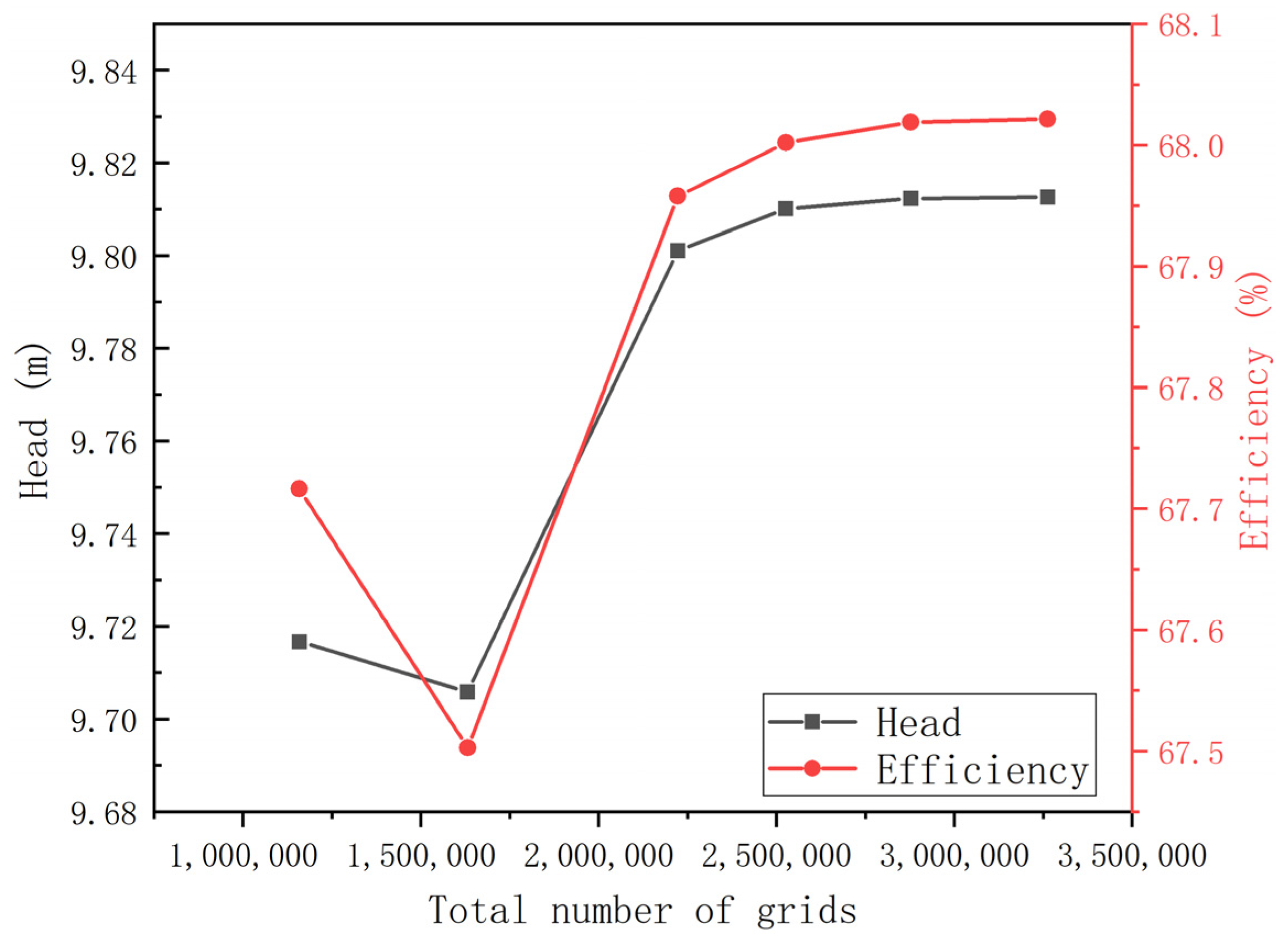
2.2.4. Grid-Independent Verification

The main area of simulation research is the impeller, and the grid of the impeller has a crucial impact on the whole simulation. Therefore, the grid independence is verified by changing the number of grids of the impeller. The inlet pipe grid is 480,000, the guide vane grid is 680,000, and the outlet pipe grid is 630,000. At the flow rate of 230 l/s, six groups of grids were selected for grid-independent analysis of impeller area. Head and efficiency under different grid numbers were obtained through steady-state calculation, as shown in Figure 6.

When the number of the impeller mesh exceeds 2.2 million, the head and efficiency tend to be stable. In order to coordinate the calculation efficiency and the calculation accuracy, the final selection of the grids number 2,526,040 schemes. The total number of grids in the computing domain is 4.32 million.

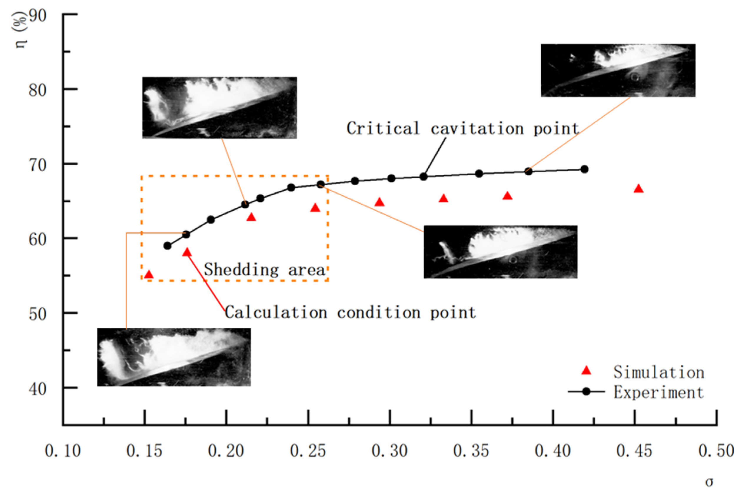
2.2.5. Comparison between Numerical Simulation and Experiment

The performance curve of TJ-ZL-24G pump is shown in Figure 7, with a design flow rate of 320 l/s, a design head of 7.34 m, and a maximum efficiency of 83.7%.

SSPCV are easier to observe under the condition of small flow, so the selected flow should be as small as possible in order to study the SSPCV and obtain their morphological changes. However, when the pump is running near the saddle area, as the rotating stall will generate blade passage vortex at the tail of the blade, and the vibration and noise are relatively large when running in the saddle area, there are many influencing factors. In order to exclude the influence of these factors, the flow rate should be at least more than 200 l/s, and the flow rate of 230 l/s is selected for analysis under comprehensive consideration.

Define the cavitation number:

$$\sigma =\frac{2\left(P_{in}-P_v\right)}{{\rho }_l{u}_{tip}^2}$$

(13)

here $P_{in}$ is the inlet pressure, Pa; and $u_{tip}$ is the speed at the rim, m/s.

Figure 8 shows the comparison of η–σ between numerical simulation and experiment at $Q$ = 0.7$Q_d$. Cavitation easily occurs at small flow rate, and efficiency decreases continuously with the decrease in inlet pressure. When the cavitation number is 0.32, the efficiency decreases by 1%, which is the critical cavitation point of the flow rate. When the cavitation number is 0.28, obvious loss begins to occur. When the cavitation number is about 0.18, it has entered the deep cavitation state. The maximum error between numerical simulation and experimental efficiency is 2.7%, and the relative error is 3%. The predicted cavitation trend is the same as the test trend.

Figure 8 also shows the cavitation morphology of blade tip area when the cavitation number is 0.38, 0.255, 0.22, and 0.18. When the cavitation number is 0.38, the shedding has not been formed. When the cavitation number is 0.255, obvious shedding has occurred, and the SSPCV is a small vortex line. When the cavitation number is further reduced to 0.22, shedding is already very obvious. When the cavitation number is 0.18, the degree of cavitation is more serious. Compared with when the cavitation number is 0.22, the SSPCV is more stable and develops for a longer time, which is convenient for studying its development law. Therefore, this condition is selected for research and analysis.

3. Results and Analysis

3.1. Cavitation Analysis

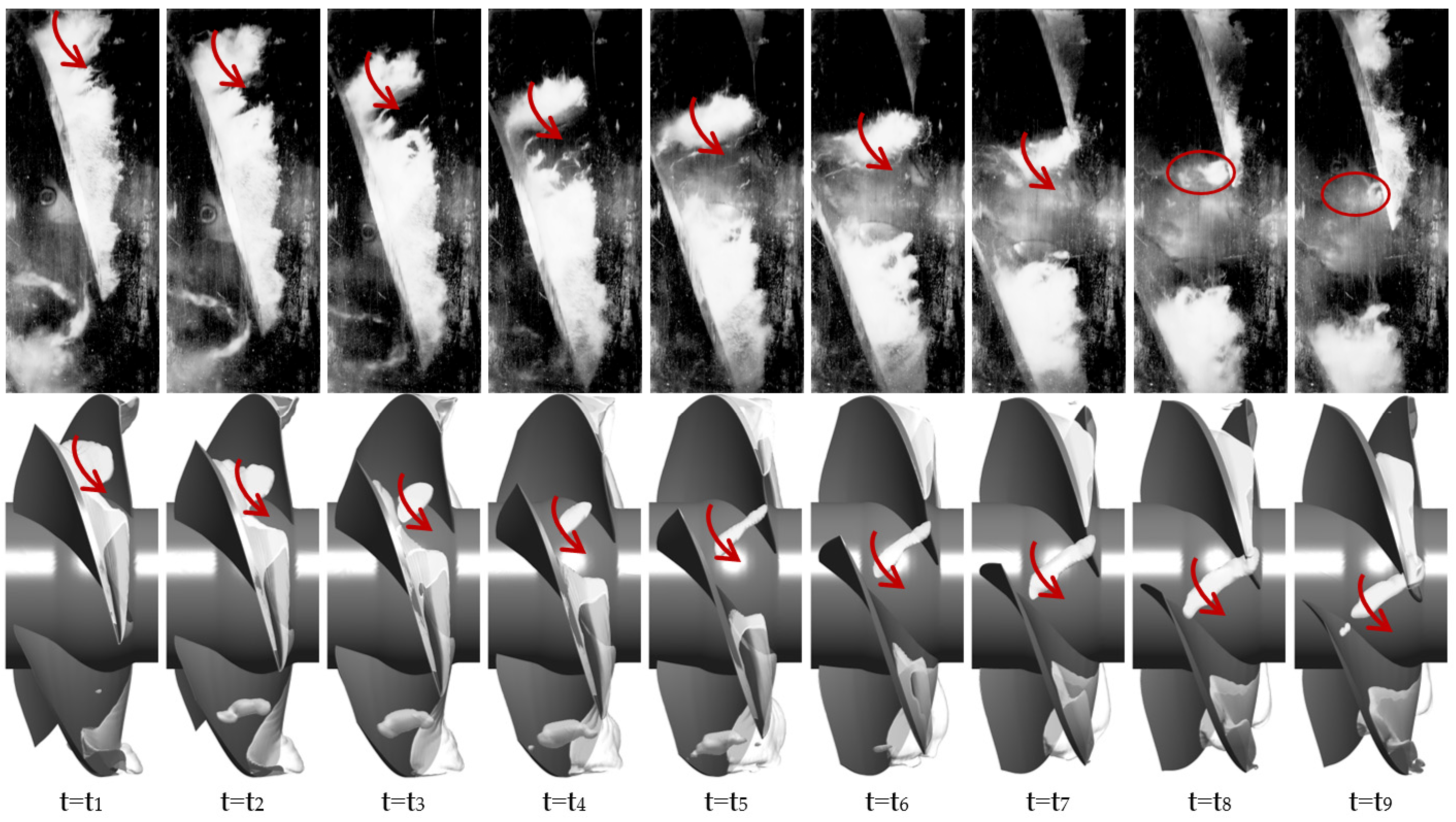
3.1.1. Cavitation Morphology Evolution Law

Figure 9 shows the comparison between numerical simulation and model test of cavitation shedding evolution of a blade in a cycle when the cavitation number is 0.18. The time interval is Δt = 0.0010344825 s, and the time of a shedding cycle is approximately 0.00827 s. The top of Figure 8 shows high-speed photography of cavitation. Under the working condition of deep cavitation, the cavitation length has reached 0.8 times of the blade length. Affected by the shedding of the last blade, the triangular area of the clearance cavitation head has a serrate structure, showing strong unsteady characteristics. At t = t₁, the cloud cavitation of the tip blade tail begins to separate, and the SSPCV is formed under the action of the tip clearance vortex. The rotation direction of the SSPCV is the same as the impeller. With the development of SSPCV from t = t₂ to t = t₆, the range of shedding cavitation becomes smaller and elongated. At t = t₇, cavitation develops to the head of the next blade, affecting the pressure distribution of the blade head. Then, the cavitation vortex is cut off by the blade. After the cut, the cavitation vortex does not disappear immediately and continues to dissipate backward, affecting the distribution of the pressure surface of the next blade and the distribution of the tip cavitation triangle region. The SSPCV not only blocks the flow passage and reduces the flow rate, but also changes the surface pressure of the blade and reduces the work capacity of the blade.

The bottom of Figure 9 shows the isosurface of the vapor volume fraction which α_v = 0.1. The evolution process of the SSPCV can be well predicted through the numerical simulation, which is basically consistent with the experiment and verifies the accuracy of the numerical simulation.

3.1.2. The Change of Turbulent Kinetic Energy and Eddy Viscosity of Cavitation Shedding

Figure 10 shows the variation of cavitation volume fraction, turbulent kinetic energy, and eddy viscosity with time at span = 0.9. Shedding cavitation is essentially the cloud cavitation produced by the hydrofoil in the tip area. Compare the position of the cavitation and analyze the changes of its turbulent kinetic energy and turbulent viscosity. From t = t₁ to t = t₄, the shedding gradually develops and forms. The turbulent kinetic energy core is at the position of 0.8 times the chord length and reaches its peak at t = t₄, when the cloud cavitation is shed and formed, and the sheet cavitation begins to shrink. From t = t₅ to t = t₉, the turbulent kinetic energy develops backward and gradually decreases as the falling cavitation develops backward. The turbulent kinetic energy in the blade passage keeps spreading, but it always keeps the maximum range near the tail of the hydrofoil. After the hydrofoil cloud cavitation falls off, the sheet cavitation length shrinks to 0.5 times the chord length. The turbulent kinetic energy also adheres to the position of 0.5 times the chord length, and the magnitude increases with the increase in sheet cavitation. In the process of cloud cavitation shedding, turbulent kinetic energy mainly shows in the middle and rear of the hydrofoil, and changes periodically, and reaches the peak at the moment of sheet cavitation retraction. Eddy viscosity shows the dissipation of vortex, which is mainly concentrated in the head of cavitation shedding. Eddy viscosity increases continuously, reaching 1.5 pa·s at t = t₆, and then decreases continuously. Eddy viscosity is larger at the upper part of SSPCV, indicating that the energy dissipation of vortex head is large.

3.2. Suction-Side-Perpendicular Cavitating Vortex

3.2.1. Identification of Vortices

Liutex is a new vortex identification method which can eliminate the shear pollution on the wall [20]. The motion decomposition of the rigid rotating part [21] is accurately captured from the fluid movement. First, the direction r of liutex is determined by $⟨\omega ,v_r⟩ > 0$. Then, Q rotation is used to rotate the initial x, y, z coordinate system to x_Q, y_Q, z_Q so that the rotated z_Q is the same as the rotation axis r. After rotation, the velocity gradient tensor $\nabla V_Q$ becomes:

$$\nabla V_Q=Q\nabla V{Q}^T=\left[\begin{array}{ccc}\frac{\partial u_Q}{\partial x_Q}& \frac{\partial u_Q}{\partial y_Q}& 0\\ \frac{\partial v_Q}{\partial x_Q}& \frac{\partial v_Q}{\partial y_Q}& 0\\ \frac{\partial w_Q}{\partial x_Q}& \frac{\partial w_Q}{\partial y_Q}& \frac{\partial w_Q}{\partial z_Q}\end{array}\right]$$

(14)

where $Q$ is the coordinate rotation matrix, and $\left(u_Q,v_Q,w_Q\right)$ is the velocity component in the $x_Q$, $y_Q$, $z_Q$ coordinate system after rotation.

Rotate the second P around $z_Q$, let the rotation Angle be $\theta$, then:

$$P=\left[\begin{array}{ccc}\cos \theta & \sin \theta & 0\\ -\sin \theta & \cos \theta & 0\\ 0& 0& 1\end{array}\right]$$

(15)

Then, the velocity gradient tensor after rotation of $P$ becomes:

$$\nabla V_{\theta }=P\nabla V_Q{P}^T$$

(16)

Then, the rotation strength is defined as 2 times of the minimum value of $\left|\frac{\partial u_{\theta }}{\partial y_{\theta }}\right|$, namely:

$$R=\{\begin{array}{cc}2(\beta -\alpha ),& {\alpha }^2-{\beta }^2<0,\beta >0\\ 2(\beta +\alpha ),& {\alpha }^2-{\beta }^2<0,\beta <0\\ 0,& {\alpha }^2-{\beta }^2\ge 0\end{array}$$

(17)

$$\alpha =\frac{1}{2}\sqrt{{\left(\frac{\partial v_Q}{\partial y_Q}-\frac{\partial u_Q}{\partial x_Q}\right)}^2+{\left(\frac{\partial v_Q}{\partial x_Q}+\frac{\partial u_Q}{\partial y_Q}\right)}^2}$$

(18)

$$\beta =\frac{1}{2}\left(\frac{\partial v_Q}{\partial x_Q}-\frac{\partial u_Q}{\partial y_Q}\right)$$

(19)

Figure 11 shows the change process of the isosurface of the vortex identified by liutex method over time, and the value of the isosurface is 650 s⁻¹. From time t = t₁, the vortex is generated at the tail of the suction surface of the blade at the outer edge of the impeller, attached to the tail of the blade, and gradually begins to grow and develop. With the change of time, the SSPCV continuously stretches downward and becomes longer, and develops into a stable vortex structure at t = t₃. From t = t₄, the SSPCV separates from the tail of the blade, which is also the time when the turbulent kinetic energy reaches the peak, and then the vortex enters the development stage. At t = t₆, the vortex begins to be affected by the next blade, and the structure is destroyed and gradually dispersed. In the whole process from t = t₇ to t = t₈, the complete vortex will spread into slenderer vortex structure, and at the same time, the dissipation of the vortex is accelerated. At time t = t₉, the vortex basically disappears. The whole process is divided into three stages: vortex formation stage (t = t₁~t = t₃), development stage (t = t₄~t = t₅), and breaking stage (t = t₆~t = t₉).

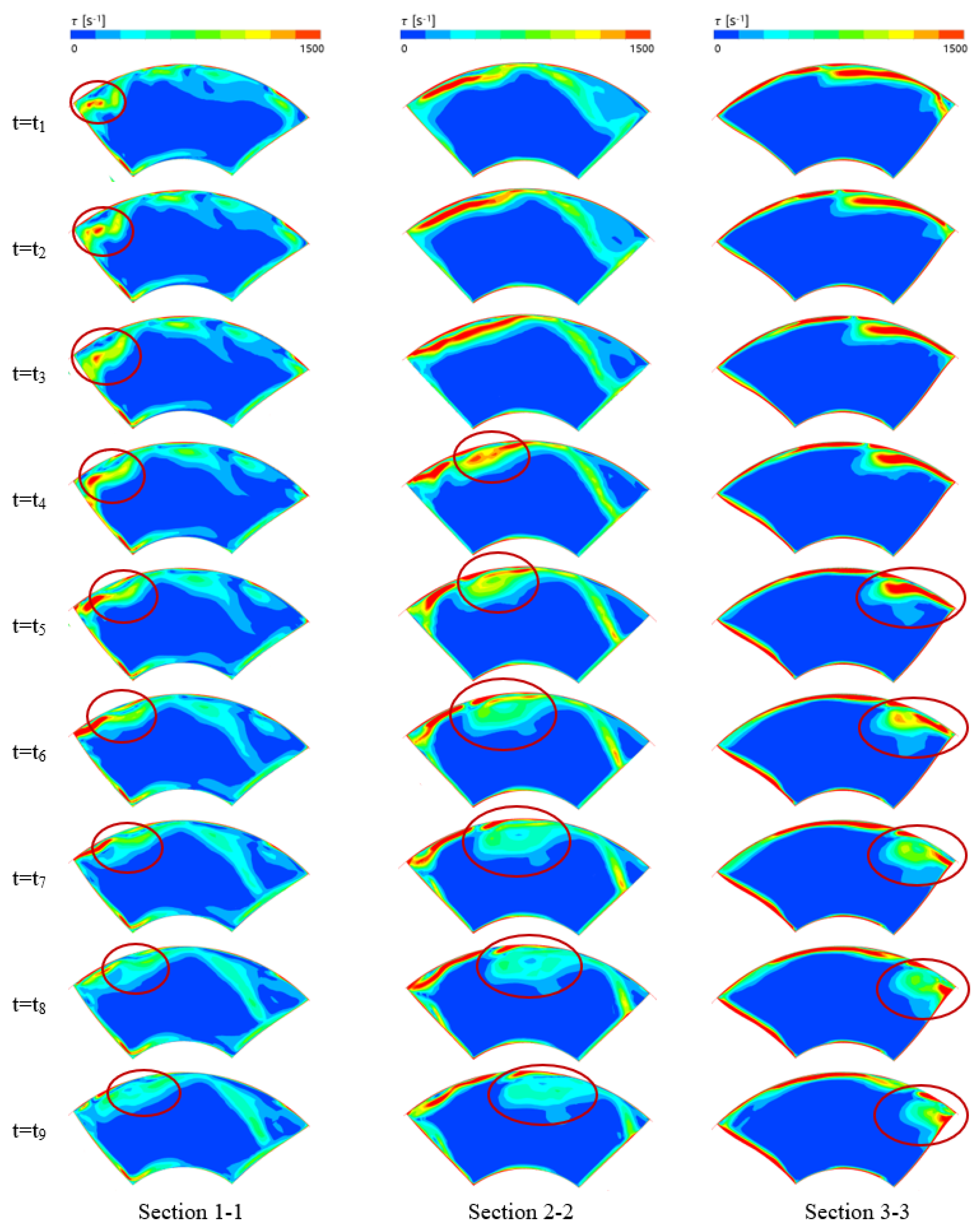
3.2.2. SSPCV Velocity Gradient

In order to explore the mechanism of SSPCV evolution, the velocity gradient of different sections was analyzed. The typical section is shown in Figure 12. Section 2-2 is the center surface of the impeller, and Section 1-1 and Section 3-3 are 0.02 m up and down from the center face, respectively. The velocity gradient is defined as

$$\tau =\sqrt{{\tau }_x^2+{\tau }_y^2}$$

(20)

$${\tau }_x=\mu \frac{dv}{dx},{\tau }_y=\mu \frac{du}{dy}$$

(21)

where ${\tau }_x$, ${\tau }_y$ is the velocity gradient in the x, y direction, m/s; and $u$, $v$ is the component of the absolute velocity in the x, y direction, m/s.

Figure 13 shows the variation of the velocity gradient of different typical sections. Due to the complex conditions of cavitation shedding and vortex, both cavitation and vortex produce velocity gradient. However, the velocity gradient generated by vortex is circular in scope and can be easily identified in the figure, so the main analysis area has been marked with red circles.

The Section 1-1 mainly shows the influence of blade tail on the velocity gradient. The vortex is generated from the tail of blade suction surface, and at this time cavitation is already in an unstable state. With the development of the vortex, the velocity gradient keeps increasing from t = t₁ to t = t₆, and reaches the maximum before the vortex enters the breaking stage. Then, it becomes elongated until it disappears.

Section 2-2 is the central plane, which has not been affected by vortex development from t = t₁ to t = t₃, so the long strip velocity gradient value formed by cavitation plays a major role. At time t = t₄, the vortex forms a stable structure. Under the influence of the vortex, the velocity gradient appears in a circular range, and the cavitation also curls along with the vortex. At this moment, the velocity gradient reaches its peak. Then, the range increases and the magnitude decreases. At t = t₉, the range is reduced compared with the last time, the influence generated by the vortex gradually dissipates, and the strip velocity gradient continues to extend, which means that the attached cavitation increases again.

The vortex stretches downwards, until t = t₅ does not affect the Section 3-3, the vortex has entered a stable stage. Therefore, the velocity gradient at this moment is the largest. Cavitation and vortex spin together and develop into a spiral structure. Due to the close distance to the next blade, it is affected by the next blade before full growth. From t = t₆, it enters the breaking stage, the vortex is cut by the blade, which accelerates the dissipation of the vortex.

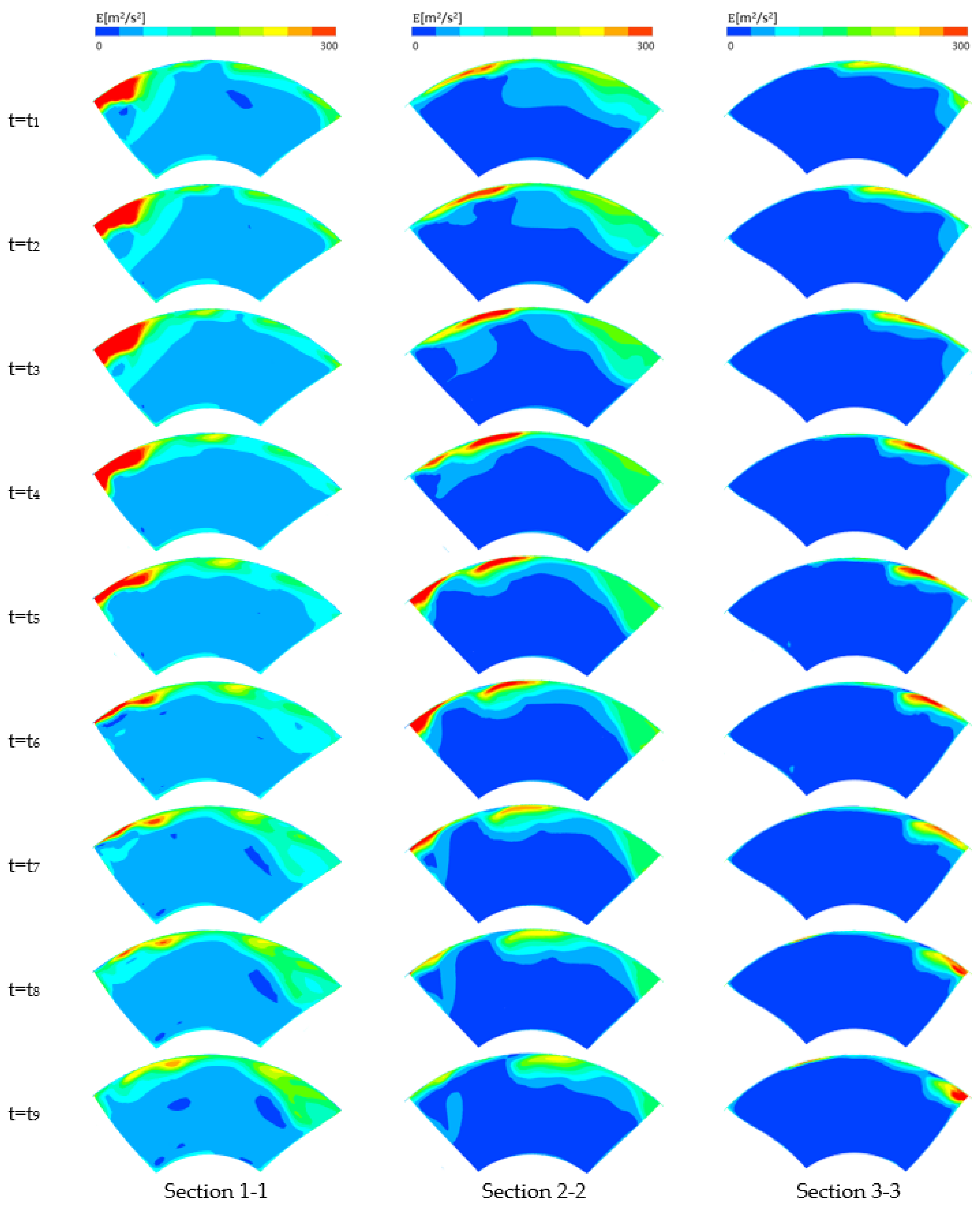
3.2.3. SSPCV Vortex Kinetic Energy

The kinetic energy of the vortex is defined as

$$E=\frac{1}{2}\left(u^2+v^2+w^2\right)$$

(22)

where, $w$ is the component of the absolute velocity in the z direction, m/s.

Figure 14 shows the changes of vortex kinetic energy of typical sections at different times. In Section 1-1, during the vortex formation stage from t = t₁ to t = t₃, the flow field is extremely chaotic, cavitation shedding is gradually formed, and small-scale vortices also appear gradually, so the vortex kinetic energy is flaked. The flow field is extremely chaotic, and the vortex kinetic energy appears as flakes. The maximum value appears at t = t₄, which is the early stage of the vortex development, and the vortex kinetic energy of the flake rapidly decreases with the development of the vortex from t = t₄ to t = t₅. The formation of SSPCV dissipates most of the energy. With the development of the vortex, the kinetic energy of the vortex decreases gradually, and the influence of the breaking stage on the section is not obvious. At Section 2-2, the kinetic energy of the vortex increases continuously during the formation stage of the vortex. Similarly, at t = t₄, the kinetic energy of the SSPCV reaches its maximum value, and from t = t₅ to t = t₉, the kinetic energy of the vortex decreases continuously. Compared with Section 1-1, in Section 2-2 the dissipation rate of the kinetic energy of the vortex is faster. The kinetic energy of the Section 3-3 vortex increases from t = t₁ to t = t₅, and reaches the maximum at t = t₅, which is slightly later than other sections, and is related to the downward stretching and development of the vortex. Then, the breaking stage begins. Before reaching the surface of the next blade, the kinetic energy of the vortex continues to decrease, and locally increases during the collision between the vortex and the blade wall from t = t₈ to t = t₉. In the breaking stage, only the vortex kinetic energy near the head of the next blade is significantly affected.

Before the SSPCV does not form a stable structure, the kinetic energy of the vortex is increasing, and the initial kinetic energy of the SSPCV is at its peak. Afterwards, due to the viscosity of the water, the energy of the vortex is continuously dissipated until the kinetic energy of the vortex is dissipated rapidly under the influence of the next blade. However, different sections have different performances. The dissipation rate of vortex energy in Section 1-1 is slow, followed by the dissipation rate in the center section. The vortex kinetic energy of the Section 3-3 is affected by the next blade and will increase locally.

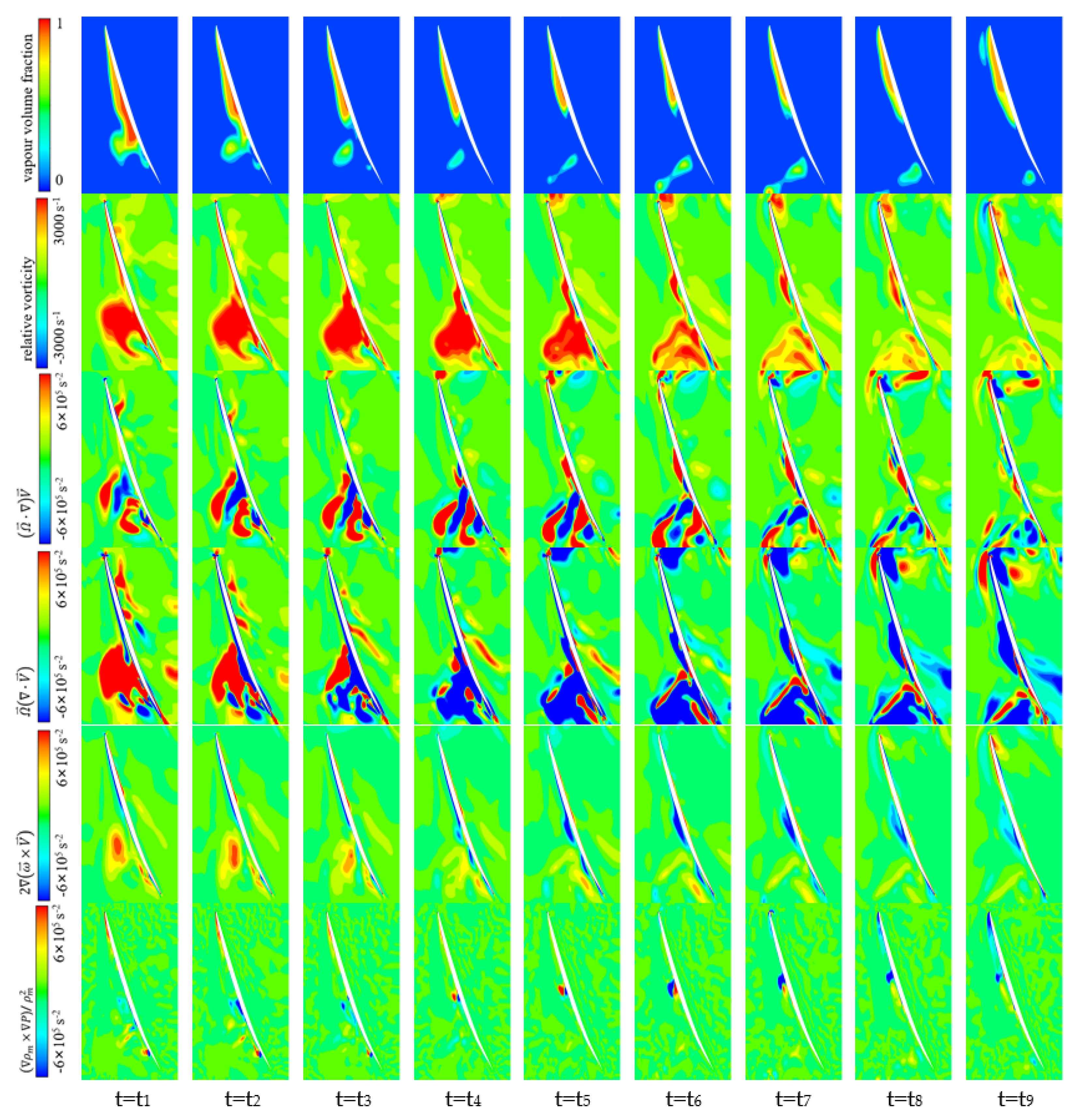
3.3. Vorticity Analysis in Impeller of Axial Flow Pump

In order to study the origins of vorticity, the vorticity transport equation (Equation (23)) is introduced to analyze the different typical moments in the cross-section of the impeller with span = 0.9, and the development laws of vorticity and each term are obtained.

$$\frac{D\stackrel{\rightharpoonup }{\Omega }}{Dt}=\left(\stackrel{\rightharpoonup }{\Omega }\cdot \nabla \right)\stackrel{\rightharpoonup }{V}-\stackrel{\rightharpoonup }{\Omega }\left(\nabla \cdot \stackrel{\rightharpoonup }{V}\right)-2\nabla \left(\stackrel{\rightharpoonup }{\omega }\times \stackrel{\rightharpoonup }{V}\right)+\frac{\nabla {\rho }_m\times \nabla P}{{\rho }_m^2}+\left(v_m+v_t\right){\nabla }^2\stackrel{\rightharpoonup }{\Omega }$$

(23)

where, $\stackrel{\rightharpoonup }{\omega }$ means the angular velocity, rad/s; $\stackrel{\rightharpoonup }{V}$ is relative velocity, m/s; $\stackrel{\rightharpoonup }{\Omega }$ is relative vorticity, s⁻¹; $v_m$ is kinematic viscosity, Pa·s; and $v_t$ is turbulence viscosity, Pa·s.

The left side of the equation represents the rate of change of vorticity, and the right side of the equation has five terms. The first term is the vortex stretching term, which describes the stretching and inclination of the vortex. The second vortex expansion term is related to velocity divergence. The third Coriolis force term is the virtual force which cannot be ignored in the rotating coordinate system. The fourth baroclinic moment term is related to the change of density. The fifth viscous diffusion term is related to the viscosity of the fluid and can be ignored at high Reynolds number flows.

Figure 15 shows the cloud images of the vapor volume fraction and vorticity transport equations at different times in the span = 0.9 direction of the impeller with the cavitation number σ = 0.18. The vapor volume fraction diagram mainly refers to the position of vorticity. In the state of deep cavitation, the flow in the tip area is complicated. Select span = 0.9 section for analysis.

Overall, vorticity is mainly generated in the shedding area of cloud cavitation. In terms of magnitude, the vortex stretching term and vortex expansion term contribute the most to vorticity. The Coriolis force is an influence factor that cannot be ignored in the rotating coordinate system. From the development of typical time, vorticity has a large value in both the vortex formation stage and development stage, but from the breaking stage (t = t₆) vorticity obviously decreases, and then quickly disappears. It shows that the influence of the next blade on the shedding vorticity is significant. The stretching term shows three phases of positive and negative. The center of the SSPCV is stretched longer, and the surroundings are also affected. It grows continuously from t = t₁ to t = t₅, and fracture occurs in the breaking stage, and then dissipates rapidly. From the formation stage to the development stage (t = t₁ to t = t₄), the expansion term appears positive and negative alternation. From the beginning of shedding, the fluid micelles expand in a large amount, forming cloud cavitation, and then rotating and evolving into the vortex in the development stage, and the cavitation core still shows expansion. After t = t₆ enters the breaking stage, there is no obvious change, indicating that the expansion term is not greatly affected by the next blade. The Coriolis force term is mainly concentrated in the range of suction-side-perpendicular cavitating vortex, but the magnitude is small. The baroclinic moment term has a large magnitude only at the vapor–liquid interface.

By comprehensive comparison, the most important factors affecting the vorticity are the stretching term and the expansion term. The vortex stretching term is the main contribution to the vorticity. The reason for the larger expansion term may be closely related to the cavitation number. The lower inlet pressure makes the fluid volume more susceptible to change and more sensitive to the influence of cavitation and vortices.

3.4. Method Comparison

The liutex method, vortex velocity gradient, vortex kinetic energy, and vorticity transport equation are used to analyze the evolution characteristics of SSPCV. The advantages and disadvantages of each method are as follows:

As a new type of vortex identification method, the liutex method can accurately identify the form of SSPCV, without wall pollution, and more intuitively and vividly display the evolution process of SSPCV. However, due to the adjustable threshold, the characteristics of SSPCV cannot be quantitatively displayed.

Vortex velocity gradient and vortex kinetic energy can quantify the vortex characteristics. Vortex velocity gradient shows the influence range of the vortex. The larger the velocity gradient, the greater the influence of the vortex. However, there are many reasons for the velocity gradient. Cavitation will also produce velocity gradient. Therefore, this method is vulnerable to other factors.

The vortex kinetic energy reflects the influence of the vortex from the energy point of view. The greater the energy of the vortex, the greater its hazard and the greater the impact on the performance of the pump. The vortex kinetic energy can quantify the harmfulness of the vortex.

The vorticity transport equation analyzes the origins of vorticity from the point of view of micelle, focusing on the internal mechanism of vortex. Compared with other methods, it is not intuitive and quantitative.

4. Conclusions

(1) The accuracy of SST-CC model is verified from two aspects of external characteristics and cavitation morphology, and the reliability of the analysis results is proven.

(2) The SSPCV is formed by the combined action of cloud cavitation shedding and tip leakage in the tip region, and its rotation direction is the same as that of the impeller. In the development process, it is continuously stretched into a slender structure until it is cut off by the next blade. In the process of cloud cavitation shedding, the turbulent kinetic energy is concentrated in the middle and rear of the hydrofoil, and the instantaneous turbulent kinetic energy of the flake cavitation retraction reaches the peak value, indicating that the turbulent intensity is greater in the middle and rear of the hydrofoil, which has a greater impact on the cavitation performance of the pump. The eddy viscosity is mainly concentrated on the head of the SSPCV, and the maximum can reach 1.5 Pa·s, indicating that the energy of the vortex is dissipated in the head.

(3) A new vortex identification method liutex is used to accurately identify the morphological evolution of SSPCV and have a more intuitive understanding of the structure of it. The evolution of vortex is analyzed by velocity gradient and vortex kinetic energy. The development of SSPCV is divided into three stages: formation, development, and breaking stage. At the beginning of the development stage, the velocity gradient is the largest, and the vortex kinetic energy is the largest and higher than 300 m²/s². With the development of vortex, the energy of the vortex continues to decay, and its range of influence continues to increase. The breaking stage can only affect the vortex in the local range of the blade head.

(4) By introducing the vorticity transport equation, the vortex stretching term and the vortex expansion term are the main contribution items of vorticity at low cavitation number, indicating that, under low flow rate and low cavitation number, the fluid micelles are prone to stretching expansion, and the deformation of the fluid micelle is the main cause of the vorticity. The Coriolis force term cannot be ignored in the rotating coordinate system. The breaking stage has a significant effect on vorticity; mainly the tensile deformation of the micelles is affected.

(5) The article still has some shortcomings, the quantitative description of the SSPCV is insufficient, and the data of pressure pulsation is lacking. Only the SSPCV with specific flow characteristics are analyzed without comparison.

References

1. Higashi, S.; Yoshida, Y.; Tsujimoto, Y. Tip leakage vortex cavitation from the tip clearance of a single hydrofoil. JSME Int. J. Ser. B-Fluids Therm. Eng. 2002, 45, 662–671. [Google Scholar] [CrossRef] [Green Version]
2. Coutier-Delgosha, O.; Stutz, B.; Vabre, A.; Legoupil, S. Analysis of cavitating flow structure by experimental and numerical investigations. J. Fluid Mech. 2007, 578, 171–222. [Google Scholar] [CrossRef] [Green Version]
3. Huang, B.; Young, Y.L.; Wang, G.; Shyy, W. Combined Experimental and Computational Investigation of Unsteady Structure of Sheet/Cloud Cavitation. J. Fluids Eng. Trans. ASME 2013, 135, 071301. [Google Scholar] [CrossRef]
4. Leroux, J.B.; Astolfi, J.A.; Billard, J.Y. An experimental study of unsteady partial cavitation. J. Fluids Eng. Trans. ASME 2004, 126, 94–101. [Google Scholar] [CrossRef]
5. Kadivar, E.; Timoshevskiy, M.V.; Pervunin, K.S.; el Moctar, O. Cavitation control using Cylindrical Cavitating-bubble Generators (CCGs): Experiments on a benchmark CAV2003 hydrofoil. Int. J. Multiph. Flow 2020, 125, 103186. [Google Scholar] [CrossRef]
6. Mejri, I.; Bakir, F.; Rey, R.; Belamri, T. Comparison of computational results obtained from a homogeneous cavitation model with experimental investigations of three inducers. J. Fluids Eng. Trans. ASME 2006, 128, 1308–1323. [Google Scholar] [CrossRef]
7. Lee, K.-H.; Yoo, J.-H.; Kang, S.-H. Experiments on cavitation instability of a two-bladed turbopump inducer. J. Mech. Sci. Technol. 2009, 23, 2350–2356. [Google Scholar] [CrossRef]
8. Choi, Y.-D.; Kurokawa, J.; Imamura, H. Suppression of cavitation in inducers by J-Grooves. J. Fluids Eng. Trans. ASME 2007, 129, 15–22. [Google Scholar] [CrossRef]
9. Bensow, R.E.; Bark, G. Implicit LES Predictions of the Cavitating Flow on a Propeller. J. Fluids Eng. Trans. ASME 2010, 132, 041302. [Google Scholar] [CrossRef]
10. Peters, A.; Lantermann, U.; el Moctar, O. Numerical prediction of cavitation erosion on a ship propeller in model- and full-scale. Wear 2018, 408, 1–12. [Google Scholar] [CrossRef]
11. Kumar, P.; Saini, R.P. Study of cavitation in hydro turbines-A review. Renew. Sustain. Energy Rev. 2010, 14, 374–383. [Google Scholar] [CrossRef]
12. Liu, Y.; Tan, L. Tip clearance on pressure fluctuation intensity and vortex characteristic of a mixed flow pump as turbine at pump mode. Renew. Energy 2018, 129, 606–615. [Google Scholar] [CrossRef]
13. Huang, R.; Ji, B.; Luo, X.; Zhai, Z.; Zhou, J. Numerical investigation of cavitation-vortex interaction in a mixed-flow waterjet pump. J. Mech. Sci. Technol. 2015, 29, 3707–3716. [Google Scholar] [CrossRef]
14. Guo, Q.; Huang, X.; Qiu, B. Numerical investigation of the blade tip leakage vortex cavitation in a waterjet pump. Ocean Eng. 2019, 187, 106170. [Google Scholar] [CrossRef]
15. Zhang, D.; Shi, W.; van Esch, B.P.M.; Shi, L.; Dubuisson, M. Numerical and experimental investigation of tip leakage vortex trajectory and dynamics in an axial flow pump. Comput. Fluids 2015, 112, 61–71. [Google Scholar] [CrossRef]
16. Shi, L.; Zhang, D.; Jin, Y.; Shi, W.; van Esch, B.P.M. A study on tip leakage vortex dynamics and cavitation in axial-flow pump. Fluid Dyn. Res. 2017, 49, 035504. [Google Scholar] [CrossRef]
17. Zhang, D.; Shi, W.; Pan, D.; Dubuisson, M. Numerical and Experimental Investigation of Tip Leakage Vortex Cavitation Patterns and Mechanisms in an Axial Flow Pump. J. Fluids Eng. Trans. ASME 2015, 137, 121103. [Google Scholar] [CrossRef]
18. Shen, X.; Zhang, D.; Xu, B.; Jin, Y.; Shi, W.; van Esch, B.P.M. Experimental Investigation of the Transient Patterns and Pressure Evolution of Tip Leakage Vortex and Induced-Vortices Cavitation in an Axial Flow Pump. J. Fluids Eng. Trans. ASME 2020, 142, 101206. [Google Scholar] [CrossRef]
19. Zhang, D.; Shi, L.; Shi, W.; Zhao, R.; Wang, H.; van Esch, B.P.M. Numerical analysis of unsteady tip leakage vortex cavitation cloud and unstable suction-side-perpendicular cavitating vortices in an axial flow pump. Int. J. Multiph. Flow 2015, 77, 244–259. [Google Scholar] [CrossRef]
20. Liu, C.; Gao, Y.S.; Dong, X.R.; Wang, Y.Q.; Liu, J.M.; Zhang, Y.N.; Cai, X.S.; Gui, N. Third generation of vortex identification methods: Omega and Liutex/Rortex based systems. J. Hydrodyn. 2019, 31, 205–223. [Google Scholar] [CrossRef]
21. Wang, Y.-Q.; Gao, Y.-S.; Liu, J.-M.; Liu, C. Explicit formula for the Liutex vector and physical meaning of vorticity based on the Liutex-Shear decomposition. J. Hydrodyn. 2019, 31, 464–474. [Google Scholar] [CrossRef]
Figure 1. High-precision test bench of Yangzhou University (1. inlet tank; 2. pump section and drive motor; 3. pressure outlet tank; 4. bifurcation tank; 5. condition regulating gate valve; 6. pressure stabilizing rectifier; 7. electromagnetic flowmeter; 8. forward and reverse operation control gate valve; 9. auxiliary pump unit; 10. differential pressure transmitter; and 11. absolute pressure transmitter).
Jmse 09 01058 g001
Figure 2. Model test physical objects and high-speed cameras.
Jmse 09 01058 g002
Figure 3. Overall size and grid of pump section.
Jmse 09 01058 g003
Figure 4. Impeller, guide vane and blade tip clearance grid.
Jmse 09 01058 g004
Figure 5. Wall YPlus value (left: pressure surface, middle: suction surface, and right: tip clearance).
Jmse 09 01058 g005
Figure 6. Analysis of Independence of Impeller Grid.
Jmse 09 01058 g006
Figure 7. Comparison of ησ between digital model and experiment.
Jmse 09 01058 g007
Figure 8. Comparison of ησ between numerical simulation and experiment.
Jmse 09 01058 g008
Figure 9. Evolution of cavitation patterns (top picture: experiment, bottom picture: numerical simulation).
Jmse 09 01058 g009
Figure 10. Span = 0.9 cavitation shedding and the evolution of turbulent kinetic energy.
Jmse 09 01058 g010
Figure 11. Liutex vortex recognition isosurface.
Jmse 09 01058 g011
Figure 12. Schematic diagram of different sections.
Jmse 09 01058 g012
Figure 13. Velocity gradient changes of typical cross-sections at different times.
Jmse 09 01058 g013
Figure 14. The vortex kinetic energy change of a typical section at different times.
Jmse 09 01058 g014
Figure 15. Various cloud diagrams of vapor volume fraction and vorticity transport equations for different span sections.
Jmse 09 01058 g015
Publisher’s Note: MDPI stays neutral with regard to jurisdictional claims in published maps and institutional affiliations.