Hydrodynamic Analysis and Motions of Ship with Forward Speed via a Three-Dimensional Time-Domain Panel Method

Abstract

A new three-dimensional (3D) time-domain panel method is developed to solve the ship hydrodynamic problem and motions. For an advancing ship with a constant forward speed in regular waves, the ship’s hull can be discretized and processed into a number of quadrilateral panels. Based on Green’s theorem, an analytical expression for Froude–Krylov (F–K) forces evaluation on the quadrilateral panels is derived without accuracy loss. Within the linear potential theory, the transient free surface Green function (TFSGF) is applied to solve the boundary value problem. To improve the efficiency and numerical stability of TFSGF evaluation, a precise integration method with variable parameters setting for extended identity matrix is developed to compute the TFSGF in the computation domain. Then, radiation and diffraction forces can be evaluated by means of the impulse response function method. The Wigley I hull form is taken as a study case, and the computed hydrodynamic coefficients, wave exciting forces, and motions by the present method are compared with previous literature experimental data and prior published results. It manifests that the three-dimensional time-domain panel method proposed in this paper has good accuracy.

1. Introduction

For the initial stages of ship design, accurate and reliable predictions of ship hydrodynamic analysis and motions in waves are essential. Various numerical methods are required to be developed for ship seakeeping analysis. For the wave-ship interaction problem with large size, the potential flow theory is much more efficient than RANS (Reynolds-averaged Navier-Stokes) simulation [1], which is widely applied to a practical engineering problem.

In the early researches, ship hydrodynamic analysis is developed based on two-dimensional strip theories. Ogilvie and Tuck [2], Tasai [3], and Salvesen et al. [4] proposed a new strip theory, rational strip theory, and STF, method respectively. The STF strip method is most widely used in ship motion calculation and structure design. Fonseca and Guedes Soares [5,6] formulated the ship hydrodynamic analysis in the time domain. Tavakoli et al. [7] investigated unsteady planning motion in waves using towing tank tests, Computational Fluid Dynamics (CFD), and the 2D+t model. These two-dimensional methods have been applied in the ship hydrodynamic and motion analysis for a long time. However, for the strip theories, the flow is assumed to be constrained in two-dimensional sections. Accurate hydrodynamic analysis can only be carried out for slender ships, and high frequency and low-speed assumptions are also required.

The shortcomings of strip theory can be overcome by 3D panel methods. Nakos [8] used the Rankine panel method to study the ship seakeeping problem in the frequency domain. Kring [9] and Chen [10] applied the Rankine panel method to ship hydrodynamic analysis in the time domain. The Rankine panel methods employ the Green function $1/r$ as a fundamental solution of the Laplace equation; the evaluation of $1/r$ integration over the boundaries is easy to be carried out. However, the Rankine Green function $1/r$ does not satisfy any boundary conditions, and many more panels are required for mesh discretization of the free surface, which would greatly reduce computational efficiency.

The problems caused by the Rankine panel method can be avoided by using the 3D free surface Green function method, which employs the 3D free surface Green function as the fundamental solution of the Laplace equation. The 3D free surface Green function method only requires the discretization of the ship wetted hull surface, but the evaluation of the 3D free surface Green function is quite complex. Wehausen and Laitone [11] deduced expressions for 3D free surface Green function in arbitrary water depth, which laid the foundation of solving the hydrodynamic problem by 3D free surface Green function method. Blandeau and Francois [12] solved the radiation and diffraction problem for FPSOs by using the HydroSTAR software, in which the original codes were developed by the frequency domain Green function method. Furthermore, Wu and Eatock Taylor [13] solved the hydrodynamic problem for practical ships by using the frequency domain Green function with speed. When the frequency domain Green function method is used to solve the ship hydrodynamic problems with speed, the numerical calculation of the frequency domain Green function is much more complex and time-consuming. Although the numerical results are close to the experimental values, there are still some problems in the treatment of waterline integral terms, which hinders its wide application. It’s easy to formulate and solve ship hydrodynamic problems and motion problems in the three-dimensional time domain. Liapis [14] applied the transient free surface Green function (TFSGF) to solve the linear radiation problem for a ship with constant forward speed. King [15] further extended to the linear diffraction problem for ships, and the Froude–Krylov (F–K) forces were evaluated by Gaussian quadrature. However, the F–K forces near the mean free surface may not be accurately evaluated due to wave volatility. Rodrigues and Guedes Soares [16] evaluated the Froude–Krylov forces by analytical exact pressure integration expressions, allowing for considerably coarse meshes with no loss of accuracy. However, radiation and diffraction forces are kept linear by the indirect time-domain method, which is difficult to calculate the hydrodynamic coefficients in the high-frequency range. Zhang et al. [17] studied the influences of the water line integral terms on the wave diffraction force of a moving floating body and pointed out that the influences of the water line integral terms on the first-order force could be ignored. Sun [18] developed a 3D time-domain program based on the TFSGF method, which can be used to solve the ship hydrodynamic problems in waves. Singh and Sen [19] studied seakeeping problems under different nonlinear levels, and computations were carried out for a Wigley hull and an S175 hull in waves. Datta et al. [20] carried out modifications for three fishing vessels and presented a variety of calculated motion results for different wave angles. Lin [21,22] proposed a three-dimensional time-domain approach to study the ship’s large-amplitude motions in a seaway and developed the software LAMP (Large Amplitude Motion Program) for ship hydrodynamic analysis and wave loads calculation.

The accurate and efficient evaluation of TFSGF is essential for the ship hydrodynamic analysis in the time domain. According to the oscillating properties of the wave part of TFSGF, King [15] and Shan [23] divided the time computation domain into different regions to evaluate the TFSGF and its derivatives, and series expansions and asymptotic expansions were applied to the small time computation domain and large time computation domain, respectively. Clement [24] firstly found that the TFSGF and its derivatives are the solutions of the ordinary differential equations (ODEs). Shen et al. [25] solved the ODEs by using the fourth-order Runge–Kutta method (RK44), in which the numerical instability would occur after a long time simulation even with a very small time step size. Based on the precise integration method (PIM) proposed by Zhong [26], Li et al. [27] solved the ODEs, which could greatly improve the numerical stability even with a quite large time step size. However, it can be very time-consuming due to the quite high order of the coefficient matrix.

Within the linear potential theory, the main objective of this paper is to develop a three-dimensional time-domain panel method to study the ship’s hydrodynamic analysis and motions. Analytical integration expressions for F–K force formulations over the quadrilateral panels can be derived by using Green’s theorem, which can avoid computational errors by numerical integration methods. To improve the accuracy and numerical stability of TFSGF evaluation, a numerical method is developed to solve the TFSGF by using a precise integration method with varying parameter settings. Based on the impulse response function method, the ship radiation problem and diffraction problem are solved by using TFSGF. The Wigley I hull is taken as a study case; convergence studies for ship hydrodynamic analysis and motions are conducted with respect to time step size and hull discretization. The computed hydrodynamic coefficients, wave exciting forces, and motions for the ship are compared to other solutions, such as Magee’s method [28], previous literature experimental data [29], and so on. Thus, the three-dimensional time-domain panel method proposed in this paper is validated.

2. Materials

2.1. Coordinate Systems

For the present linear ship hydrodynamic analysis and motion problem, as shown in Figure 1, a freely floating ship is considered to advance with constant forward speed U in the presence of a linear incident wave field. The $o\text{-}xyz$ is a reference, right-handed, Cartesian coordinate system with its origin o located amidship and travels along with the ship at the same speed U, the o-xy plane is coincident with the mean free surface z = 0, the positive x-axis is pointing upstream, the positive y-axis is pointing portside, and the positive z-axis is pointing vertically upwards. $G\text{-}{x}_{\mathrm{b}}{y}_{\mathrm{b}}{z}_{\mathrm{b}}$ is a body-fixed, right-handed, Cartesian coordinate system, and the origin G is located at the gravity of the ship. At initial time t = 0, the space fixed coordinate system $O\text{-}XYZ$ coincides with the reference coordinate system $o\text{-}xyz$, and $G{z}_{\mathrm{b}}$ axis is aligned with $ox$ axis. The fluid domain $\mathsf{\Omega }$ is enclosed by the ship hull surface $S_{\mathrm{B}}$, free surface $S_{\mathrm{F}}$, and surface $S_{\infty }$ at infinity. $n$ is the unit normal vector pointing inward the ship hull surface.

Figure 1. The coordinate systems and fluid domain.

2.2. Boundary Value Problem

Based on the linear potential flow theory, the fluid is assumed to be irrotational, inviscid, and incompressible, and there is no fluid separation or lifting effect [30]. In the reference coordinate system $o\text{-}xyz$, the total velocity potential $\mathsf{\Phi }\left(\mathit{r};t\right)$ in the infinite water can be written as

$$\mathsf{\Phi }\left(\mathit{r};t\right)=-Ux+{\mathsf{\Phi }}_{\mathrm{S}}\left(\mathit{r}\right)+{\mathsf{\Phi }}_0\left(\mathit{r};t\right)+{\displaystyle \sum _{k=1}^7{\mathsf{\Phi }}_k\left(\mathit{r};t\right)}$$

(1)

where $\mathit{r}=\left(x,y,z\right)$ is position vector on the ship hull surface, t is the time instant, $-Ux+{\mathsf{\Phi }}_{\mathrm{S}}\left(\mathit{r}\right)$ is the steady wave velocity potential due to constant forward speed U, ${\mathsf{\Phi }}_0$ is the incident wave velocity potential, ${\mathsf{\Phi }}_k\left(k=1,2,\cdots ,6\right)$ is radiation velocity potential, and ${\mathsf{\Phi }}_7$ is the diffraction velocity potential.

The perturbation potential ${\mathsf{\Phi }}_k$ (k = 1, 2, $\cdots$, 7) satisfies the following governing equations and initial-boundary value conditions:

$$\{\begin{array}{l}{\nabla }^2{\mathsf{\Phi }}_k\left(\mathit{r};t\right)=0,\mathrm{where}\mathit{r}\in \mathsf{\Omega }\\ \frac{{\partial }^2{\mathsf{\Phi }}_k}{\partial t^2}+\frac{\partial {\mathsf{\Phi }}_k}{\partial z}=0,\mathrm{on}z=0\\ \frac{\partial {\mathsf{\Phi }}_k}{\partial n}=m_k{\zeta }_k+n_k{\dot{\zeta }}_k,k=1,2,\cdots ,6,\mathrm{on}{S}_{\mathrm{B}}\\ \frac{\partial {\mathsf{\Phi }}_7}{\partial n}=-\frac{\partial {\mathsf{\Phi }}_0}{\partial n},\mathrm{on}{S}_{\mathrm{B}}\\ \nabla {\mathsf{\Phi }}_k\to 0,\mathrm{as}\sqrt{x^2+y^2}\to \infty \mathrm{or}z\to -\infty \\ {\mathsf{\Phi }}_k\mathrm{and}\frac{\partial {\mathsf{\Phi }}_k}{\partial t}\to 0,\mathrm{at}t=0,\left(k=1,2,\cdots ,6\right)\\ {\mathsf{\Phi }}_7\mathrm{and}\frac{\partial {\mathsf{\Phi }}_7}{\partial t}\to 0,\mathrm{at}t=-\infty .\end{array}$$

(2)

where ${\zeta }_k$ is unsteady motion in the kth mode; $n=\left(n_1,n_2,n_3\right)$; $\mathit{r}\times n=\left(n_4,n_5,n_6\right)$; $\left(m_1,m_2,m_3\right)=\left(0,0,0\right)$; $\left(m_4,m_5,m_6\right)=\left(0,U{n}_3,-U{n}_2\right)$; g is the gravity acceleration [31].

The TFSGF is adopted to solve the boundary value problem and written as [14]

$$G\left(P,Q;t-\tau \right)=\overline{G}\left(P;Q\right)\delta \left(t-\tau \right)+\tilde{G}\left(P,Q;t-\tau \right)H\left(t-\tau \right)$$

(3)

where $\delta (·)$ is the Dirac function; $H(·)$ is Heaviside unit step function; P(x, y, z) is field point; Q(ξ, η, ζ) is source point; $\tau$ is the retard time. The Rankine part $\overline{G}\left(P;Q\right)$ and memory part $\tilde{G}\left(P,Q;t-\tau \right)$ of $G\left(P,Q;t-\tau \right)$ can be given as

$$\{\begin{array}{l}\overline{G}\left(P,Q\right)=1/r-1/r^{\prime }\\ \tilde{G}\left(P,Q;t-\tau \right)=2{\displaystyle {\int }_0^{\infty }\sqrt{g\upsilon }{\mathrm{e}}^{\upsilon \left(z+\zeta \right)}\sin \left[\sqrt{g\upsilon }\left(t-\tau \right)\right]{\mathrm{J}}_0\left(\upsilon R\right)\mathrm{d}\upsilon }\end{array}$$

(4)

where $r=\left|P-Q\right|$; $r^{\prime }=\left|P-Q^{\prime }\right|$; $Q^{\prime }\left(\xi ,\eta ,-\zeta \right)$ is the image point of Q about the mean free surface; R is the horizontal distance between the field point P and source point Q; ${\mathrm{J}}_0$ is a Bessel function of order zero; $\upsilon$ is wave number.

The integrations for $\overline{G}$ and its derivative over a quadrilateral panel can be computed by Hess–Smith method [32]. $\tilde{G}$ and its derivatives can be solved numerically in Section 3.2.

The boundary integral equation for the perturbation potential ${\mathsf{\Phi }}_k$ (k = 1, 2, $\cdots$, 7) can be written as

$$\begin{array}{l}2\mathsf{\pi }{\mathsf{\Phi }}_k\left(P;t\right)+{\displaystyle {\iint }_{S_{\mathrm{B}}}{\mathsf{\Phi }}_k\left(Q;t\right)\frac{\partial \overline{G}}{\partial n_Q}\mathrm{d}{S}_Q}={\displaystyle {\iint }_{S_{\mathrm{B}}}\overline{G}\frac{\partial {\mathsf{\Phi }}_k\left(Q;t\right)}{\partial n_Q}\mathrm{d}S}\\ +{\displaystyle {\int }_{t_0}^t\mathrm{d}\tau }{\displaystyle {\iint }_{S_{\mathrm{B}}}\tilde{G}\left(P,Q;t-\tau \right)\frac{\partial {\mathsf{\Phi }}_k\left(Q;\tau \right)}{\partial n_Q}\mathrm{d}S}-{\displaystyle {\int }_{t_0}^t\mathrm{d}\tau }{\displaystyle {\iint }_{S_{\mathrm{B}}}{\mathsf{\Phi }}_k\left(Q,\tau \right)\frac{\partial \tilde{G}\left(P,Q;t-\tau \right)}{\partial n_Q}\mathrm{d}S}\\ +\frac{U^2}{g}{\displaystyle {\int }_{t_0}^t\mathrm{d}\tau }{\displaystyle {\oint }_{{\Gamma }_0}\tilde{G}\left(P,Q;t-\tau \right)\frac{\partial {\mathsf{\Phi }}_k\left(Q;\tau \right)}{\partial \xi }\mathrm{d}\eta }-\frac{U^2}{g}{\displaystyle {\int }_{t_0}^t\mathrm{d}\tau }{\displaystyle {\oint }_{{\Gamma }_0}{\mathsf{\Phi }}_k\left(Q;\tau \right)\frac{\partial \tilde{G}\left(P,Q;t-\tau \right)}{\partial \xi }\mathrm{d}\eta }\\ +\frac{2U}{g}{\displaystyle {\int }_{t_0}^t\mathrm{d}\tau }{\displaystyle {\oint }_{{\Gamma }_0}{\mathsf{\Phi }}_k\left(Q;\tau \right)\frac{\partial \tilde{G}\left(P,Q;t-\tau \right)}{\partial \tau }\mathrm{d}\eta }\end{array}$$

(5)

where ${\Gamma }_0$ is the mean waterline; $t_0$ is the initial time; $n_Q$ is the unit normal vector of source point Q pointing inward the hull surface.

To solve the perturbation potential ${\mathsf{\Phi }}_k$, the trapezoidal rule is adopted for convolution integration, and the mean wet hull surface $S_{\mathrm{B}}$ in Equation (5) can be discretized by using the constant panel method [31].

2.3. The Hydrodynamic Problem Formulation

Based on the impulse response function method, the radiation potential ${\mathsf{\Phi }}_k$ ($k=1,2,\cdots ,6$) can be written as

$${\mathsf{\Phi }}_k\left(P;t\right)={\displaystyle {\int }_0^t{\widehat{\mathsf{\Phi }}}_k\left(P;t-\tau \right){\dot{\zeta }}_k\left(\tau \right)\mathrm{d}\tau }$$

(6)

where ${\widehat{\mathsf{\Phi }}}_k\left(P;t\right)$ is the impulse response function of radiation potential ${\mathsf{\Phi }}_k$ in the kth mode.

The ${\widehat{\mathsf{\Phi }}}_k\left(P;t\right)$ can be decomposed into the following form [14]

$${\widehat{\mathsf{\Phi }}}_k\left(P;t\right)={\psi }_{1k}\left(P\right)\delta \left(t\right)+{\psi }_{2k}\left(P\right)H\left(t\right)+{\chi }_k\left(P;t\right)$$

(7)

where ${\psi }_{1k}$ and ${\psi }_{2k}$ are the impulsive potentials, and ${\chi }_k$ is the transient potential.

The expression of radiation forces $F_{jk}$ can be written as

$$F_{jk}\left(t\right)=-a_{jk}{\ddot{\zeta }}_k\left(t\right)-b_{jk}{\dot{\zeta }}_k\left(t\right)-c_{jk}{\zeta }_k\left(t\right)-{\displaystyle {\int }_0^t\mathrm{d}\tau }{K}_{jk}\left(t-\tau \right){\dot{\zeta }}_k\left(\tau \right)$$

(8)

where $F_{jk}$ is the radiation force in jth mode due to kth mode motion; $K_{jk}\left(t\right)=\rho {\displaystyle {\iint }_{S_{\mathrm{B}}}\left(\frac{\partial {\chi }_k}{\partial t}{n}_j-{\chi }_k{m}_j\right)\mathrm{d}S}$; $a_{jk}=-\rho {\displaystyle {\iint }_{S_{\mathrm{B}}}{\psi }_{1k}{n}_j\mathrm{d}S}$; $c_{jk}=-\rho {\displaystyle {\iint }_{S_{\mathrm{B}}}{\psi }_{2k}{m}_j\mathrm{d}S}$; $b_{jk}=-\rho {\displaystyle {\iint }_{S_{\mathrm{B}}}\left({\psi }_{2k}{n}_j-{\psi }_{1k}{m}_j\right)\mathrm{d}S}$.

The added mass $A_{jk}\left(\omega \right)$ and damping coefficients $B_{jk}\left(\omega \right)$ can be obtained via Fourier transform ($j=1,2,\cdots ,6$; $k=1,2,\cdots ,6$) [15]:

$$\{\begin{array}{l}{A}_{jk}\left(\omega \right)=a_{jk}-\frac{c_{jk}}{{\omega }^2}-\frac{1}{\omega }{\displaystyle {\int }_0^{\infty }{K}_{jk}\left(\tau \right)\sin \left(\omega \tau \right)\mathrm{d}\tau }\\ B_{jk}\left(\omega \right)=b_{jk}+{\displaystyle {\int }_0^{\infty }{K}_{jk}\left(\tau \right)\cos \left(\omega \tau \right)\mathrm{d}\tau }\end{array}$$

(9)

In the infinite water depth, the analytical expression of linear incident wave potential ${\mathsf{\Phi }}_{\mathrm{I}}\left(P;t\right)$ in the reference coordinate system $o\text{-}xyz$ can be given as [31]

$${\mathsf{\Phi }}_{\mathrm{I}}\left(P;t\right)=\frac{\mathrm{i}{\eta }_{0}g}{\omega }{\mathrm{e}}^{\upsilon \left[z-\mathrm{i}\left(x\cos \alpha +y\sin \alpha \right)\right]}{\mathrm{e}}^{\mathrm{i}{\underset{\dot{}}{\omega }}_{\mathrm{e}}t}$$

(10)

where ${\eta }_0$ is the amplitude of incident wave; $\alpha$ is wave propagation angle ($\alpha =\mathsf{\pi }$ is head waves); $\omega$ is the absolute frequency; $\upsilon ={\omega }^2/g$; ${\omega }_{\mathrm{e}}=\omega -\upsilon U\cos \alpha$ is the encounter frequency.

The elevation ${\eta }_{\mathrm{I}}\left(t\right)$ of the incident wave at the origin o is given as

$${\eta }_{\mathrm{I}}\left(t\right)={\eta }_0{\mathrm{e}}^{\mathrm{i}{\omega }_{\mathrm{e}}t}$$

(11)

Based on the impulse response function method [10], the incident wave velocity $\nabla {\mathsf{\Phi }}_{\mathrm{I}}\left(P;t\right)$, diffraction velocity potential ${\mathsf{\Phi }}_7\left(P;t\right)$, and the diffraction force $F_{j7}\left(t\right)$ in the jth mode ($j=1,2,\cdots ,6$), $\widehat{K}\left(P;t\right)$, ${\widehat{\mathsf{\Phi }}}_7\left(P;t\right)$, and $K_{j7}\left(t\right)$ can be expressed in the following as

$$\{\begin{array}{l}\nabla {\mathsf{\Phi }}_{\mathrm{I}}\left(P;t\right)={\displaystyle {\int }_{-\infty }^{\infty }\widehat{K}\left(P;t-\tau \right){\eta }_{\mathrm{I}}\left(\tau \right)\mathrm{d}\tau }\\ {\mathsf{\Phi }}_7\left(P;t\right)={\displaystyle {\int }_{-\infty }^{\infty }{\widehat{\mathsf{\Phi }}}_7\left(P;t-\tau \right){\eta }_{\mathrm{I}}\left(\tau \right)\mathrm{d}\tau }\\ F_{j7}\left(t\right)={\displaystyle {\int }_{-\infty }^{\infty }{K}_{j7}\left(t-\tau \right){\eta }_{\mathrm{I}}\left(\tau \right)\mathrm{d}\tau }\end{array}$$

(12)

where $\widehat{K}\left(P;t\right)$ is the impulse response function of incident wave velocity $\nabla {\mathsf{\Phi }}_{\mathrm{I}}\left(P;t\right)$, ${\widehat{\mathsf{\Phi }}}_7\left(P;t\right)$ is the impulse response function of ${\mathsf{\Phi }}_7\left(P;t\right)$, and $K_{j7}\left(t\right)$ is the impulse response function of $F_{j7}\left(t\right)$.

In combination with Equations (2), (5) and (12), the $K_{j7}\left(t\right)$ is given by

$$K_{j7}\left(t\right)={\displaystyle {\iint }_{S_{\mathrm{B}}}\rho \left[{\widehat{\mathsf{\Phi }}}_7\left(P;t\right)m_j-n_j\frac{\partial {\widehat{\mathsf{\Phi }}}_7\left(P;t\right)}{\partial t}\right]\mathrm{d}S}$$

(13)

2.4. Solving the Ship Motion Equations

Using Newton’s second law, the six degree of freedom motions of the rigid body in space fixed coordinate system are determined by

$$M_{ij}\left\{{\ddot{\zeta }}_j\left(t\right)\right\}=F_i\left(t\right)$$

(14)

where $F_i\left(t\right)=F_{i\mathrm{I}}\left(t\right)+F_{i\mathrm{H}}\left(t\right)+F_{i7}\left(t\right)+{\displaystyle \sum _{j=1}^6{F}_{ij}\left(t\right)}$, $F_{i\mathrm{I}}\left(t\right)$ is F–K forces in the ith mode, $F_{i\mathrm{H}}\left(t\right)$ is hydrostatic forces in the ith mode, and $M_{ij}$ is the element of the general mass matrix.

In the body coordinate system $G\text{-}{x}_{\mathrm{b}}{y}_{\mathrm{b}}{z}_{\mathrm{b}}$, the six-degrees of motion equation can also be given as

$$\mathit{m}\dot{\mathit{u}}+\mathit{m}\mathit{\Lambda }\times \mathit{u}={\mathit{F}}_{\mathrm{b}};\mathit{I}\dot{\mathit{\Lambda }}+\mathit{\Lambda }\times \mathit{I}\mathit{\Lambda }={\mathit{M}}_{\mathrm{b}}$$

(15)

where $m$ is the mass matrix, $I$ is inertial moment matrix, $u=\left(u,v,w\right)$ is velocity vector, $\Lambda =\left({\Lambda }_{x_{\mathrm{b}}},{\Lambda }_{y_{\mathrm{b}}},{\Lambda }_{z_{\mathrm{b}}}\right)$ is the angular velocity, $F_{\mathrm{b}}=\left(F_{x_{\mathrm{b}}},F_{y_{\mathrm{b}}},F_{z_{\mathrm{b}}}\right)$ is force vector, and $M_{\mathrm{b}}=\left(M_{x_{\mathrm{b}}},M_{y_{\mathrm{b}}},M_{z_{\mathrm{b}}}\right)$ is moment vector.

The vectors between the space fixed coordinate system and the body coordinate system can be transformed by a transformation matrix [33]. For linear problems, the transformation matrix is the identity matrix.

The ship motion equations can be solved by various numerical methods, such as Runge–Kutta method, predictor-correctors method, and so on. To avoid initial numerical instability, a ramp function [34] is applied to solve the ship motion equations.

3. Numerical Methods

3.1. Analytical Expression for F–K Forces Evaluation

Consider two coordinate systems illustrated in Figure 2: the reference coordinate system o-xyz and the local panel coordinate system $o^{\prime }\text{-}{x}^{\prime }{y}^{\prime }{z}^{\prime }$ defined by the vertices 1 to 4 in the counterclockwise direction, named $P_1$, $P_2$, $P_3$, and $P_4$, respectively. The positive $o^{\prime }{z}^{\prime }$ axis points to the exterior of the fluid.

Figure 2. The reference coordinate system o-xyz and local panel coordinate system $o^{\prime }\text{-}{x}^{\prime }{y}^{\prime }{z}^{\prime }$.

The transformation matrix between the position vector $\mathit{r}$ in the reference coordinate system $oxyz$ and the position vector ${\mathit{r}}^{\prime }$ in the local panel coordinate system $o^{\prime }\text{-}{x}^{\prime }{y}^{\prime }{z}^{\prime }$ is given as

$$\mathit{r}={\mathit{r}}_0+\mathit{T}{\mathit{r}}^{\prime }$$

(16)

where ${\mathit{r}}_o=\left(x_o,y_o,z_o\right)$ is the position vector in $o\text{-}xyz$, which is the origin of the panel coordinate $o^{\prime }\text{-}{x}^{\prime }{y}^{\prime }{z}^{\prime }$ system, $T$ is the unit transformation cosine-director matrix between system $o^{\prime }\text{-}{x}^{\prime }{y}^{\prime }{z}^{\prime }$ and system $o\text{-}xyz$ and given by

$$T=\left[\begin{array}{ccc}⟨x^{\prime },x⟩& ⟨y^{\prime },x⟩& ⟨z^{\prime },x⟩\\ ⟨x^{\prime },y⟩& ⟨y^{\prime },y⟩& ⟨z^{\prime },y⟩\\ ⟨x^{\prime },z⟩& ⟨y^{\prime },z⟩& ⟨z^{\prime },z⟩\end{array}\right]$$

(17)

where $x$, $y$, and $z$ are unit base vectors in system $o\text{-}xyz$; $x^{\prime }$, $y^{\prime }$, and $z^{\prime }$ are unit base vectors in system $o\text{-}{x}^{\prime }{y}^{\prime }{z}^{\prime }$; $⟨,⟩$ denotes the internal product between base vectors.

Within linear dynamic conditions, the elevation ${\eta }_{\mathrm{I}}\left(t\right)$ $\left(z\le 0\right)$ is given as

$$\{\begin{array}{l}{p}_{\mathrm{I}}\left(t\right)=\rho g{\eta }_0{\mathrm{e}}^{\upsilon z}\cos \left[{\omega }_{\mathrm{e}}t-\upsilon \left(x\cos \alpha +y\sin \alpha \right)\right]\\ p_{\mathrm{H}}=-\rho gz\end{array}$$

(18)

The pressure $p_{\mathrm{IH}}$ can be given by

$$p_{\mathrm{IH}}=\rho g{\eta }_{\mathrm{I}}\left(t\right){\mathrm{e}}^{\upsilon z}-\rho gz$$

(19)

The resultant forces of F–K forces and hydrostatic forces acting on the mean wetted hull surface in the jth mode can be given by

$$F_{\mathrm{IH}j}\left(t\right)={\displaystyle {\iint }_{S_{\mathrm{B}}}{p}_{\mathrm{IH}}\left(t\right)n_j\mathrm{d}S}$$

(20)

The mean wetted hull surface can be discretized by $N$ quadrilateral panels. For the ith quadrilateral panel under the mean free surface, the F–K force $F_{\mathrm{I}i}$ can be written as

$$F_{\mathrm{I}i}=n_i\rho g{\eta }_0{\displaystyle {\iint }_{S_i}{\mathrm{e}}^{\upsilon z}\cos \left[{\omega }_{\mathrm{e}}t-\upsilon \left(x\cos \alpha +y\sin \alpha \right)\right]\mathrm{d}S}$$

(21)

where $n_i$ is the unit normal vector pointing outward the fluid, and $S_i$ is the area of the quadrilateral panel.

The Equation (21) can be represented in the ith local panel coordinate system $o^{\prime }\text{-}{x}^{\prime }{y}^{\prime }{z}^{\prime }$

$$F_{\mathrm{I}i}=n_i\rho g{\eta }_0{\displaystyle {\iint }_{S_i}{\mathrm{e}}^{\mathrm{B}\left(x^{\prime },y^{\prime }\right)}\cos \mathrm{A}\left(x^{\prime },y^{\prime }\right)\mathrm{d}S}$$

(22)

where $\mathrm{A}\left(x^{\prime },y^{\prime }\right)={\omega }_{\mathrm{e}}t-\upsilon \left[\left(x_o+⟨x^{\prime },x⟩x^{\prime }+⟨y^{\prime },x⟩y^{\prime }\right)\cos \alpha +\left(y_o+⟨x^{\prime },y⟩x^{\prime }+⟨y^{\prime },y⟩y^{\prime }\right)\sin \alpha \right]$, and $\mathrm{B}\left(x^{\prime },y^{\prime }\right)=\upsilon \left(z_o+⟨x^{\prime },z⟩x^{\prime }+⟨y^{\prime },z⟩y^{\prime }\right)$.

The jth $\left(j=1,2,3,4\right)$ edge for the ith quadrilateral panel can be parametrized by

$$g_{ij}\left(\kappa \right)=\left({x^{\prime }}_{0,ij},{y^{\prime }}_{0,ij}\right)+\left(\Delta {x^{\prime }}_{ij},\Delta {y^{\prime }}_{ij}\right)\kappa ,\kappa \in \left[0,1\right]$$

(23)

where $\Delta {x^{\prime }}_{ij}={x^{\prime }}_{1,ij}-{x^{\prime }}_{0,ij}$, $\Delta {y^{\prime }}_{ij}={y^{\prime }}_{1,ij}-{y^{\prime }}_{0,ij}$, ${x^{\prime }}_{0,ij}={x^{\prime }}_{ij}\left(0\right)$; ${x^{\prime }}_{1,ij}={x^{\prime }}_{ij}\left(1\right)$, ${y^{\prime }}_{0,ij}={y^{\prime }}_{ij}\left(0\right)$, and ${y^{\prime }}_{1,ij}={y^{\prime }}_{ij}\left(1\right)$.

$\mathrm{A}$, $\mathrm{B}$, and their derivatives on the jth side of the ith panel can be expressed with respect to parameter $\kappa$ as

$$\{\begin{array}{l}{\mathrm{A}}_{ij}\left(\kappa \right)={\omega }_{\mathrm{e}}t-\upsilon \left\{\left[\begin{array}{l}\left[x_o+⟨x^{\prime },x⟩\left({x^{\prime }}_{0,ij}+\Delta {x^{\prime }}_{ij}\kappa \right)+⟨y^{\prime },x⟩\left({y^{\prime }}_{0,ij}+\Delta {y^{\prime }}_{ij}\kappa \right)\right]\cos \alpha \\ +\left[y_o+⟨x^{\prime },y⟩\left({x^{\prime }}_{0,ij}+\Delta {x^{\prime }}_{ij}\kappa \right)+⟨y^{\prime },x⟩\left({y^{\prime }}_{0,ij}+\Delta {y^{\prime }}_{ij}\kappa \right)\right]\sin \alpha \end{array}\right]\right\}\\ {\mathrm{B}}_{ij}\left(\kappa \right)=\upsilon \left[z_o+⟨x^{\prime },z⟩\left({x^{\prime }}_{0,ij}+\Delta {x^{\prime }}_{ij}\kappa \right)+⟨y^{\ast },z⟩\left({y^{\prime }}_{0,ij}+\Delta {y^{\prime }}_{ij}\kappa \right)\right]\end{array}$$

(24)

Let ${\mathsf{\Psi }}_{\kappa }={\mathrm{A}}_{\kappa }^2+{\mathrm{B}}_{\kappa }^2$, and

$$CE=\{\begin{array}{l}\frac{{\mathrm{e}}^{\mathrm{B}}\left({\mathrm{B}}_{\kappa }\cos \mathrm{A}+{\mathrm{A}}_{\kappa }\sin \mathrm{A}\right)}{{\mathsf{\Psi }}_{\kappa }},{\mathsf{\Psi }}_{\kappa }\ne 0\\ {\mathrm{e}}^{\mathrm{B}}\kappa \cos \mathrm{A},{\mathsf{\Psi }}_{\kappa }=0\end{array}$$

(25)

$$SE=\{\begin{array}{l}\frac{{\mathrm{e}}^{\mathrm{B}}\left({\mathrm{B}}_{\kappa }\sin \mathrm{A}-{\mathrm{A}}_{\kappa }\cos \mathrm{A}\right)}{{\mathsf{\Psi }}_{\kappa }},{\mathsf{\Psi }}_{\kappa }\ne 0\\ {\mathrm{e}}^{\mathrm{B}}\kappa \sin \mathrm{A},{\mathsf{\Psi }}_{\kappa }=0\end{array}$$

(26)

With respect to parameter $\kappa$, $\mathrm{A}$ and $\mathrm{B}$’s derivatives on the ith panel are written as

$$\{\begin{array}{l}{\mathrm{A}}_{x^{\prime },i}=-\upsilon \left(⟨x^{\prime },x⟩\cos \alpha +⟨x^{\prime },y⟩\sin \alpha \right)\\ {\mathrm{A}}_{y^{\prime },i}=-\upsilon \left(⟨y^{\prime },x⟩\cos \alpha +⟨y^{\prime },y⟩\sin \alpha \right)\\ {\mathrm{B}}_{x^{\prime },i}=\upsilon ⟨x^{\prime },z⟩,{\mathrm{B}}_{y^{\prime },i}=\upsilon ⟨y^{\prime },z⟩\end{array}$$

(27)

Let ${\mathsf{\Psi }}_{x^{\prime }}={\mathrm{A}}_{x^{\prime }}^2+{\mathrm{B}}_{x^{\prime }}^2$ and ${\mathsf{\Psi }}_{y^{\prime }}={\mathrm{A}}_{y^{\prime }}^2+{\mathrm{B}}_{y^{\prime }}^2$. The Green’s theorem with parameterization in Equation (23) is applied, and integration by parts is adopted to solve Equation (22). If ${\mathsf{\Psi }}_{x^{\prime }}\ne 0$, Equation (22) is expressed as

$$F_{\mathrm{I}i}=\frac{n_i\rho g{\eta }_0}{{\mathsf{\Psi }}_{x^{\prime }}}{\displaystyle \sum _{j=1}^4\Delta y_{ij}^{\prime }{\displaystyle {\int }_0^1{\mathrm{e}}^{{\mathrm{B}}_{ij}\left(\kappa \right)}\left[{\mathrm{B}}_{x^{\prime },i}\cos {\mathrm{A}}_{ij}\left(\kappa \right)+{\mathrm{A}}_{x^{\prime },i}\sin {\mathrm{A}}_{ij}\left(\kappa \right)\right]\mathrm{d}\kappa }}$$

(28)

$\Delta C{E}_{ij}$ can be understood as $\left[C{E}_{ij}\left(1\right)-C{E}_{ij}\left(0\right)\right]$, and $\Delta S{E}_{ij}$ can be understood as $\left[S{E}_{ij}\left(1\right)-S{E}_{ij}\left(0\right)\right]$. $F_{\mathrm{I}i}$ is written as

$$F_{\mathrm{I}i}=\frac{n_i\rho g{\eta }_0}{{\mathsf{\Psi }}_{x^{\prime }}}{\displaystyle \sum _{j=1}^4\Delta y_{ij}^{\ast }\left({\mathrm{B}}_{x^{\prime },i}\Delta C{E}_{ij}+{\mathrm{A}}_{x^{\prime },i}\Delta S{E}_{ij}\right)}$$

(29)

If ${\mathsf{\Psi }}_{y^{\prime }}\ne 0$, $F_{\mathrm{I}i}$ is directly solved by

$$F_{\mathrm{I}i}=\frac{-n_i\rho g{\eta }_0}{{\mathsf{\Psi }}_{y^{\prime }}}{\displaystyle \sum _{j=1}^4\Delta x_{ij}^{\prime }\left({\mathrm{B}}_{y^{\prime },i}\Delta C{E}_{ij}+{\mathrm{A}}_{y^{\prime },i}\Delta S{E}_{ij}\right)}$$

(30)

Note that the analytical integration expressions for F–K moments, hydrostatic forces, and hydrostatic moments can be solved in a similar approach.

With the established formulation for F–K forces evaluation, it is worth comparing the present method with the method proposed by Rodrigues and Guedes Soares (2017) [16] (see Table 1).

Table 1. Differences between the present method and Rodrigues’s method.

	Present Method	Rodrigues’s Method [16]
Equation of motion	Froude–Krylov forces calculated and motions solved in a moving system fixed to the ship.	Froude–Krylov forces calculated in an inertial frame, and motions solved in a moving system fixed to the ship.
Ship velocity	arbitrary	zero
Diffraction force	direct time-domain method	indirect time-domain method
Radiation force	direct time-domain method	indirect time-domain method
Expression of incident wave elevation	cosine form	sinusoidal form

3.2. Numerical Method for TFSGF Evaluation

The memory part of TFSGF in Equation (4) can be written in the non-dimensional form

$$\tilde{G}\left(P,Q;t-\tau \right)=2\sqrt{g/{{\mathit{r}}^{\prime }}^3}F\left(\mu ,\beta \right)$$

(31)

where $\nu =\upsilon r^{\prime }$, $\mu =-\left(z+\zeta \right)/r^{\prime }$, and $\beta =\sqrt{g/r^{\prime }}\left(t-\tau \right)$. $F\left(\mu ,\beta \right)$ is given by

$$F\left(\mu ,\beta \right)={\displaystyle {\int }_0^{\infty }\sqrt{\nu }\sin \left(\beta \sqrt{\nu }\right){\mathrm{e}}^{-\nu \mu }{\mathrm{J}}_0\left(\nu \sqrt{1-{\mu }^2}\right)\mathrm{d}\nu }$$

(32)

$F\left(\mu ,\beta \right)$ is the solution to the following fourth-order ODE

$$\frac{{\partial }^{4}F\left(\mu ,\beta \right)}{\partial {\beta }^4}+\mu \beta \frac{{\partial }^{3}F\left(\mu ,\beta \right)}{\partial {\beta }^3}+\frac{\left({\beta }^2+16\mu \right)}{4}\frac{{\partial }^{2}F\left(\mu ,\beta \right)}{\partial {\beta }^2}+\frac{7\beta }{4}\frac{\partial F\left(\mu ,\beta \right)}{\partial \beta }+\frac{9F\left(\mu ,\beta \right)}{4}=0$$

(33)

The fourth-order ODE Equation (33) can be given by

$$\dot{\tilde{\mathit{X}}}\left(\beta \right)=\tilde{\mathit{A}}\left(\beta \right)\tilde{\mathit{X}}\left(\beta \right)$$

(34)

where $\tilde{\mathit{X}}\left(\beta \right)={\left[F,\partial F/\partial \beta ,{\partial }^{2}F/\partial {\beta }^2,{\partial }^{3}F/\partial {\beta }^3\right]}^{\mathrm{T}}$, and

$$\tilde{\mathit{A}}\left(\beta \right)=\left[\begin{array}{cccc}0& 1& 0& 0\\ 0& 0& 1& 0\\ 0& 0& 0& 1\\ -\frac{9}{4}& -\frac{7}{4}\beta & -\left(4\mu +\frac{{\beta }^2}{4}\right)& -\mu \beta \end{array}\right]$$

(35)

Equation (34) can be solved once the initial conditions are given.

For $\beta \in \left[{\beta }_k,{\beta }_{k+1}\right]$, let $s=\frac{\beta -{\beta }_k}{{\beta }_{k+1}-{\beta }_k}$ ($s\in \left[0,1\right]$); the relationship between the unit time-variant system and time-variant system in Equation (34) can be written as

$$\{\begin{array}{l}\tilde{\mathit{X}}\left({\beta }_k+s·\left({\beta }_{k+1}-{\beta }_k\right)\right)=\tilde{\mathit{x}}\left(s\right)\\ \tilde{\mathit{A}}\left({\beta }_k+s·\left({\beta }_{k+1}-{\beta }_k\right)\right)=\mathit{A}\left(s\right)\end{array}$$

(36)

where $A\left(s\right)={\displaystyle {\sum }_{i=0}^2{A}_i{s}^i}$ ($A_i$ is the time-invariant coefficient matrix). The transformation relationship is given by

$$\mathrm{d}\tilde{\mathit{x}}/\mathrm{d}s=\left({\beta }_{k+1}-{\beta }_k\right)A\left(s\right)x\left(s\right)$$

(37)

where the initial condition is ${x|}_{s=0}=x\left(0\right)$.

The following equations can be obtained by using Equation (37)

$$\{\begin{array}{l}{x}_0\left(s\right)=x\left(s\right)\\ x_i\left(s\right)=s^i{x}_0\left(s\right)\\ X\left(s\right)={\left[\begin{array}{cccccc}{x}_0^{\mathrm{T}}& x_1^{\mathrm{T}}& ...& x_m^{\mathrm{T}}& x_{m+1}^{\mathrm{T}}& x_{m+2}^{\mathrm{T}}\end{array}\right]}^{\mathrm{T}}\end{array}\left(i=1,2,...,m+2;m>2\right)$$

(38)

where $m$ is an integer variable, and $X\left(s\right)$ is 4 (m + 3) dimensional column vector.

The constant coefficient matrix $\overline{\mathit{M}}$ can be obtained by using the unit linear time-varying coefficient matrix $M\left(s\right)$ [18]. The elements of $\overline{\mathit{M}}$ on the principal diagonal are 1, and nonzero elements of the principal diagonal of $\overline{\mathit{M}}$ are high power exponent of $s$. As m increases, the power exponent of $s$ can be high enough, and the coefficient matrix $\overline{\mathit{M}}$ tends to be the unit constant coefficient matrix. The specific values of ‘m’ can be selected based on convergence analysis for TFSGF evaluation, it’s fairly long, and it can refer to the paper by Li [27]. Thus, it can be obtained from Equation (38) as follows

$$\dot{\mathit{X}}\left(s\right)=\overline{\mathit{M}}\mathit{X}\left(s\right)$$

(39)

For the linear time-invariant differential equation (Equation (39)), it can be solved by the $2^N$ algorithm in reference [26]. Once Equation (39) is solved, the TFSGF and its derivatives can be easily obtained.

When $\mu =0$, the amplification of the oscillatory behavior of TFSGF should be noticed. The analytical expression for the TFSGF is written as

$$F\left(0,\beta \right)=\frac{\pi {\beta }^3}{16\sqrt{2}}\left[{\mathrm{J}}_{\frac{1}{4}}\left(\frac{{\beta }^2}{8}\right)·{\mathrm{J}}_{-\frac{1}{4}}\left(\frac{{\beta }^2}{8}\right)+{\mathrm{J}}_{\frac{3}{4}}\left(\frac{{\beta }^2}{8}\right)·{\mathrm{J}}_{-\frac{3}{4}}\left(\frac{{\beta }^2}{8}\right)\right]$$

(40)

4. Results and Discussions

4.1. The Numerical Results of TFSGF

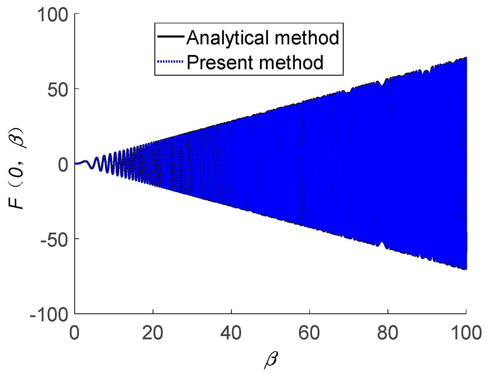
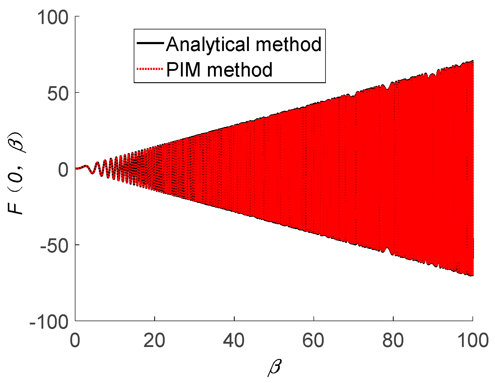
In Figure 3, the “analytical method” denotes the solutions obtained by the analytical expression for TFSGF when $\mu =0$ (presented in Equation (40)). Figure 3 shows the solutions obtained by the “PIM method”, with constant m = 50 for $0\le \beta \le 100$ [27].

Figure 3. The $F\left(0,\beta \right)$ computed by “precise integration method (PIM) method” with $\Delta \beta =0.02$.

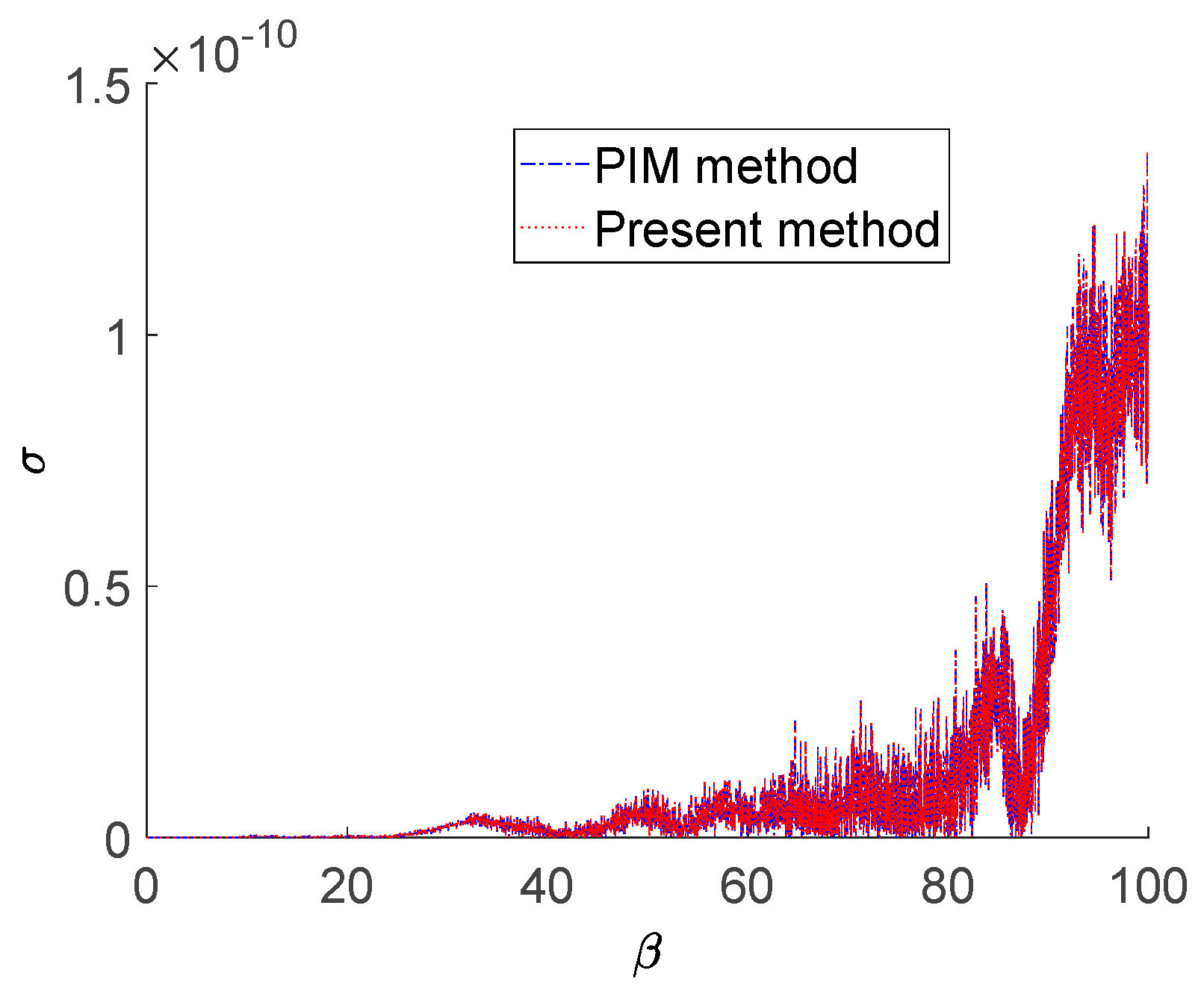
In Figure 4, “present method” denotes solutions of TFSGF solved by PIM method, with variable m for $0\le \beta \le 100$; in the present study, m = 30 for $0\le \beta \le 60$, m = 40 for $60<\beta \le 80$, and m = 50 for $80<\beta \le 100$, respectively.

Figure 4. The $F\left(0,\beta \right)$ computed by “present method” with $\Delta \beta =0.02$.

Figure 5 shows absolute errors computed by “PIM method” and “present method”, with variable m for $0\le \beta \le 100$; in the present study, m = 30 for $0\le \beta \le 60$, m = 40 for $60<\beta \le 80$, and m = 50 for $80<\beta \le 100$, respectively.

Figure 5. The absolute error $\sigma$ computed by “present method” and “PIM method” with $\Delta \beta =0.02$.

In the present study, all computations are carried out on the platform Intel(R) Core (TM) i7700HQ CPU 2.80 GHz. From Figure 3, Figure 4 and Figure 5, the “PIM method” takes about 236.38 s to generate TFSGF at $1\times 5000$ sets of $\left(\mu ,\beta \right)$ for $0\le \beta \le 100$ at $\mu =0$, while the “present method” only takes about 85.8 s. The absolute errors of both “present method” and “PIM method” are within ${10}^{-9}$. Thus, the “present method” shows better evaluation efficiency than the “PIM method”.

4.2. The Study Case and Parameter Setting

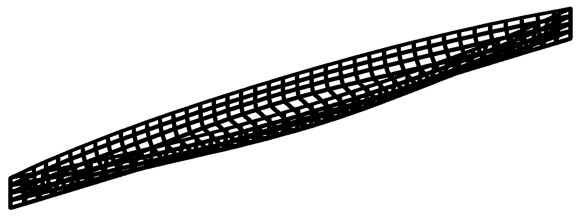
The hull form of Wigley I hull can be defined as in the reference [29]

$$\frac{y}{B/2}=\left[1-{\left(\frac{2x}{L}\right)}^2\right]\left[1-{\left(\frac{z}{D}\right)}^2\right]\left[1+0.2{\left(\frac{2x}{L}\right)}^2\right]+{\left(\frac{z}{D}\right)}^2\left[1-{\left(\frac{z}{D}\right)}^4\right]{\left[1-{\left(\frac{2x}{L}\right)}^2\right]}^4$$

(41)

where $L$ is the length of the ship; $B$ is the width of the ship; $D$ is the draft of the ship.

The main particulars of the Wigley I hull are given in Table 2; $k_{yy}$ denotes the pitch inertia radius of the ship, and $\nabla$ denotes the displacement volume of the ship.

Table 2. Main particulars of the Wigley I hull.

Ship	$\mathit{L}$/m	$\mathit{B}$/m	$\mathit{D}$/m	${\mathit{k}}_{\mathit{y}\mathit{y}}$	∇ $\mathbf{/}{\mathit{m}}^{\mathbf{3}}$
Wigley I hull	3.0	0.3	0.1875	0.25 L	0.0946

The meshes of the ship’s hull are illustrated in Figure 6.

Figure 6. The panels’ distribution on the Wigley I hull.

Non-dimensional forms of hydrodynamic coefficient, memory function, wave exciting forces, and motion response are given below.

The non-dimensional added mass coefficients are defined as $A_{33}^{\prime }=A_{33}/\left(\rho \nabla \right)$ and $A_{55}^{\prime }=A_{55}/\left(\rho \nabla L^2\right)$, respectively.

The non-dimensional damping coefficients are defined as $B_{33}^{\prime }=\sqrt{L/g}{B}_{33}/\left(\rho \nabla \right)$ and $B_{55}^{\prime }=\sqrt{L/g}{B}_{55}/\left(\rho \nabla L^2\right)$, respectively.

The heave memory function $K_{33}^{\prime }$ and pitch memory function $K_{55}^{\prime }$ are defined as $K_{33}^{\prime }=\left(K_{33}L\right)/\left(\rho g\nabla \right)$ and $K_{55}^{\prime }=K_{55}/\left(\rho g\nabla \right)$, respectively.

The non-dimensional wave exciting forces are defined as $F_{3\mathrm{w}}^{\prime }=F_{3\mathrm{w}}L/\left(\rho g{\eta }_0\nabla \right)$ and $F_{5\mathrm{w}}^{\prime }=F_{5\mathrm{w}}/\left(\rho g{\eta }_0\nabla \right)$, respectively.

The non-dimensional heave and pitch motion are defined as ${\zeta }_3^{\prime }={\zeta }_3/{\eta }_0$ and ${\zeta }_5^{\prime }=\left({\zeta }_{5}L\right)/\left(2\mathsf{\pi }{\eta }_0\right)$, respectively.

The non-dimensional frequency ${\omega }^{\prime }$ is defined as ${\omega }^{\prime }=\omega \sqrt{L/g}$, the non-dimensional wave number ${\upsilon }^{\prime }$ is defined as ${\upsilon }^{\prime }=\upsilon L$, and the non-dimensional frequency $t^{\prime }$ is defined as $t^{\prime }=t/T_{\mathrm{e}}$ ($T_{\mathrm{e}}$ is encounter period).

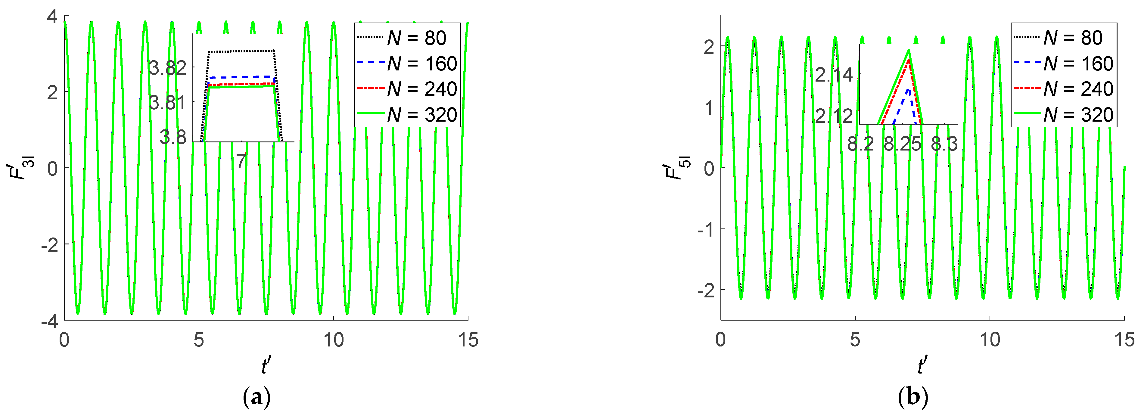
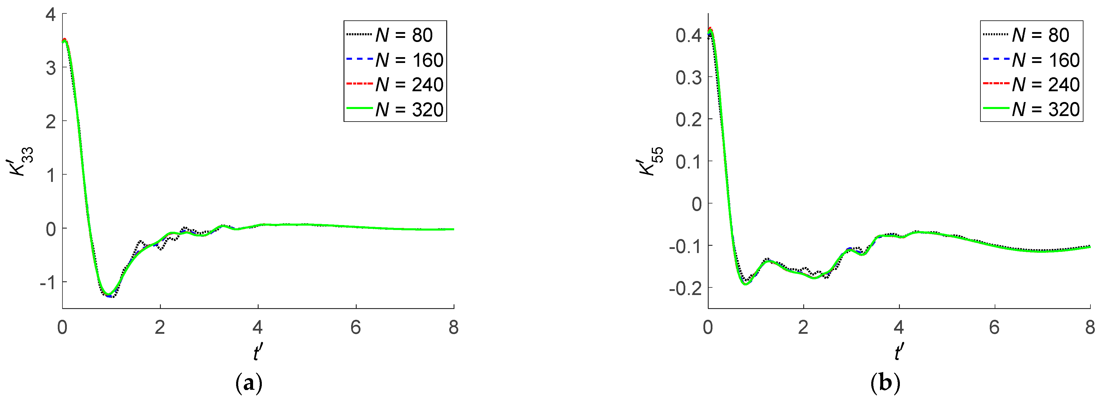
4.3. The Convergence Study on Panel Number N and Time Step $\Delta t$

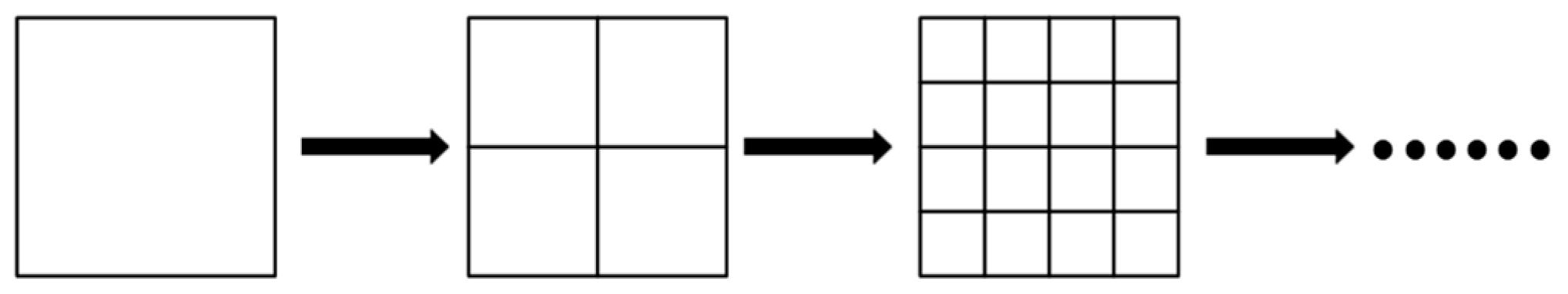
The panel number N and the time step $\Delta t$ have influences on the numerical results of ship hydrodynamic analysis and ship motion. The convergence of the two parameters is verified by taking the Wigley I hull as a study case. The error of 0.1% is adopted to test convergence. Wigley I hull is studied at Fn = 0.2 (Fn denotes Froude number, $Fn=U/\sqrt{gL}$) in head seas ($\alpha =\mathsf{\pi }$, ${\eta }_0=0.036$ m).

The $2\times 2$ Gaussian quadrature [15] can be used to compute the F–K forces and hydrodynamic forces acting on the panel. As shown in Figure 7, the square panel can be progressively subdivided until the prescribed precision is reached.

Figure 7. The panel subdivision diagram.

The four different panel numbers of the Wigley I hull surface discretization with constant time step $\Delta t=T_{\mathrm{e}}/40$ are carried out (Table 3).

Table 3. Panel numbers for the convergence analysis of Wigley I hull discretization.

Case	1	2	3	4
Wigley I	$N=20\times 4$	$N=40\times 4$	$N=60\times 4$	$N=80\times 4$

Figure 8 illustrates the time history of the heave memory function and pitch memory function.

Figure 8. Non-dimensional memory function of Wigley I hull: (a) heave; (b) pitch.

Figure 9 shows the time history of the non-dimensional F–K forces. The Wigley I hull advances in head regular waves at Fn = 0.2, and the wavelength to ship length is $\lambda /L=1$. F–K forces can be obtained by the Gaussian quadrature method.

Figure 9. Non-dimensional F–K forces of Wigley I hull ($\lambda /L=1$: (a) heave; (b) pitch.

As shown in Figure 8 and Figure 9, the numerical results tend to be convergent when $N\ge 240$, and the relative error between $N=240$ and $N=320$ is within 0.1%. Thus, panel number N = 320 is selected for ship hydrodynamic analysis and ship motion in the present study.

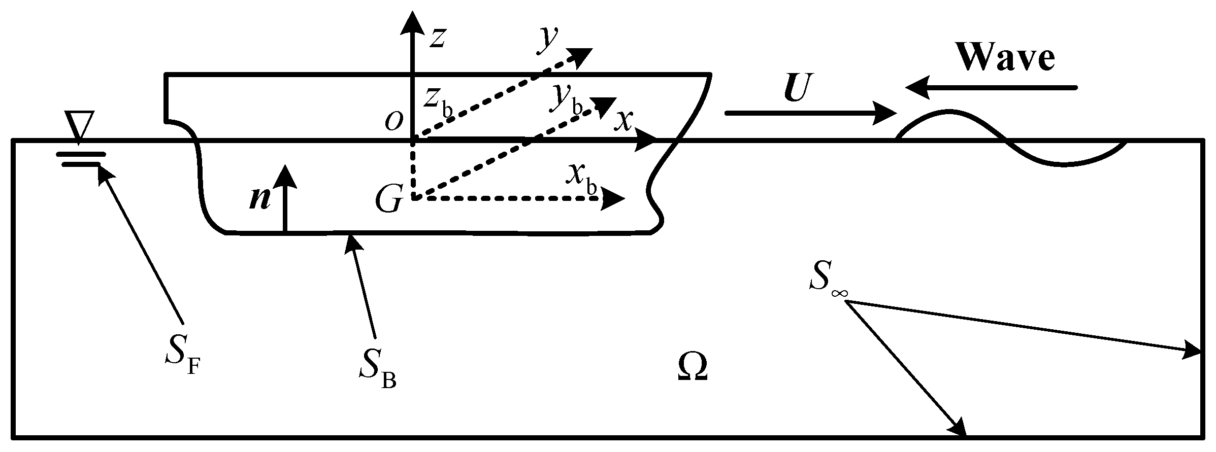
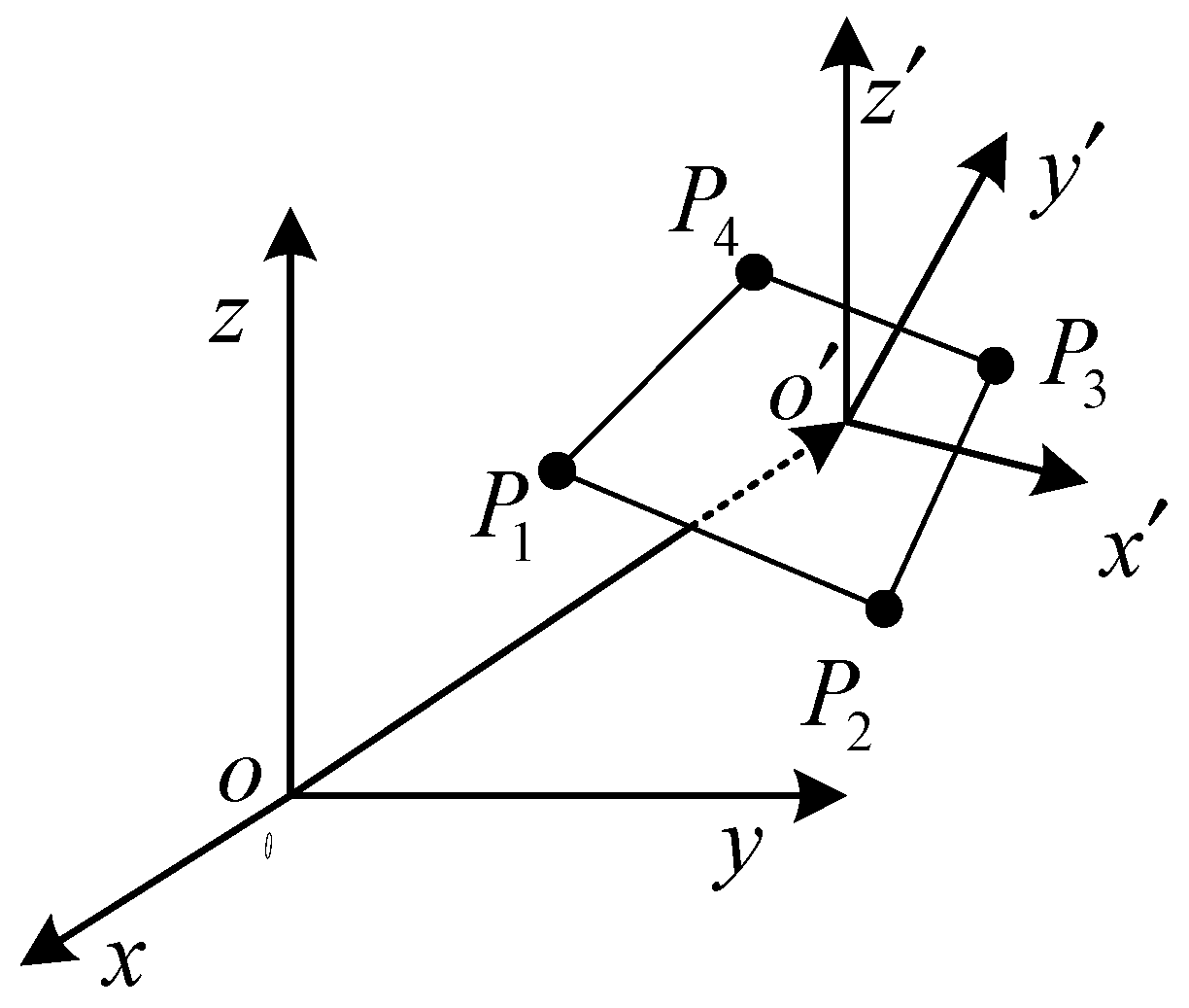
In the system $o\text{-}xyz$, a square panel is adopted as a study case advancing in head regular waves, whose four vertices are $P_1\left(-0.5,0,-1\right)$, $P_2\left(0.5,0,-1\right)$, $P_3\left(0.5,0,0\right)$, and $P_4\left(-0.5,0,0\right)$, respectively. The square panel advances in head regular waves at Fn = 0.2, and the wavelength to ship length is 1.5, and the wave steepness is 0.024.

At t = 0, the F–K force acting on the square panel by the analytical integration method is 179.6193 N (the calculation accuracy can be set to 0.0001 N).

From Table 4, as the subdivision time is 4, the square panel can be subdivided into 256 smaller subpanels, as shown in Figure 7. However, the computational results of the Gauss integration method and the analytical integration method are the same. For simple geometry of the ship’s hull, the magnitude of panel number for hull mesh generation can be as low as O(10), such as barge vessel [16]. The analytical integration method can improve the F–K forces evaluation accuracy with no loss of accuracy.

Table 4. Values of F–K forces acting on the panel at t = 0.

Subdivision Time	0	1	2	3	4
F–K forces (unit: N)	179.3024	179.5996	179.6181	179.6192	179.6193
Non-dimensional F–K forces	15.7080	15.7340	15.7357	15.7358	15.7358

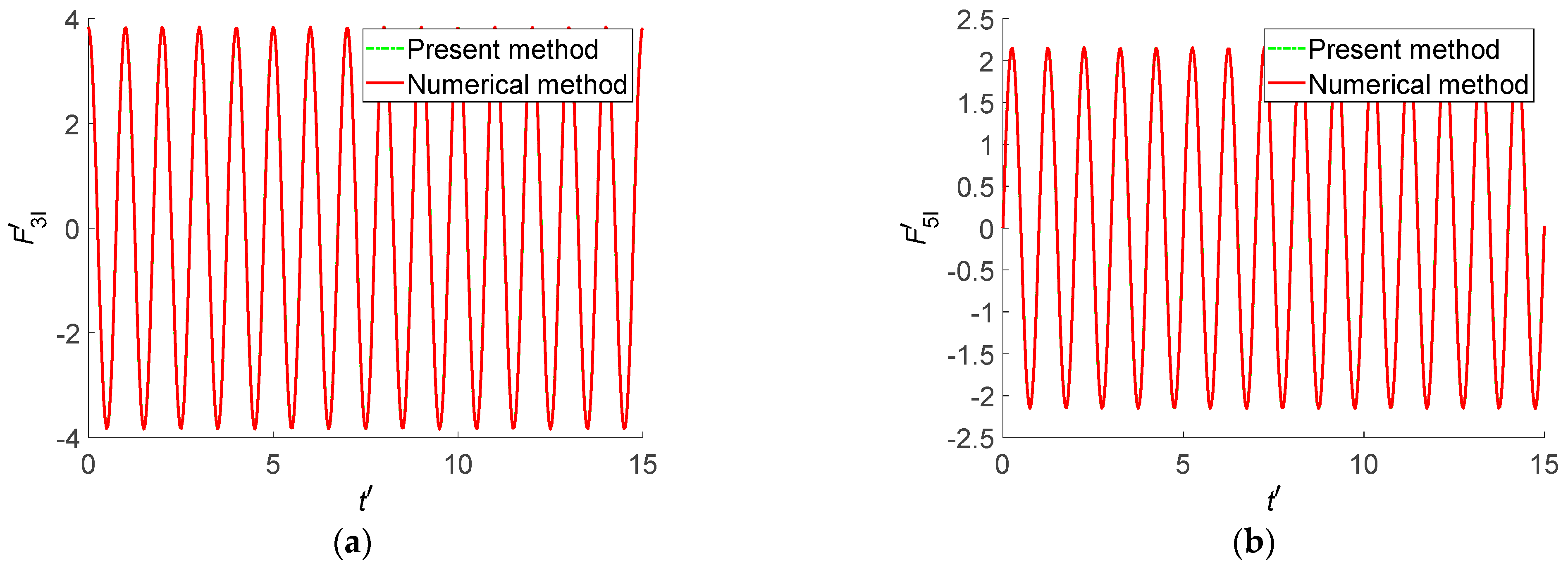
Figure 10 shows the time history of the non-dimensional F–K forces in head regular waves at Fn = 0.2 obtained by “numerical method” and “present method”, respectively. The Wigley I hull surface is discretized and processed into N = 320 quadrilateral panels. “numerical method” denotes the numerical results of F–K forces obtained by $2\times 2$ Gaussian quadrature, and “present method” denotes the results of F–K forces obtained by the analytical method.

Figure 10. Time history of non-dimensional F–K forces of Wigley I hull obtained by “present method” and “numerical method” ($\lambda /L=1$: (a) heave; (b) pitch.

From Figure 10, the F–K forces obtained by “numerical method” and “present method” are almost the same, and the relative error between the “numerical method” and “present method” is 0.1%. The CPU time consumption for the “numerical method” is about 35.4 s, while the CPU time consumption for the “present method” is about 27.8 s. The “present method” is more efficient than the “numerical method”. The efficiency and accuracy of the “present method” can be validated.

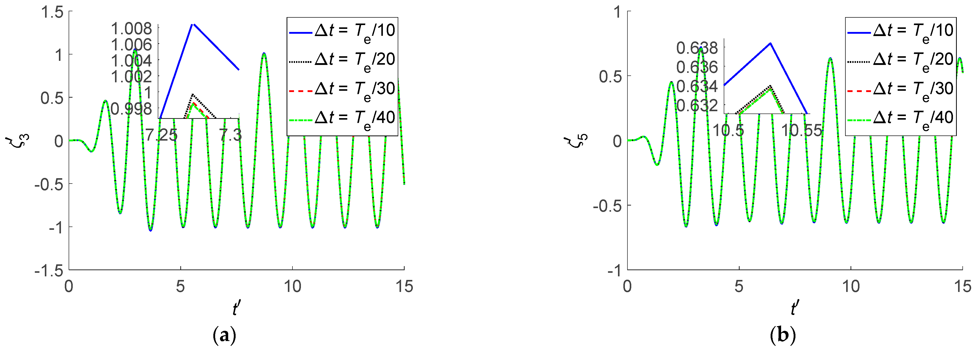
Figure 11 illustrates the time history of heave motion and pitch motion of Wigley I hull with four different time steps, which are $T_{\mathrm{e}}/10$, $T_{\mathrm{e}}/20$, $T_{\mathrm{e}}/30$, and $T_{\mathrm{e}}/40$, respectively.

Figure 11. Time history of motions of Wigley I hull ($\lambda /L=2$, N = 320): (a) heave; (b) pitch.

In Figure 11, as time step $\Delta t$ decreases, a convergent trend can be obtained, and the relative error between $\Delta t=T_{\mathrm{e}}/30$ and $\Delta t=T_{\mathrm{e}}/40$ is within 0.1%. The time step $\Delta t=T_{\mathrm{e}}/40$ is selected for the subsequent ship hydrodynamic analysis and ship motions.

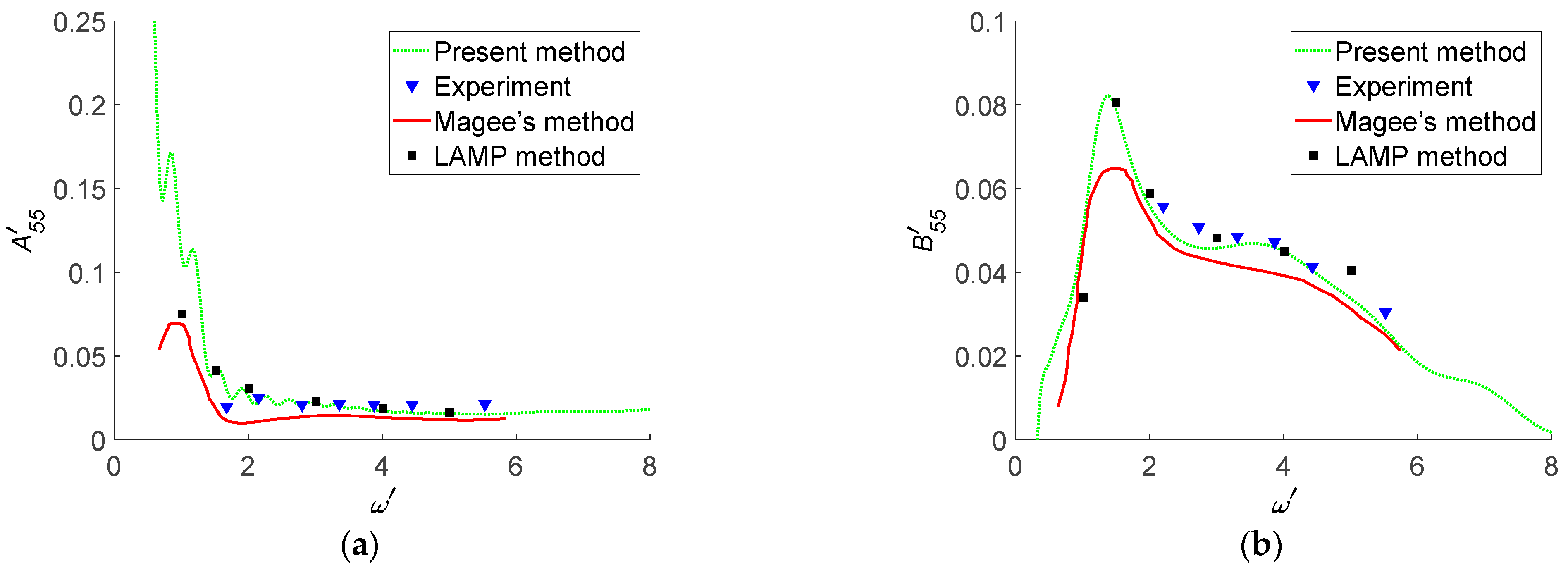
4.4. Added Mass and Damping Coefficient

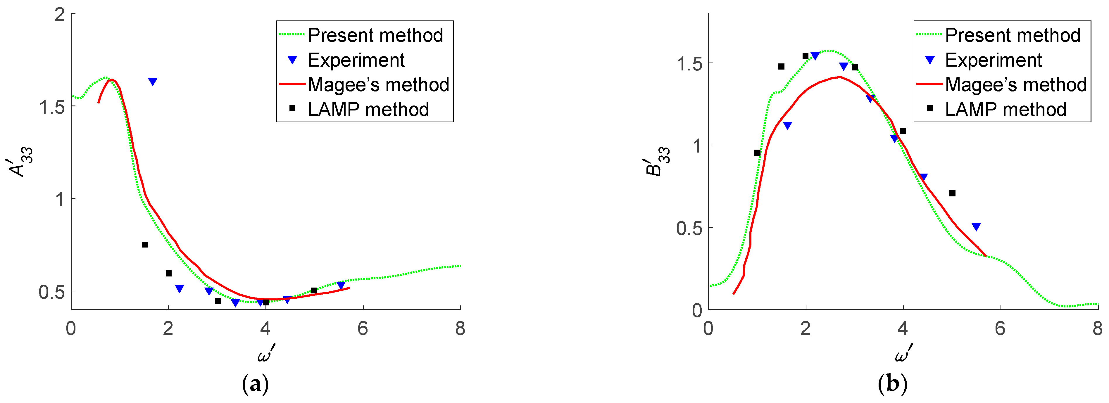
Since the hydrodynamic coefficients on the main diagonal have a significant influence on ship hydrodynamic analysis and motion, the non-dimensional coefficients $A_{33}^{\prime }$, $A_{55}^{\prime }$, $B_{33}^{\prime }$, and $B_{55}^{\prime }$ are selected for detailed numerical analysis.

For the Wigley I hull at Fn = 0.2, Figure 12 presents the comparisons of the non-dimensional heave-heave added masses and damping coefficients, and Figure 13 presents the comparisons of the non-dimensional pitch-pitch added masses and damping coefficients. In the legend of Figure 12 and Figure 13, “present method” denotes numerical results obtained by the TFSGF method without waterline terms in Equation (5). “experiment” denotes previous literature experimental data [29] obtained by Journée, and the experiments were carried out in the Shiphydromechanics Laboratory of the Delft University of Technology. The experimental data on hydrodynamic coefficients, wave loads, and added resistance for heave and pitch motions in head waves of Wigley I hull are sufficient. “Magee’s method” denotes numerical results obtained by the TFSGF method [28] in which the waterline integral terms of boundary integral equations are included. “LAMP method” denotes numerical results obtained by LAMP software [21], in which the body nonlinear method was adopted where the perturbation potential was computed on the instantaneous wetted hull under the mean free surface.

Figure 12. Non-dimensional heave-heave added mass and damping coefficients: (a) $A_{33}^{\prime }$; (b) $B_{33}^{\prime }$.

Figure 13. Non-dimensional pitch-pitch added mass and damping coefficients: (a) $A_{55}^{\prime }$; (b) $B_{55}^{\prime }$.

Table 5, Table 6, Table 7 and Table 8 present absolute relative errors of hydrodynamic coefficients for Wigley I hull by “present method” and “Magee’s method”, which are compared with previous literature experimental data [29]. The absolute relative error can be written as $\epsilon =\left|\left(N_{\mathrm{num}}-N_{\exp }\right)/N_{\exp }\right|$ ($\epsilon$ denotes absolute relative error, $N_{\mathrm{num}}$ denotes numerical results obtained by various models, and $N_{\exp }$ denotes a value for previous literature experimental data [29]).

Table 5. Absolute relative errors of heave-heave added mass $A_{33}$ for Wigley I hull by various methods.

${\mathit{\omega }}^{\mathbf{\prime }}$	2.2	2.8	3.3	3.9	4.4	5.5
Present method	31.7%	3.7%	2.8%	1.4%	0.2%	2.5%
Magee’s method	40.6%	12.2%	11.0%	2.4%	0.2%	5.6%

Table 6. Absolute relative errors of heave-heave damping coefficients $B_{33}$ for Wigley I hull by various methods.

${\mathit{\omega }}^{\mathbf{\prime }}$	2.2	2.8	3.3	3.9	4.4	5.5
Present method	0.1%	3.9%	4.2%	1.9%	10.6%	33.5%
Magee’s method	11.5%	5.1%	1.0%	4.8%	4.2%	23.9%

Table 7. Absolute relative errors of pitch-pitch added mass $A_{55}$ for Wigley I hull by various methods.

${\mathit{\omega }}^{\mathbf{\prime }}$	2.2	2.8	3.3	3.9	4.4	5.5
Present method	9.9%	2.3%	3.3%	17.1%	23.3%	28.5%
Magee’s method	57.0%	34.5%	32.1%	35.0%	40.0%	43.7%

Table 8. Absolute relative errors of pitch-pitch damping coefficients $B_{55}$ for Wigley I hull by various methods.

${\mathit{\omega }}^{\mathbf{\prime }}$	2.2	2.8	3.3	3.9	4.4	5.5
Present method	8.2%	9.7%	4.1%	2.6%	2.1%	14.0%
Magee’s method	14.6%	14.3%	14.7%	16.0%	11.0%	18.07%

From Figure 12 and Figure 13, resonance occurs around the non-dimensional frequency ${\omega }^{\prime }=1.40$, and there is a larger deviation between numerical results and previous literature experimental data [29]. As the non-dimensional frequency increases, hydrodynamic coefficients obtained from “present method”, “Magee’s method”, and “LAMP method” show a similar change trend. From Table 5, Table 6, Table 7 and Table 8, the numerical results obtained by the “present method” are in better agreement with the previous literature experimental data [29] than those obtained by “Magee’s method”. Based on the potential flow assumption, the viscosity of a fluid is ignored. When both the field point and source point are on the mean free surface, the amplitude and oscillating frequency of TFSGF increase rapidly with time parameter $\beta$, and there will be a larger numerical error if waterline integral terms of boundary integral equations are included. The accuracy for hydrodynamic coefficient evaluation can be improved by the present method with waterline integral terms excluded.

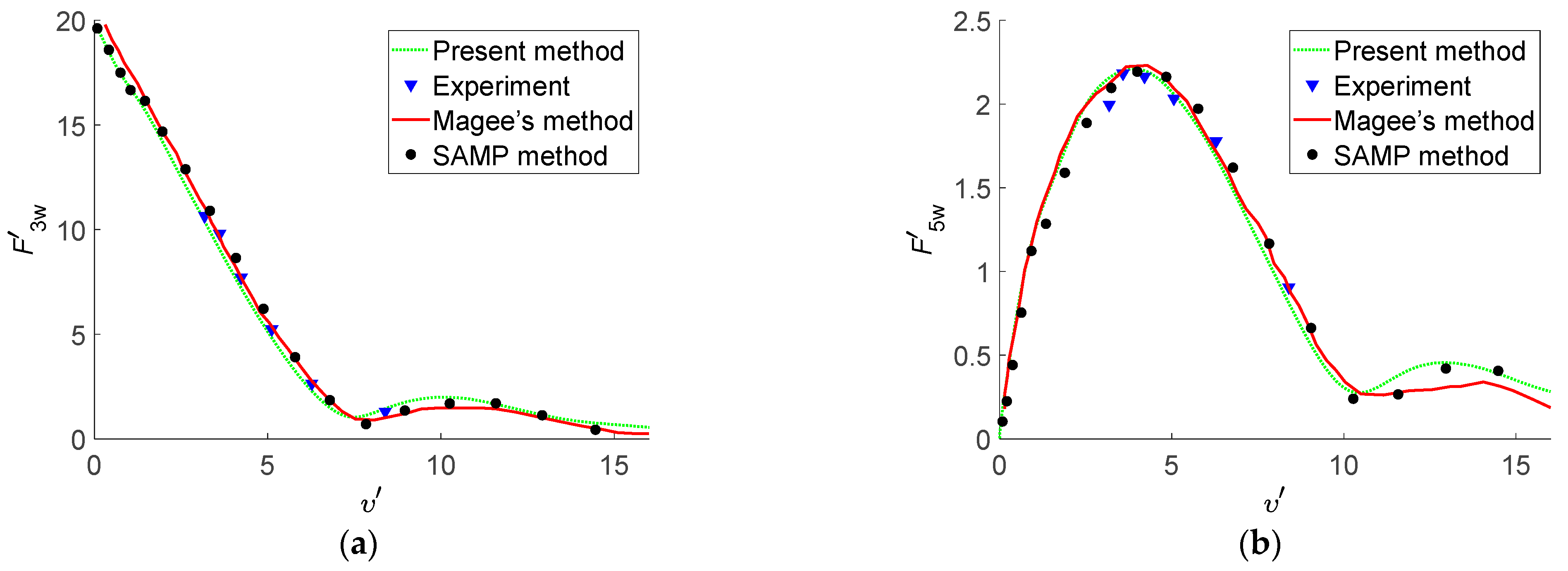
4.5. The Wave Exciting Forces

The Wigley I hull advances in head regular waves at Fn = 0.2. The wave exciting forces are composed of F–K forces and diffraction forces in the frequency domain, and diffraction forces in the frequency domain can be obtained by Fourier transformation [15]. Figure 14 shows the numerical results of amplitudes of the non-dimensional wave exciting forces obtained by various methods. ”SAMP method” denotes numerical results obtained by a transient free surface Green function method in the linear time domain [21].

Figure 14. Non-dimensional wave exciting force amplitude at Fn = 0.2: (a) heave; (b) pitch.

From Figure 14, the maximum relative error between “present method” and “experiment” is within 10.0%, and the non-dimensional wave exciting forces obtained from “present method”, “Magee’s method” and ”SAMP method” show a similar change trend. Thus, the reliability of analytical expression for F–K forces evaluation is verified.

4.6. The Motion Responses

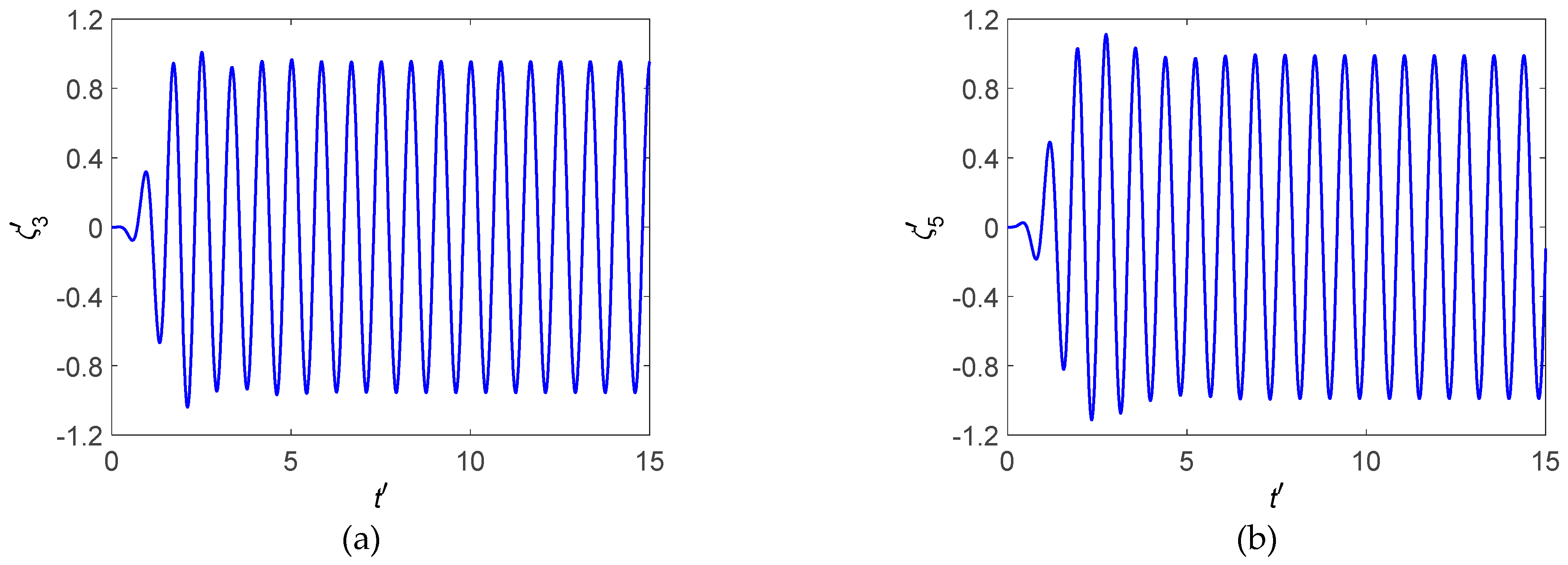
Figure 15 shows the time history of motions of Wigley I hull at Fn = 0.2 in head regular waves ($\alpha =\mathsf{\pi }$).

Figure 15. Non-dimensional time history of motions of Wigley I hull ($\lambda /L=1.5$): (a) heave; (b) pitch.

From Figure 15, the instantaneous influences of the initial disturbance on the time history of motion disappear after about 3~5 wave periods. Thus, the three-dimensional linear time-domain simulation program developed in the present study is numerically stable.

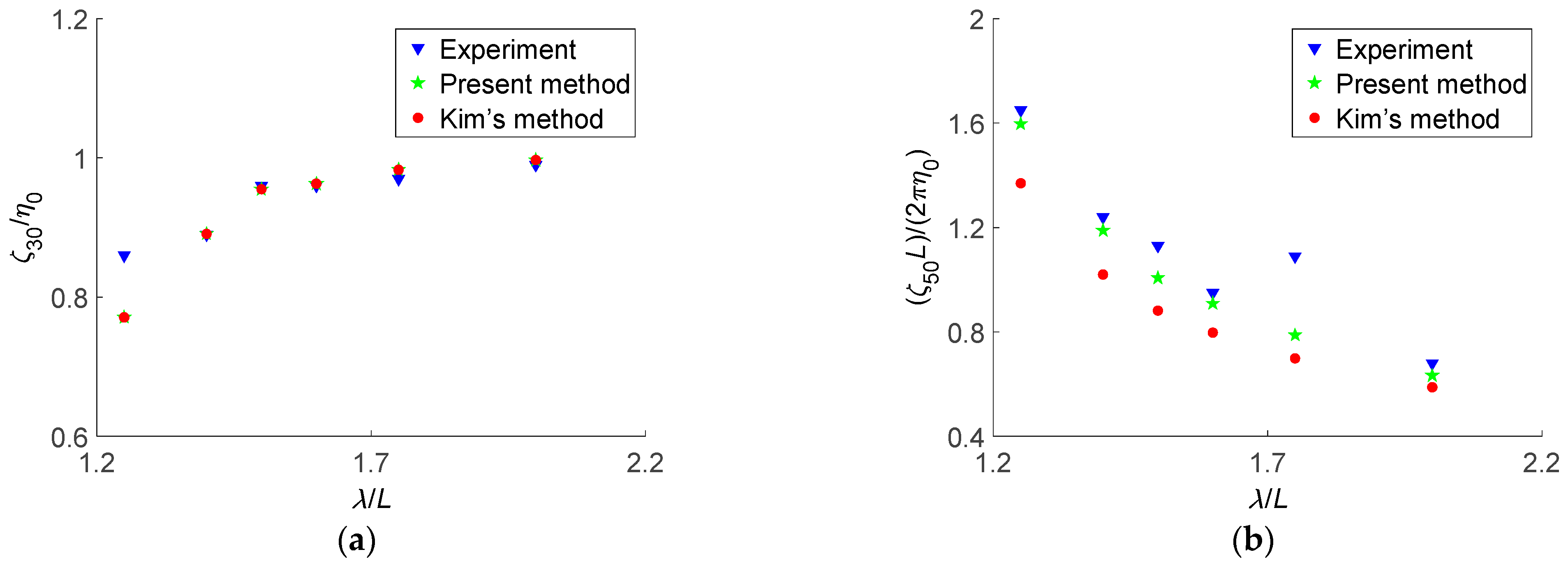
Figure 16 shows heave response amplitude operators (Raos) and pitch response amplitude operators for ship motions in head regular waves at Fn = 0.2. The response amplitude of heave motion can be defined as ${\zeta }_{30}/{\eta }_0$, and ${\zeta }_{30}$ is the amplitude of ship heave motions. The response amplitude of pitch motion can be defined as $\left({\zeta }_{50}L\right)/\left(2\mathsf{\pi }{\eta }_0\right)$, and ${\zeta }_{50}$ is the amplitude of ship pitch motions. In Figure 16, “Kim’s method” denotes the numerical results obtained by a three-dimensional Rankine panel method in the linear time domain [35].

Figure 16. Response amplitude operators of motion for Wigley I hull at Fn = 0.2 in head regular waves: (a) heave; (b) pitch.

From Figure 16, for ship heave motion responses, both “present method” and “Kim’s method” can be in good agreement with previous literature experimental data [29]; for ship pitch motion responses, the numerical results obtained by “present method” are closer to previous literature experimental data [29] than those obtained by “Kim’s method”. When $\lambda /L$ approaches 1.80, the numerical results of the pitch motion responses show non-ignorable errors compared with the previous literature experimental data [29]. As $\lambda /L$ approaches 1.80, the wave encounter frequency is nearly equal to the natural frequency of pitch motion. Thus, the resonance can take place, and the previous literature experimental data [29] is quite larger than the numerical results. In the present study, the TFSGF method is adopted to solve ship motion problems. The TFSGF can automatically satisfy the free surface boundary condition, and the numerical errors involved in radiation boundary conditions can be reduced. Thus, the numerical results obtained by the “present method” can be in better agreement with previous literature experimental data [29] than “Kim’s method”.

5. Conclusions

In the present study, a three-dimensional time-domain panel method is developed to study the ship’s hydrodynamic analysis and motions in regular waves. The Wigley I hull is taken as a study case. The following conclusions can be made based on numerical simulation and investigations:

(1)

The precise integration method with variable parameter m is adopted for TFSGF evaluation, which can improve the efficiency and numerical stability. It can provide a reliable solver for a ship’s hydrodynamic analysis.

(2)

Based on the TFSGF method, the boundary integral equation without waterline terms is established to solve the perturbation velocity potential. When $\mu =0$, the violent oscillation and amplitude amplification characteristics of TFSGF could lead to worse numerical calculation results. The numerical results of hydrodynamic coefficients obtained by the present method can be in good agreement with previous literature experimental data [29]. In comparison with the TFSGF method, including waterline terms, the present method shows higher accuracy.

(3)

The derived analytical integration expressions for F–K forces evaluation over quadrilateral panels have been proved to provide exact results. For a much simple hull shape, like a barge vessel, only about ten quadrilateral panels are required to discretize the hull body, which needs much fewer mesh grids than the Gauss integration method. The wave exciting forces of the Wigley I hull in regular head waves are in good agreement with both previous literature experimental data [29] and numerical results by other published results [21,28]. Thus, the algorithm developed for F–K forces can be validated.

(4)

Since TFSGF can automatically satisfy the free surface condition, the ship pitch motion response results obtained by the present method are in better agreement with previous literature experimental data [29] than the three-dimensional Rankine panel method [35].

(5)

Based on the present research work, different levels of nonlinearity can be considered in future study work. The boundary integral equation can be built on the instantaneous wetted hull surface instead of the mean wetted hull surface, in which the body nonlinearity can be incorporated more fully. Moreover, the second-order drift forces can also be derived from the present boundary value problem formulation, which can be used to study the ship maneuvering problem.