Modeling of Breaching-Generated Turbidity Currents Using Large Eddy Simulation

Abstract

Breaching flow slides result in a turbidity current running over and directly interacting with the eroding, submarine slope surface, thereby promoting further sediment erosion. The investigation and understanding of this current are crucial, as it is the main parameter influencing the failure evolution and fate of sediment during the breaching phenomenon. In contrast to previous numerical studies dealing with this specific type of turbidity currents, we present a 3D numerical model that simulates the flow structure and hydrodynamics of breaching-generated turbidity currents. The turbulent behavior in the model is captured by large eddy simulation (LES). We present a set of numerical simulations that reproduce particular, previously published experimental results. Through these simulations, we show the validity, applicability, and advantage of the proposed numerical model for the investigation of the flow characteristics. The principal characteristics of the turbidity current are reproduced well, apart from the layer thickness. We also propose a breaching erosion model and validate it using the same series of experimental data. Quite good agreement is observed between the experimental data and the computed erosion rates. The numerical results confirm that breaching-generated turbidity currents are self-accelerating and indicate that they evolve in a self-similar manner.

1. Introduction

Turbidity currents are buoyancy-driven underflows generated by the action of gravity on the density difference between a fluid-sediment mixture and the ambient fluid. The excess hydrostatic pressure within the turbidity current drives the current downstream while complicated interactions with the surrounding environment take place; it interacts with the ambient fluid at the upper boundary and with the bed at the lower boundary, producing turbulence at both boundaries [1]. Turbidity currents are vital agents of sediment transport that deliver sediment from the river mouths to deeper waters [2]. Moreover, they pose a serious threat to flood defense structures, such as dikes and embankments [3], and submarine structures placed at the seafloor, such as oil pipelines, and communication cables [4].

Turbidity currents can be triggered through several mechanisms, such as hypopycnal river plumes [5], internal waves or tides [6], and submarine slope failures [7]. One of the complex failure mechanisms of submarine slopes is the flow slide [8], which takes place when a large amount of sediments in an underwater slope is destabilized and consequently runs down the slope as a dense fluid. Two categories are distinguished: liquefaction flow slides, which occur in loosely packed sand, and breaching flow slides, which mostly occur in densely packed sand [9,10]. The former results in slurry-like or hyper-concentrated density flows, while the latter results in turbidity currents [11]. Here, the focus is on the turbidity current accompanying breaching flow slides, referred to as a breaching-generated turbidity current. These currents have proved very difficult to measure in the field, as their occurrence is unpredictable while they can also destroy the measuring instruments [12,13]. Alternatively, laboratory experiments are widely used (e.g., [14,15,16,17]) and can be scaled and conducted under more controlled conditions to develop a better understanding of the behavior of turbidity currents, and to provide measurements for the validation of numerical models.

To this end, Alhaddad et al. [18] have recently conducted large-scale experiments, obtaining direct measurements of breaching-generated turbidity currents and the associated sediment transport. Their analysis showed that breaching-generated turbidity currents are self-accelerating; the current strengthens itself by the accumulated erosion of sediment from the breach face. The results also suggested that the velocity profiles of these currents are self-similar. Analysis of particle concentration profiles showed that the concentration decays exponentially from the breach face until the upper boundary of the current. Near-bed concentrations were found to be high, reaching 0.4 by volume or even higher in some cases. Moreover, investigation of the slope failure indicated that its evolution is largely three-dimensional. Sand erosion rates in the middle of the tank width, where turbidity currents were measured, were found to be higher than at the tank glass wall, where the erosion rates were measured. A key finding was that the turbidity current is the main parameter controlling the evolution of the breaching failure and the fate of eroded sediment. This implies that a thorough understanding of the behavior of this current is needed to enhance the knowledge about breaching. Owing to the several difficulties associated with breaching experiments, measurements of turbulence quantities of the flow were not possible. The absence of such measurements hinders the estimate of the flow-induced bed shear stress and hence the predication of erosion during breaching. This highlights the need for using advanced numerical models as a complementary tool to the experimental work, to gain new insights into the behavior and structure of breaching-generated turbidity currents.

Many numerical models for density or gravity currents have been proposed in the literature (e.g., [19,20,21,22,23]). To date, however, there are very few numerical investigations dealing with breaching-generated turbidity currents [3,11,24]. Moreover, these numerical efforts were mostly restricted to layer-averaged, one-dimensional models. The model of [24] was applied to simulate a flushing event in Scripps Submarine Canyon, and showed that breaching-generated turbidity currents can excavate a submarine canyon. Similarly, the model of [11] was applied to a flushing event in Monterey submarine canyon. These depth-averaged models require several empirical closure relations (e.g., the near-bed concentration, bed shear stress, and water entrainment at the upper boundary), which reduces the accuracy of the simulation results [25]. Alhaddad et al. [3] applied the one-dimensional model of [26] to a typical case of a breaching slope, demonstrating that the results are highly sensitive to the type of breaching closure relation used.

To reduce these uncertainties, this study presents large eddy simulations of breaching-generated turbidity currents. Large eddy simulations have the advantage that the larger turbulent scales—containing the bulk of the turbulent kinetic energy—are resolved. In this manner, the influence of density gradients on turbulence production is captured adequately, while including the non-isotropic character of turbulence. Therefore, large eddy simulations can provide a wealth of insights into the structure and physical behavior of turbidity currents, in particular into the turbulence structure including turbulent kinetic energy and Reynolds stresses. The numerical model that we use has been applied earlier to gain insights into the complicated dredge plume behavior close to a dredging vessel where density differences, turbulent mixing and sediment settling play an important role [27,28,29]. The model has been validated for a wide range of flow cases relevant to the present study, such as the front speed of density currents radially spreading and density currents running over both flat and sloping beds, the deposition from high-concentration suspended sediment flow at a flat bed [30], and high sediment concentration conditions encountered in hopper sedimentation [31]. In this paper, the implementation is designed to capture the turbidity current running down the slope surface (or ‘breach face’), considering various steep slope inclinations, which were tested in the laboratory experiments. The triggering mechanism of turbidity currents in this work is different from the standard lock-exchange configuration mostly used in the numerical models; sediment particles are released from the bed surface, generating the flow. An adequate prediction of this process has been always difficult, as it involves both geotechnical and hydraulic features [3]. To date, furthermore, no validation of existing breaching erosion models has been presented.

The paper proceeds as follows. We first provide some background of the numerical model in Section 2, and propose a breaching erosion closure model in Section 3. Section 4 revisits the experimental measurements of [18], and validates the performance and limitations of the currently proposed numerical model in characterizing the breaching-generated turbidity currents based on the experimental findings. Following that, Section 5 discusses the flow and turbulence structure and analyses the sensitivity of the numerical results to some initial conditions.

2. Numerical Model Description

2.1. Governing Equations

The flow of water-sediment mixtures—as in breaching-generated turbidity currents—is mathematically described by the incompressible, variable density Navier–Stokes equations. Using the mixture approach, the concentrations of the individual sediment fractions are solved separately while one set of momentum equations is solved for the water-sediment mixture [32]. Each sediment fraction has its own drift velocity ${\mathit{u}}_d$, defined as the velocity of the sediment relative to the water-sediment mixture, which involves a correction of the mixture velocity with the settling velocity of the sediment including the influence of hindered settling. Furthermore, the sediment concentration influences the mixture density. The mixture approach combined with the drift velocity is thus two-way coupling and has proved valid to simulate high-concentration suspended sediment flows (e.g., [31,33,34,35]).

To this end, the corresponding balance equations for the total mass and momentum of the mixture are stated as, respectively,

$$\frac{\partial \rho }{\partial t}+\nabla ·\left(\rho \mathit{u}\right)=0,$$

(1)

$$\frac{\partial \rho \mathit{u}}{\partial t}+\nabla ·(\rho \mathit{u}\otimes \mathit{u})=-\nabla P+\nabla ·\mathit{\tau }+(\rho -{\rho }_w)\mathit{g},$$

(2)

where t denotes time, $\rho$ is the mixture density, ${\rho }_w$ is the water density, $\mathit{u}$ is the mixture velocity vector, P is the modified pressure, $\mathit{\tau }$ is the shear stress tensor, $\mathit{g}$ is the gravity vector, and ∇ denotes the spatial gradient operator. The mixtures that we consider are primarily Newtonian in rheology [36] for which the shear stress tensor is proportional to the deviatoric strain rate of the mixture velocity, as follows,

$$\mathit{\tau }=2\mu \left({\nabla }^s\mathit{u}-\frac{1}{3}\nabla ·\mathit{u}\right),$$

(3)

where $\mu$ is the dynamic viscosity of the mixture and ${\nabla }^s\left(·\right)=\frac{1}{2}\nabla \left(·\right)+\frac{1}{2}\nabla {\left(·\right)}^T$ is the symmetric gradient operator. It is to be noted that Equation (3) is valid only if the layer-averaged volumetric sediment concentration is below the Bagnold limit of ca. 9% beyond which the particle-particle interactions will render the mixture non-Newtonian [37]. In our case, observed layer-averaged concentrations are generally below 9% (see Section 6.1), while in the center and outer region of the turbidity current, concentrations are even smaller due to the entrainment of ambient fluid and the subsequent turbulence mixing [38]. This motivates the use of Equation (3), although in the inner region near the bed the relatively high concentration may require the reconsideration of additional effects on the rheology of the fluid in the boundary layer, leaving room for improvement of our model (see also the discussion in Section 5.3).

Although the mixture model admits multiple sediment fractions [30], a single sediment fraction suffices here, as uniform sediment will be considered. In this case the mixture density is given by,

$$\rho ={\rho }_w+({\rho }_s-{\rho }_w)c,$$

(4)

where ${\rho }_s$ is the density of sediment, and c is the volumetric sediment concentration. The latter satisfies the following transport equation,

$$\frac{\partial c}{\partial t}+\nabla ·\left({\mathit{u}}_{s}c\right)=\nabla ·(\mathsf{\Gamma }\nabla c),$$

(5)

in which ${\mathit{u}}_s=\mathit{u}+{\mathit{u}}_d$ is the velocity of the sediment fraction, and $\mathsf{\Gamma }$ is the diffusivity which is related to the viscosity $\mu$ by,

$$\mathsf{\Gamma }=\frac{\mu }{{\rho }_{w}Sc},$$

(6)

where $Sc$ is the Schmidt number. Following [30,33], $Sc=0.7$ is adopted in this study and, based on sensitivity analysis, LES results are insensitive to the value of Schmidt number when $Sc$ is close to 1. The drift velocity ${\mathit{u}}_d$ accounts for the effects of hindered settling [39] and the return flow created by the settling particles [30].

For a well-posed problem, Equations (1), (2) and (5) must be supplemented with boundary conditions, while for time dependent problems also initial conditions for the sediment concentration and mixture velocity must be prescribed. Importantly, the interaction of the mixture flow with a sediment bed involves the bed shear stress ${\mathit{\tau }}_b$, and the densimetric sedimentation flux S and erosion flux E given by,

$$S={\rho }_s{c}_b{w}_{s}cos\alpha ,$$

(7)

$$E={\varphi }_{p,t}{\rho }_s\sqrt{\Delta g{d}_{50}},$$

(8)

where $c_b$ is a representative near-bed sediment concentration, $w_s$ is the particle settling velocity, $\alpha$ is the bed slope, $\Delta =({\rho }_s-{\rho }_w)/{\rho }_w$ is the relative submerged sediment density, $d_{50}$ is the median sediment grain size, and ${\varphi }_{p,t}$ is a non-dimensional, so-called, pick-up function involving an empirical closure relation. Given the strong feedback between bed erosion and the hydrodynamics of the turbidity current, the formulation of the pick-up function requires special care to accurately predict the temporal evolution of the slope failure. Section 3.3 will further elaborate on the available theoretical background of sediment erosion during breaching, resulting in the proposed erosion closure model.

2.2. Turbulence Modeling

In our implementation, Equations (1), (2) and (5) are discretized using a regular rectangular grid with, possibly non-uniform, grid sizes ($\Delta x$, $\Delta y$, $\Delta z$ in the respective Cartesian directions). Depending on the grid size, the finite resolution of the computed flow field can only partly include the relevant turbulence length scales. To account for the effect of the unresolved scales on the resolved flow field a turbulence closure model must be used.

In this study, Large Eddy Simulation (LES) is adopted to capture the influence of turbulence. LES applies a spatial filter in which all fluctuations smaller than the grid size are replaced by a sub-grid-scale contribution. In this way, turbulence length scales larger than the grid size are resolved, and the smaller isotropic turbulence scales are accounted for by the sub-grid-scale model. By choosing the grid size sufficiently small, the major part of the turbulent kinetic energy is resolved on the grid and only a small part is modeled by the sub-grid-scale model. An advantage of LES over Reynolds-averaged Navier–Stokes modeling (RANS) is that turbulence damping or destruction functions at sharp density gradients are not needed when sufficient grid resolution is used. This is because the influence of density gradients on the resolved turbulent eddies is automatically taken into account in LES. Furthermore, the non-isotropic behavior of the larger turbulence length scales is resolved in LES. Noteworthy to mention in this respect is that the behavior of the inner region of the turbidity currents, as observed in the experiments, is highly affected by both damping and anisotropy of the turbulence motion in this region.

Following the LES approach, the molecular viscosity ${\mu }_{\mathrm{mol}}$ is enhanced with an extra sub-grid-scale viscosity ${\mu }_{\mathrm{sgs}}$, as follows,

$$\mu ={\mu }_{\mathrm{mol}}+{\mu }_{\mathrm{sgs}},$$

(9)

where ${\mu }_{\mathrm{sgs}}$ is a function of the strain rate tensor and the grid size,

$${\mu }_{\mathrm{sgs}}=\rho {\left(C_S{\left(\Delta x\Delta y\Delta z\right)}^{1/3}\right)}^2∥S∥,$$

(10)

in which $C_S$ is the dimensionless Smagorinsky constant, and $∥S∥$ is the norm of the (filtered) velocity gradient tensor. For the latter, the WALE (wall adapting eddy viscosity) sub-grid-scale turbulence model is adopted together with a constant $C_S$ of 0.325. For details of this implementation see [40].

Turbulence is partly generated at the sediment bed, requiring a formulation of the corresponding boundary conditions consistent with the LES approach. First, the bed shear stress is formulated as a partial slip boundary condition by calculating the local shear velocity $u_{*}$. This is accomplished by assuming a standard logarithmic velocity profile over the grid cell adjacent to the bed, which gives,

$$u_{*}=\frac{{\mathit{u}}_t}{{\kappa }^{-1}ln\left(\frac{1}{2}\Delta Z/Z_0\right)},$$

(11)

where ${\mathit{u}}_t$ is the (filtered) tangential velocity vector in the grid cell adjacent to the bed, $\kappa$ is the Von Kármán constant, $\Delta Z$ is the cell size normal to the bed, and $Z_0=0.11\nu /\left|u_{*}\right|+k_n/30$, in which $\nu$ is the kinematic molecular viscosity of water, and $k_n$ is the Nikuradse roughness height which is set to a value of $2d_{50}$. Next, the bed shear stress, ${\mathit{\tau }}_b$, is computed from,

$${\mathit{\tau }}_b=\rho \left|u_{*}\right|u_{*}.$$

(12)

The corresponding magnitude of the shear velocity, $u_{*}$, is also used in the formulation of the sediment erosion flux E at the bed, which is treated extensively in Section 3.

2.3. Numerical Solution Procedure

The spatial discretization of the model equations is based on the finite volume method, using a rectangular staggered grid in which the discrete velocity and pressure variables are located at alternating points [41]. The discretization in time conforms to a pressure-correction algorithm which involves a predictor step, in which an intermediate velocity field is computed using the pressure from the previous time step, followed by a corrector step, where the velocity and pressure are updated in a coupled fashion in order to satisfy the continuity constraint, Equation (1).

In the predictor step an explicit third order Adams–Bashfort time integration scheme is employed, adjusted to be able to apply variable time step sizes. Small time steps are to be used with the Courant–Friedrichs–Lewy number (CFL-number) staying below $0.6$. The spatial discretization of the convection terms in the momentum equations is crucial for LES and is performed by a stable scheme with very low diffusion [42]. Likewise, the advection term in the transport equation is discretized with an accurate and robust TVD (Total Variation Diminishing) scheme employing the Van Leer limiter.

In the corrector step, the enforcement of the continuity constraint results in a pressure Poisson equation which is solved by a fast direct solver using the methodology of [43]. Although for incompressible single-phase flows the continuity constraint implies zero divergence of the velocity field (by setting $D\rho /Dt=0$ in Equation (1)), this is generally not so for the flow of incompressible mixtures [44]. This owes to the definition of the mixture velocity $\mathit{u}$ in a densimetric manner, while zero divergence only holds for the volumetric mixture velocity. The latter is obtained by correcting the densimetric mixture velocity $\mathit{u}$ with the respective equilibrium settling velocities from all sediment fractions—a necessary step preceding the enforcement of the zero divergence constraint.

Overall, the numerical method is second-order accurate in time and space. For more details on the numerics, the reader is referred to [30].

3. Breaching Erosion Modeling

Breaching can be defined as a gradual, slow, retrogressive erosion of a steep immersed slope, which is steeper than the internal friction angle of the granular material forming that slope. As noted earlier, breaching is largely encountered in densely packed sand, as it exhibits a dilative behavior, when it is subjected to shear forces [9,45]. Dilatancy refers to the expansion of pore volume of sand under shear deformation, which results in the build-up of a negative pore pressure, with reference to the hydrostatic pressure. This negative pressure holds sand particles together and increases the effective stress [46]. An inward hydraulic gradient is developed, as a result of the pressure difference, compelling the neighboring water to flow into the sand pores, and thus releasing the negative pressure. Consequently, sand particles located at the top of the slope surface (breach face) are exclusively undermined and slowly (∼mm/s) peel off, predominantly one by one [3].

The falling sand particles mix with the ambient water, producing a turbidity current running along and interacting with the breach face, and then flowing down the slope toe. This causes an additional shear stress along the breach face, and hence higher erosion. In the conventional sediment pick-up functions, it is assumed that it is impossible for a grain-by-grain sediment erosion to take place in a submerged slope steeper than the internal friction angle. Rather, the erosion may occur as a sudden collapse of the sand body. Nevertheless, breaching refutes this hypothesis [18,47], showing the need for an erosion model compatible with breaching conditions.

It is to be noted that beside the grain-by-grain erosion, an intermittent collapse of coherent sand wedges, termed a surficial slide, was observed in breaching experiments (e.g., [18,47]). The current understanding of these slides remains very limited. In this paper, therefore, we will consider measurements where surficial slides did not take place. This implies that the total erosion will be a combination of particle-by-particle erosion induced by gravity (pure breaching) and sediment erosion induced by the flow motion. In the following, breaching erosion is decomposed into these two main components.

3.1. Pure Breaching

The Dutch industry was the first to explore breaching in the 1970s, and used it as an efficient production mechanism for stationary suction dredgers. In that period, breaching was not known as a failure mechanism of underwater slopes outside the dredging field. To estimate the dredging production, Breusers [48] developed a formula for pure breaching: particle-by-particle erosion induced by gravity. The original formula was derived for a vertical breach face; however, it can be adapted to a general form representing the erosion velocity perpendicular to the breach face for variable inclinations [3]:

$$v_{e,g}=-\frac{sin(\varphi -\alpha )}{sin\varphi }\frac{(1-n_0)}{\delta n}{k}_l\frac{{\rho }_s-{\rho }_w}{{\rho }_w},$$

(13)

where $v_{e,g}$ [$\mathrm{m}/\mathrm{s}$] is the erosion rate of pure breaching, $\varphi$ [${}^{\circ }$] is the internal friction angle, $n_0$ [-] is the in situ porosity of the sand, $k_l$ [$\mathrm{m}/\mathrm{s}$] is the sand permeability at the loose state, ${\rho }_w$ [$\mathrm{kg}/\mathrm{m}$${}^3$] is the density of water, and $\delta n=(n_l-n_0)/(1-n_l)$ is the relative change in porosity, in which $n_l$ [-] is the maximum porosity of the sand.

Pure breaching is particularly sensitive to the magnitude of sand permeability $k_l$ with a linearly proportional relation. This implies that the existence of finer particles within the sand considerably decreases pure breaching, since they fill pore spaces and reduce permeability. Furthermore, the permeability plays a role in the fluid-induced erosion, as it will be shown in the next subsection. Fortunately, the value of the permeability reported in [18] was measured in the lab, partly leading to a proper validation of the current erosion model.

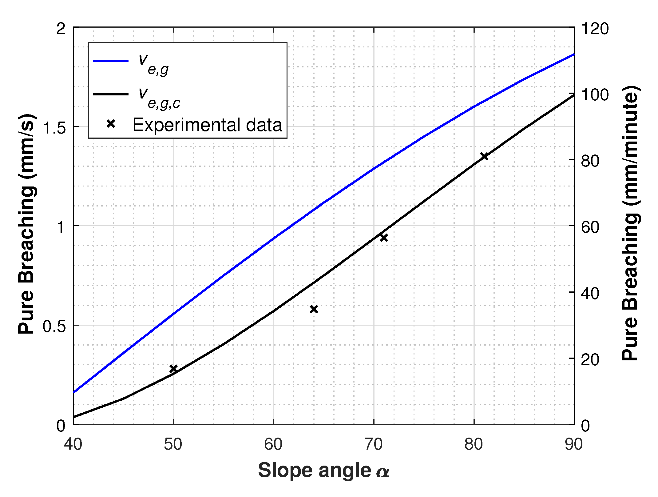
Alhaddad et al. [18] showed that Equation (13) somewhat overestimates pure breaching. Therefore, we propose here an empirical correction factor of $sin{(\alpha -\varphi )}^{0.55}$, which leads to the expression of the corrected pure breaching $v_{e,g,c}$:

$$v_{e,g,c}=-\frac{sin(\varphi -\alpha )sin{(\alpha -\varphi )}^{0.55}}{sin\varphi }\frac{(1-n_0)}{\delta n}{k}_l\frac{{\rho }_s-{\rho }_w}{{\rho }_w}.$$

(14)

Direct measurements of different grain sizes are needed to test the general applicability of this correction factor. Figure 1 depicts the performance of the original and corrected expression of pure breaching. Equation (14) will be used in numerical runs for which no measured pure breaching is available.

3.2. Flow-Induced Erosion

Many parameters play a role in sand erosion induced by turbidity currents, such as near-bed velocity gradient, flow turbulent energy, the properties of sand grains and the bulk properties of sand. In breaching, this part of erosion is more complicated than pure breaching, owing to the special conditions of the breaching process including dilatancy-retarded erosion and a very steep bed [3]. On the one hand, some pick-up functions are proposed in the literature to account for the dilative behavior (e.g., [49]). However, these functions do not account for a sloping bed. On the other hand, some pick-up functions account for the sloping bed (e.g., [50]), but not for a slope steeper than the internal friction angle.

The literature shows, to the best of our knowledge, that only two erosion models were suggested to suit the conditions of the breaching problem [24,45]. These two erosion models are an extension of the formula of [48], meaning that they combine both the pure breaching and sediment erosion by the turbidity current. However, the lack of quantitative data on breaching flow slides has resulted in there being no validation of these erosion models under breaching conditions. Moreover, [3] showed that the erosion rate predicted under the same conditions varies considerably between these erosion models.

3.3. Total Erosion

In this work, we adopt the erosion model of [24] as a basal point and develop it further to improve its predictive ability of breaching erosion. Their erosion model reads

$$\frac{v_{e,t}}{u_{ss}}\left(1-\frac{v_{e,t}}{v_{e,g}}\right)=\frac{{\varphi }_{p,f}}{\frac{sin(\varphi -\alpha )}{sin\varphi }(1-n_0)},$$

(15)

where $v_{e,t}$ is the total erosion velocity including pure breaching and flow-induced erosion, $u_{ss}=\sqrt{\Delta g{D}_{50}}$ is Shields velocity for sand grains, and ${\varphi }_{p,f}$ is an empirical non-dimensional pick-up function, which does not account for the bed dilative behavior nor the sloping bed:

$${\varphi }_{p,f}=\frac{E}{{\rho }_s{u}_{ss}},$$

(16)

where $E={\rho }_s{v}_{e,f}(1-n_0)$ [$\mathrm{kg}/(\mathrm{sm}$${}^2$)] is the sediment pick-up rate perpendicular to the bed surface in which $v_{e,f}$ is the velocity of fluid-induced erosion. The general solution of Equation (15) was not reported in [24]. Instead, two solutions for the two extreme cases $v_{e,t}/v_{e,g}<<1$ and $v_{e,t}/v_{e,g}>>1$ were provided. The first extreme case is never encountered in breaching, while the second extreme case does not hold under lab conditions. Alternatively, Equation (15) can be rearranged into a quadratic equation, and after substituting Equation (13) into the resulting quadratic equation, the general solution will read:

$$v_{e,t}=u_{ss}\left(\frac{v_{e,g}}{2u_{ss}}+\sqrt{\left(\frac{v_{e,g}}{2u_{ss}}\right)+\frac{{\varphi }_{p,f}\Delta k_{l}f}{u_{ss}\delta n}}\right),$$

(17)

where f = 1 if Equation (13) is used for pure breaching, whereas $f=v_{e,g,used}/v_{e,g}$ when another value of $v_{e,g,used}$ is used for pure breaching.

An important feature of breaching-generated turbidity currents is their high particle concentration, the effect of which should be accounted for in the breaching erosion model. High near-bed concentrations reduce the flow-induced sediment erosion [49,51]. The effect of near-bed concentration can be explained by the continuity principle. The sediments are entrained into the flow by the turbulent eddies, and when a turbulent eddy picks up a volume of sediment-water mixture from the bed, the same volume of near-bed mixture has to be conveyed back to the bed. If the near-bed concentration is low, the backflow will carry few sediment particles back to the bed. However, if the near-bed concentration is high, the backflow will carry more sediment particles back to the bed. When the near-bed concentration is almost equal to the bed concentration, nearly no net sediment erosion will take place. Following this argument, [51] put forward the reduction factor $R=(1-n_0-c_b)/(1-n_0)$ to account for the effect of the near-bed concentration $c_b$. Nevertheless, there is no clear definition of the reference line for the near-bed concentration.

To close Equation (17), we propose a new pick-up function ${\varphi }_{p,f}$, which is modified from the existing function of [52]:

$${\varphi }_{p,f}=0.00052R{D}_{*}^{0.3}{\left(\frac{\theta -f_{cr}{\theta }_{cr}}{f_{cr}{\theta }_{cr}}\right)}^{1.5},$$

(18)

where $D_{*}$ is a dimensionless particle diameter defined by $D_{*}=D_{50}\sqrt[3]{\Delta g/\nu }$, in which $\nu$ (m${}^2$/s) is the kinematic viscosity of water, $\theta$ is the Shields parameter, ${\theta }_{cr}$ is the critical Shields parameter for sediment motion and $f_{cr}=1+sin{(\alpha -\varphi )}^2$ is an amplification factor for the critical Shields parameter, which can be used when $\alpha >\varphi$. Lamb et al. [53] demonstrated that there is a clear dependency between the critical Shields stress for sediment motion and the bed slope; the critical Shields stress increases with bed slope. Therefore, we account for this increase by the empirical factor $f_{cr}$.

Here, we assume that the near-bed concentration is the average value of the particle concentrations within the inner region, where the velocity gradient is positive. The reason behind this choice is to reduce the dependency of the value of the near-bed concentration on the mesh resolution, as higher resolution results in higher concentration of the first cell above the bed. We also show the influence of using the concentration of the first cell above the bed as $c_b$ (instead of the average of the inner region) on the erosional characteristics of the flow (see Section 5.2).

In the current numerical tool, the computations are done using a non-dimensional pick-up function rather than an erosion velocity. Therefore, Equation (17) is recast into the total non-dimensional pick-up function, which reads

$${\varphi }_{p,t}=\frac{v_{e,t}(1-n_0)}{u_{ss}}.$$

(19)

It is worth noting that [24] did not account for sediment deposition in their formula, as it was assumed that sedimentation is negligible compared to erosion. However, this assumption may be valid for low near-bed concentrations. In breaching, the near-bed concentrations can be very large. In the model, therefore, we include the sedimentation flux (Equation (7)), leading to a reduction of the erosion velocity equal to the sedimentation velocity $v_s=(c_b{w}_{s}cos\alpha )/(1-n_0)$. This means that the erosion velocities resulting from the simulations are the net magnitudes.

4. Model Application

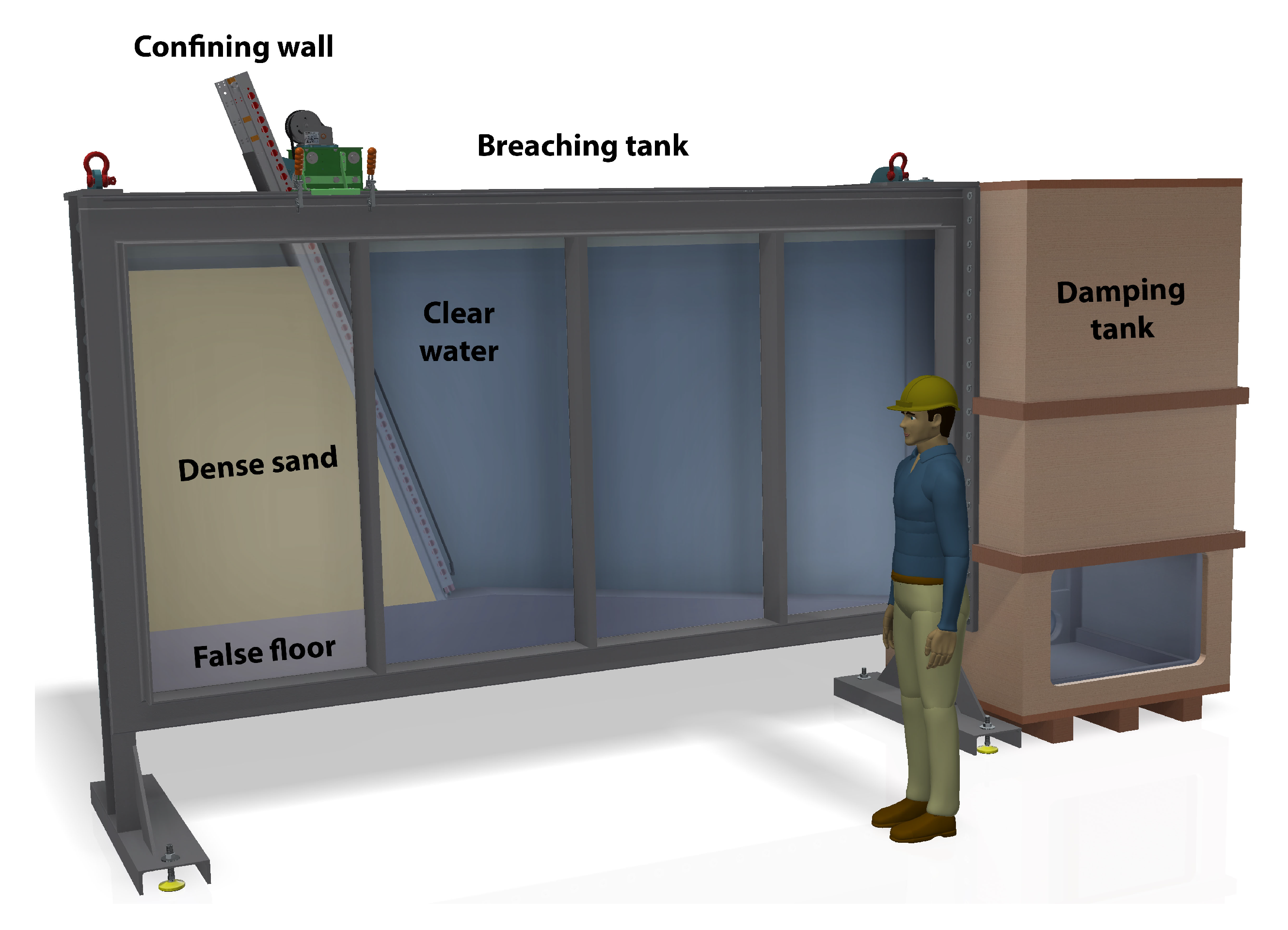
To evaluate the applicability and reliability of the present numerical model, the laboratory experiments carried out by [18] are reproduced numerically and the results are compared. A recapitulation of the experimental set-up of [18] is provided as follows. The series of laboratory experiments were conducted in a breaching tank: 4 m long, 0.22 m wide and 2 m high. The front wall of the tank was made of glass, whereas the back wall was made of steel. A sand deposit of a steep slope (50${}^{\circ }$–80${}^{\circ }$) was constructed under water. Owing to the over-steepening of the subaqueous slope, it was essentially unstable and, therefore, it was supported by a confining wall, which should be removed to kick-start the breaching failure and subsequently the turbidity current. The length of the breach face in all experiments did not exceed 1.6 m.

In the breaching tank, a false floor of a mild slope, compared to the breach face, was placed next to the slope toe, where the turbidity current made a turn (see Figure 2). To avoid the reflection of the turbidity current at the end of the downstream region, sand-water mixture was drained constantly during the experiment, while clear water of the same rate was supplied into the tank, so as to guarantee a constant water level.

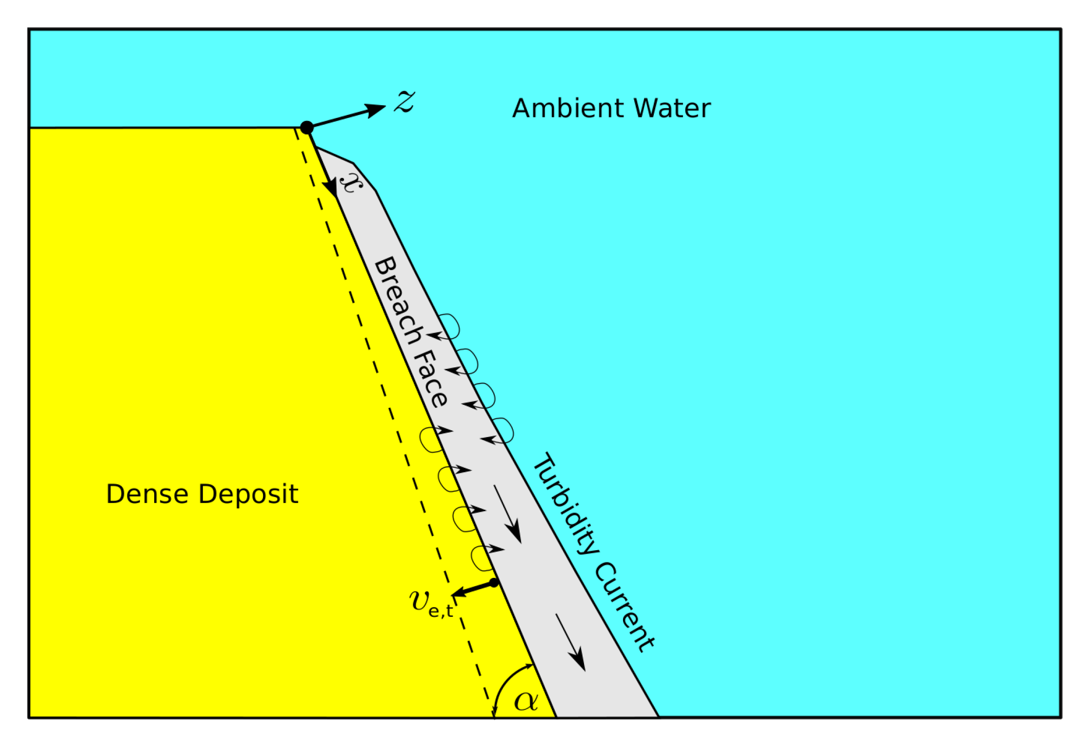
The work of [18] did not include measurements for the turbidity current flowing down the toe of the breach face. Therefore, the present simulations consider the breach face and the current running over it, and do not include a slope transition (see Figure 3). The sand used in the experiments ($d_{50}$ = 0.135 mm) was uniformly graded. Therefore, the simulations were run using a uniform particle size fraction of 0.135 mm.

Table 1. The properties of the sand used in the experiments [18].

${\mathbf{d}}_{50}$	${\mathit{n}}_0$	${\mathit{n}}_{\mathit{l}}$	$\mathit{\varphi }$	${\mathit{k}}_{\mathit{l}}$
0.135 mm	0.40	0.51	36${}^{\circ }$	0.0307 cm/s

summarizes the sand properties needed for the numerical computations.

A rectangular numerical flow domain is used, which follows the sloping bed. See Section 4.2 for details on the computational domain and grid. The gravity vector is rotated to account for a correct gravity pull on the density current, and sediment settling takes place along the rotated gravity vector. In the lab experiments, the bed erodes and moves backward with a rate equal to the erosion velocity. In the numerical simulations, there is no bed update and the bed does not move backward, but the erosion velocity (∼mm/s) is prescribed as an inflowing boundary condition at the bed. At the free surface, a rigid lid free slip condition is prescribed.

The flow is internally generated in the computational domain and no inflow or outflow is prescribed at the lateral, left or right end. This will result in a flow reflection at the right wall after some time, but a sufficiently large domain is chosen, and the simulations are stopped before that happens. The width of the domain is equal to the experimental width and closed lateral boundary conditions are applied with a partial slip boundary condition employing a wall roughness $k_n=0.2$ mm to account for wall resistance of the current.

4.1. Model Inputs

Some inputs are needed to run the simulations, such as slope angle, slope length and sand properties. The initial conditions of the numerical runs are summarized in

Table 2. Initial conditions of the numerical runs.

Run #	Slope Angle (${}^{\circ }$)	Pure Breaching (mm/s)	${\mathit{f}}_{\mathit{cr}}$	${\mathit{n}}_0$
1	50	0.28 ${}^a$	1.06	0.40
2	54	0.37 ${}^b$	1.10	0.40
3	64	0.58 ${}^a$	1.22	0.40
4	67	0.82 ${}^b$	1.27	0.40
5	70	0.92 ${}^b$	1.31	0.40
6	77	1.20 ${}^b$	1.43	0.40
7	81	1.35 ${}^a$	1.50	0.40
8	67	1.21 ${}^b$	1.27	0.44

${}^a$ Experimental data, ${}^b$ calculated using Equation (14) (not available in corresponding experiments).

. Upon the start of the numerical simulations, a discharge of sediment-water mixture equivalent to the corresponding pure breaching is introduced to the numerical domain at the first computational grid cell above the bed. Thereupon, the turbidity current starts developing along the breach face.

4.2. Computational Grid

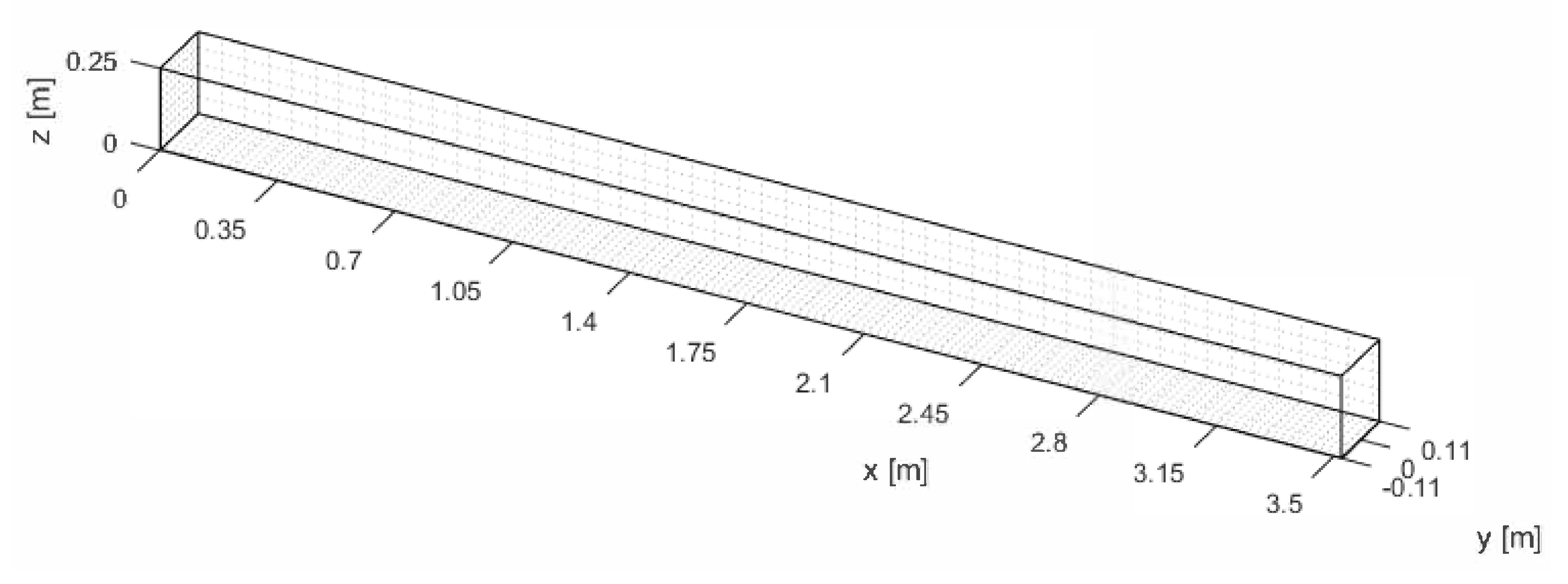
The computational geometry used in the simulations is demonstrated in Figure 4. The domain height is 25 cm, deep enough to avoid effects of the overflow above the turbidity current, while the domain width is 22 cm, equal to the width of the experimental setup. As the purpose of the numerical simulations is to reproduce the current running along the breach face (1.5 m long), it was decided to have a total domain length of 3.5 m. The domain is divided into two zones. The first zone (0 to 1.8 m) corresponds to the breach face over which the turbidity current propagates. The second zone (1.8 m to 3.5 m) functions as a sediment sink, where the sand particles settle out, decelerating the flow and preventing the reflection of the turbidity current upstream. The numerical data after x = 1.5 m are not considered, since they are influenced by the sediment sink.

The computational mesh consists of a total number of about 46 million cells. To reduce the computational time, grid clustering was used in x-direction; a width of 2 mm was used for the cells in the first 1.5 m, while the width of the remaining cells was gradually increased with a growth rate of 1.04 with an upper limit of 5 cm. The cell dimensions in the y and z directions were kept constant with a value of 2 mm and 0.5 mm, respectively (leading to maximum $\Delta z^{+}=15$ for the first velocity point located at $\frac{1}{2}\Delta z$). The average computational time of the runs presented in this study was about 4 days.

5. Model Validation

As noted earlier, the WALE sub-grid-scale model is used in this study. To ensure that the numerical results are independent of the chosen sub-grid-scale model, an extra simulation has been run using the dynamic Smagorinsky sub-grid-scale model (which is more computationally demanding) and the simulation results were compared with those obtained with the WALE sub-grid-scale model. Indeed, no differences have been observed between the results.

In this section, specific quantitative time-averaged numerical results are compared with the corresponding experimental results to test the validity and reliability of the proposed numerical model. However, some instantaneous flow results are first presented to illustrate the type of flow we are dealing with.

5.1. Instantaneous Flow Results

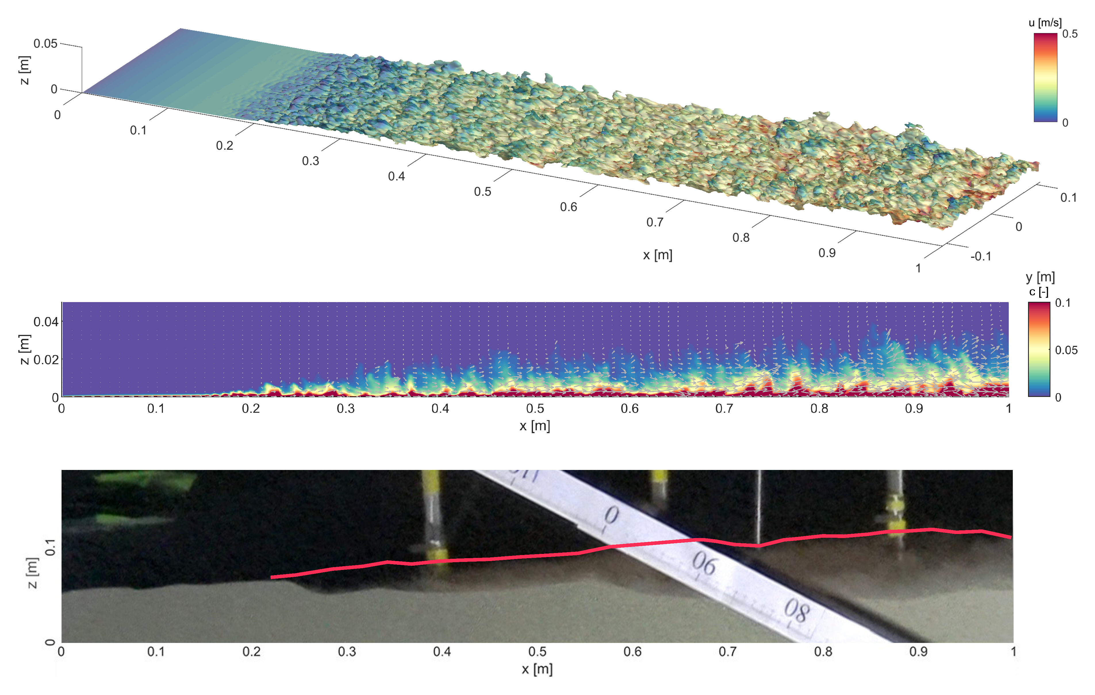
In general, turbidity currents are known to be highly turbulent and breaching-generated turbidity current is not an exception. Figure 5 clearly shows the transition of the flow from laminar to turbulent at about x = 20 cm for the 64${}^{\circ }$ slope, which is in line with visual observations during the experiment. The top plot demonstrates the 3D high turbulent behavior of the turbidity current while the middle plot illustrates the highly turbulent instantaneous concentration and velocity distribution over the vertical. The latter also shows that the inner region is very thin compared to the total layer thickness and that significant velocities can be found in zones with relative low sediment concentrations between 0.01$<c<$0.1. In the remainder of this section, time-averaged model results are used in the comparison with the experimental results.

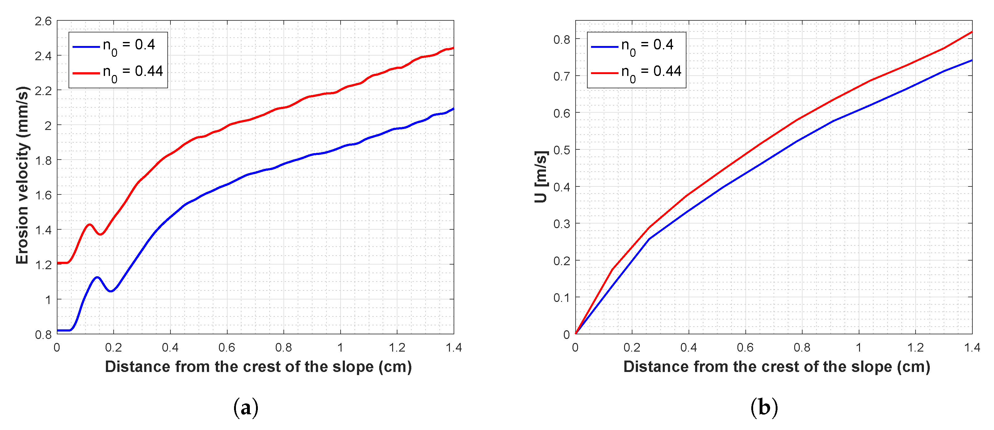
5.2. Sediment Erosion

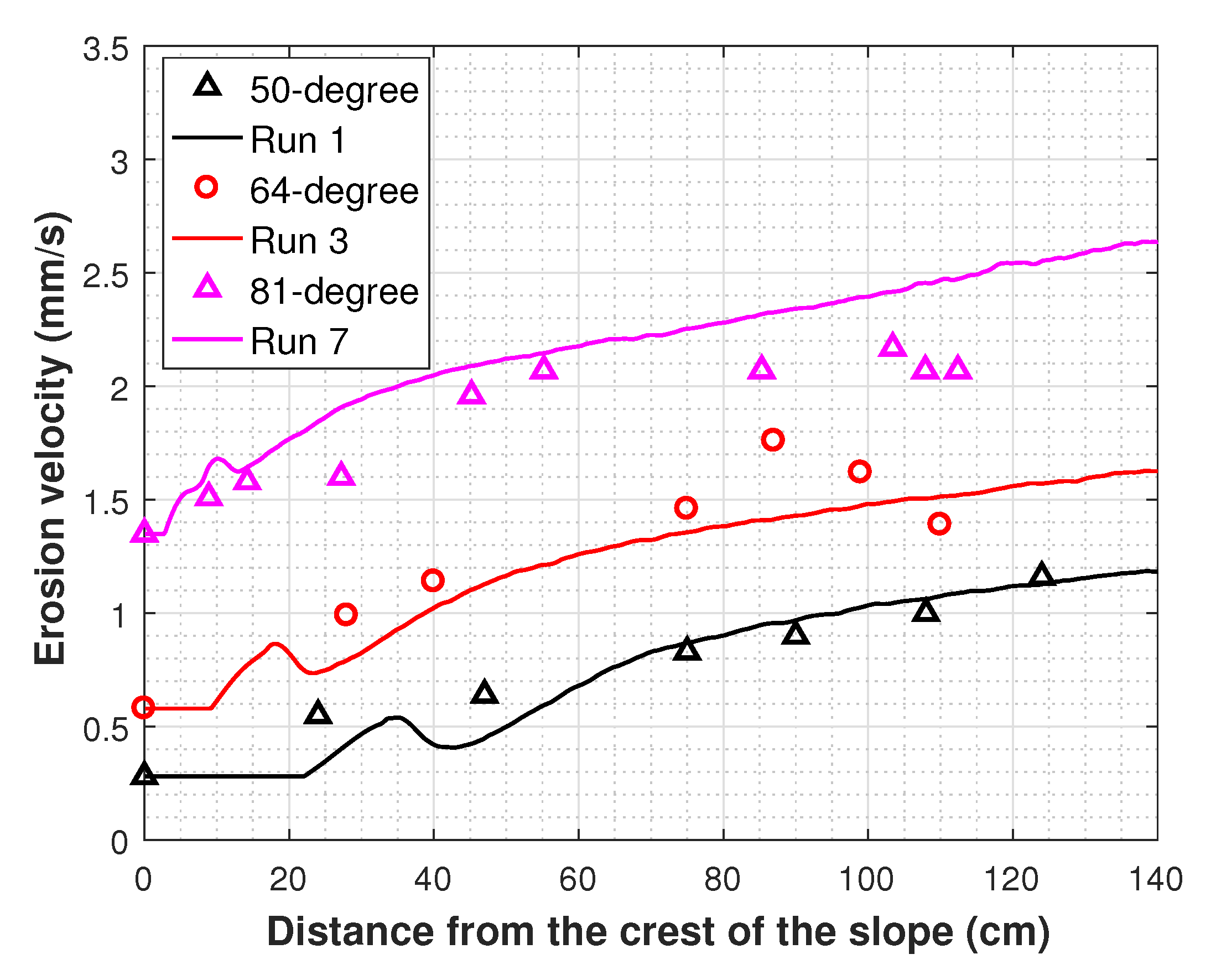
To evaluate the proposed breaching erosion model and the morphodynamic response associated with the turbidity currents, simulation results are compared against the corresponding experimental data (see Figure 6). For each of the numerical runs, the constructed erosion velocities are the average magnitudes over a 3-second time span and a lateral distance of the first 10% of the domain width (2.2 cm). This is because the erosion velocities reported in [18] were computed from the video recordings filmed through the glass wall.

As it can be seen, the numerically predicted erosion velocities coincide very well with the experimental data. The prediction accuracy of the erosion model is considered high (mean absolute error = 11%) compared to the acceptable accuracy in the field of sediment transport. The erosion lines in Figure 6 begin with a horizontal segment, where the turbidity current is not yet sufficiently energetic to erode sediment from the breach face. Shortly after that, the turbidity current ignites and increasingly erodes sediments from the breach face.

The experimental data suggests a transition in the erosion rate after a certain point. For example, in the case of the 81${}^{\circ }$ breach face, the observed erosion velocity is found to be almost constant in the streamwise distance 55–110 cm. It could be that the in situ porosity $n_0$ was not uniform all over the breach face (see Section 6.6 for the effect of $n_0$). Another hypothesis is that the current was in the bypass mode (the current maintains the sediment load), but that is not captured in the numerical model. This may be attributed to the reference line of the near-bed concentration, which should be defined based on the dimensions of the turbulent eddies transporting the sand grains from the turbidity current back to the breach face. The size of those eddies was not considered in [18] as that requires experimental data of higher resolution.

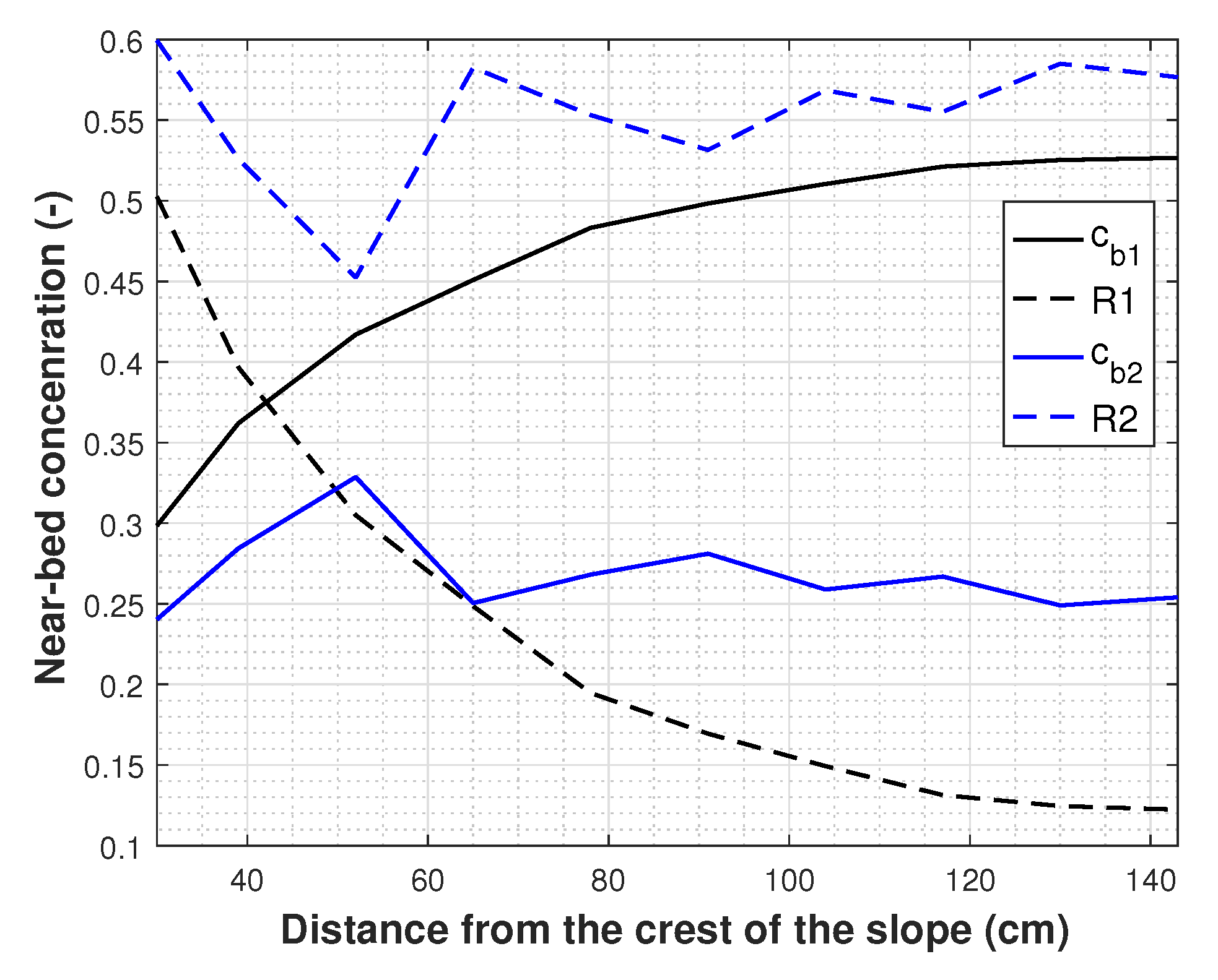
To elaborate on this hypothesis, we show in Figure 7 two different definitions of the near-bed concentration $c_b$ and the corresponding reduction factor R; $c_{b1}$ is the concentration of the first cell above the bed, while $c_{b2}$ is the average concentration in the inner region. The value of $c_{b2}$ tends to become constant downslope and consequently the reduction factor $R_2$ also remains constant. In contrast, $c_{b1}$ rapidly increases in the downstream direction and hence the reduction factor $R_1$ rapidly decreases. This implies that at some point along the breach face, the increase in bed shear stress will be balanced by the increase of the near-bed concentration, transforming the flow from the self-acceleration mode to the bypass mode. In conclusion, the definition of the near-bed concentration influences the computed erosion rates and, consequently, might influence the flow mode.

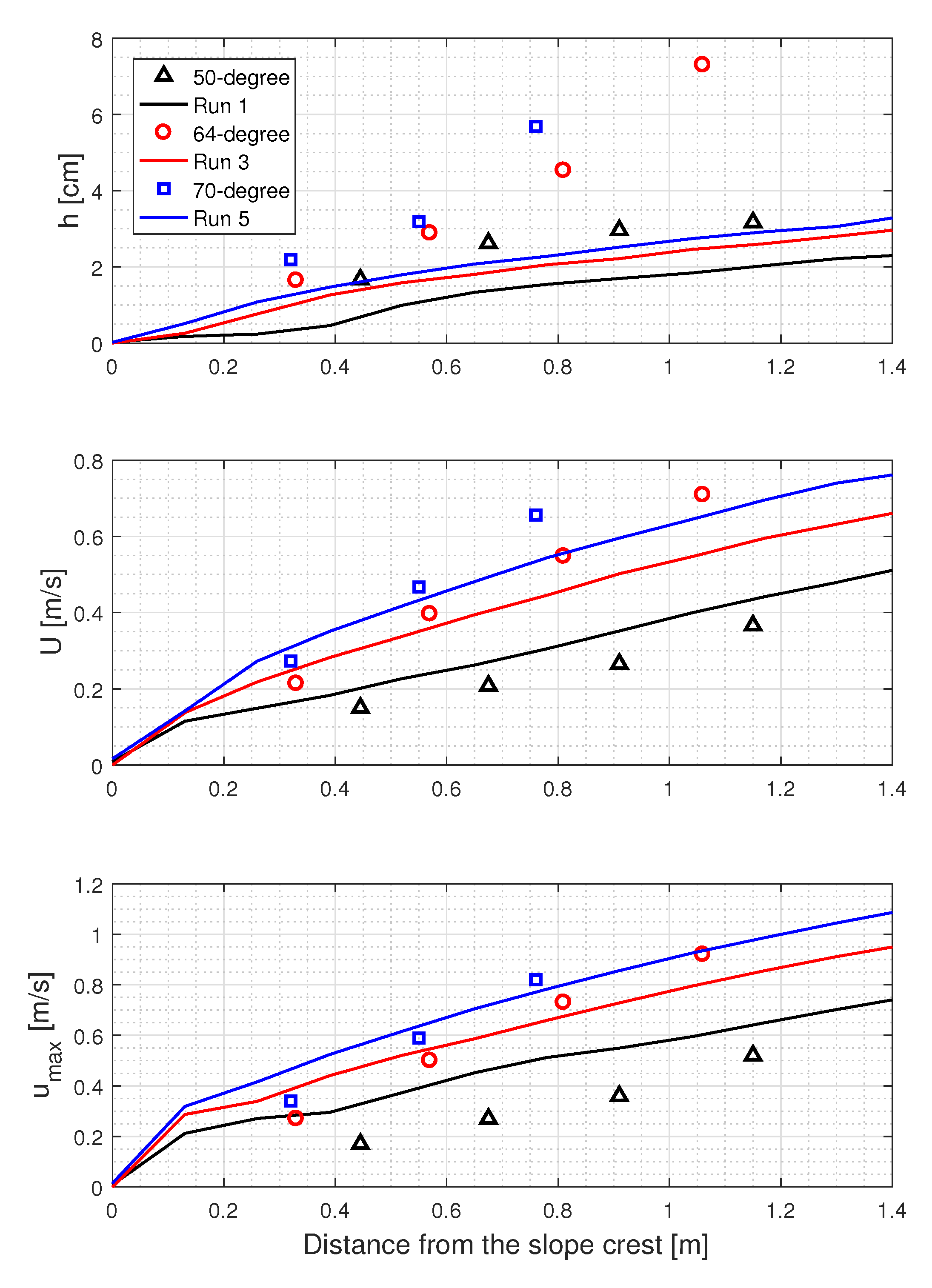
5.3. Flow Spatial Evolution

The characterizing layer thicknesses h and depth-averaged velocities U for Run 1, Run 3 and Run 5 are constructed and compared with corresponding magnitudes derived from the laboratory experiments. These flow characteristics, h and U, are calculated using the following relationships [14,26,54]:

$$Uh={\int }_0^{z_{\infty }}udz,$$

(20)

$$U^{2}h={\int }_0^{z_{\infty }}{u}^{2}dz,$$

(21)

where u is locally averaged streamwise flow velocity, z is upward-normal distance from the bed and $z_{\infty }$ is the height at which the local velocity u is zero.

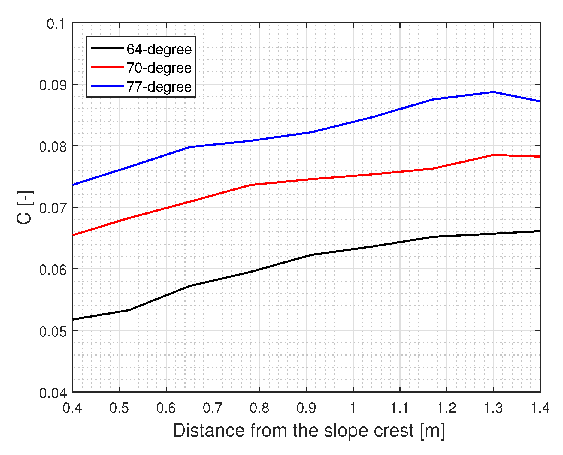
In these runs, the densimetric Froude number is greater than one, indicating that the flow is supercritical, which agrees with the experimental results. The densimetric Froude number is calculated using the following relationship [55]:

$$F{r}_d=\frac{U}{\sqrt{\Delta gCh}},$$

(22)

where C denotes the layer-averaged, volume concentration of sediment defined as:

$$C=\frac{{\int }_0^{z_{\infty }}cudz}{{\int }_0^{z_{\infty }}udz},$$

(23)

in which c is local concentration of suspended sediment.

In addition to the characteristics h and U, the layer-peak velocities $u_{max}$ are also constructed in Figure 8. It can be seen that the model predictions of the spatial evolution of the flow agree qualitatively with the experimental data. However, the model fails to accurately predict the layer thickness (mean absolute error = 46%); it is underestimated. We speculate that this underestimation partly relates to the missing feedback from the sand particles to the flow, leading to less momentum exchange and mixing. This underestimation could be one of the reasons for the deviation between the numerically predicted layer-averaged velocities and the experimental ones (mean absolute error = 18%); the predicted flow velocities for the 64${}^{\circ }$ and 70${}^{\circ }$ breach faces are somewhat lower than the measured ones. Another important reason for this difference is that the coupled erosion model was calibrated based on the erosion rates measured at the glass wall of the experimental tank. However, Alhaddad et al. [18] found the erosion to be the highest in the middle of the tank width, where the velocity measurements were obtained, declining towards the side walls. This implies that somewhat more sediment should be entrained from the breach face to the turbidity current to gain higher velocities.

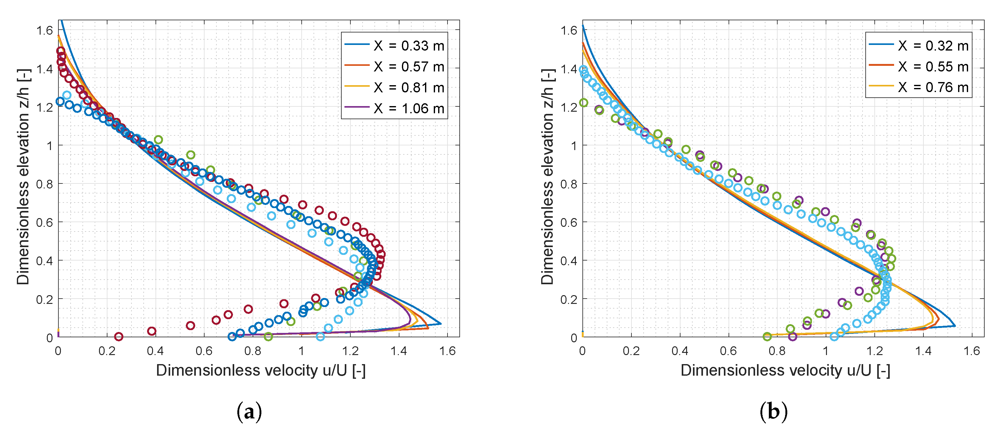
5.4. Vertical Structure

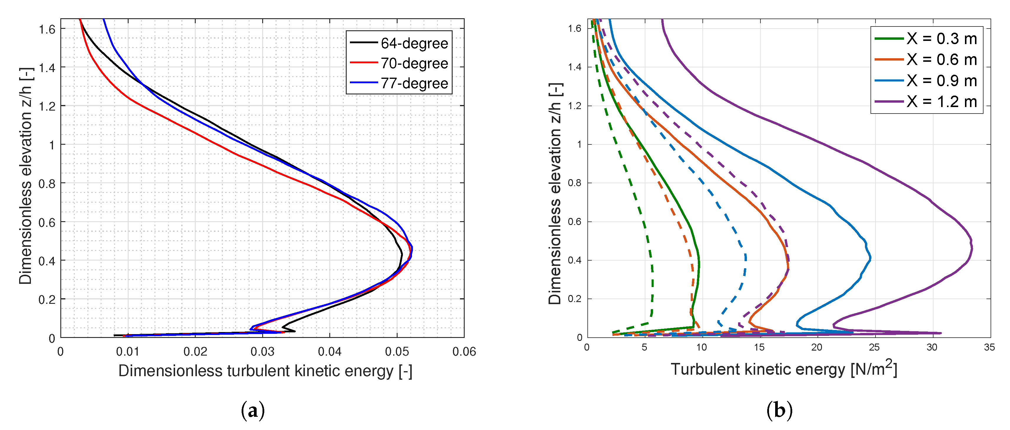
The non-dimensional vertical profiles of the streamwise velocities for Run 3 and Run 5 are constructed and compared with the corresponding dimensionless profiles derived from the laboratory experiments. In these numerical runs, the profiles are taken at the same distances from the breach crest as in the experiments. The streamwise local velocities are normalized with the depth-averaged velocity U, while the local vertical distances are normalized with the characterizing layer thickness h.

Overall agreement is found between simulation and experimental results in the vertical structure (see Figure 9), but simulation predictions deviate from experiments in the location of the velocity maximum $u_{max}$. The latter is numerically predicted to be closer to the bed than measured in the experiments, leading to an over-predicted velocity gradient in the inner region. This could be partially attributed to the underestimation of the layer thicknesses by the model. Another possible reason for the differences is the difficulties and uncertainties in pinpointing the bed position in the laboratory experiments, as stated in the work of [18]. The numerical results demonstrate that the velocity profiles are self-similar, as can be inferred from the experimental results [18].

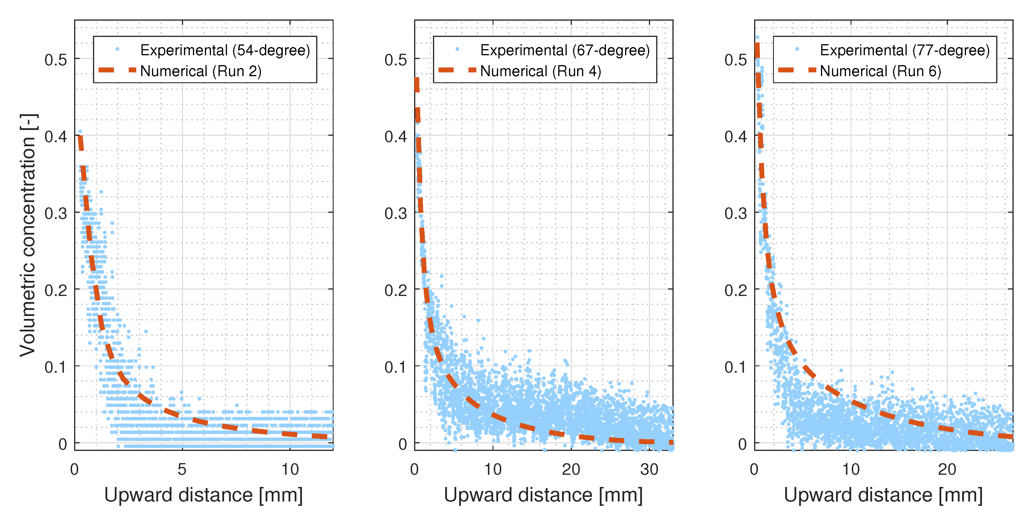
5.5. Vertical Density Distribution

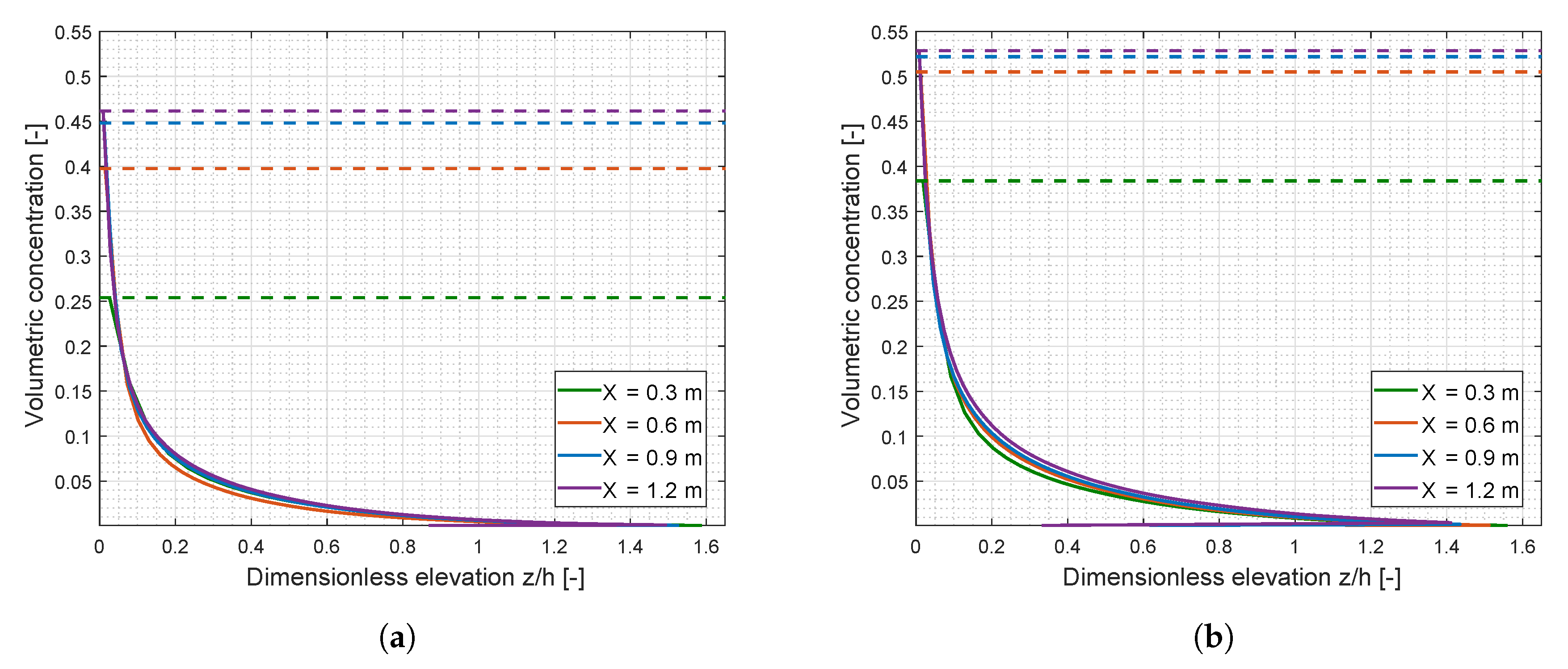
We examine here the capability of the model to capture the internal density distribution of the flow through comparing concentration profiles measured with Conductivity-type Concentration Meter (CCM) (single-point device) along different inclinations versus numerical results. It can be seen from Figure 10 that the time-averaged concentration profiles predicted by the model fall within the scatter range of the corresponding profiles resulted from the laboratory experiments. Also, the very high near-bed concentrations in the order of c = 0.4–0.52 are captured in the numerical model. This indicates that the numerical model can adequately predict the vertical density distribution of the considered turbidity current.

5.6. Conclusion on Comparison of Numerical Simulations and Experiments

In view of the presented systematic comparison between the numerical and experimental results, it can be concluded that the numerical model gives fairly reasonable predictions of the flow characteristics and the associated morphodynamic response. In the next section, therefore, we investigate further flow characteristics, which were not possible to analyze through the experimental data.

6. Further Analysis of Numerical Results

In Section 5 we showed that the model was good at simulating the experimental observations. This gives us confidence to closely investigate the flow and turbulence structure, to determine some characterizing parameters and to analyze the sensitivity of the numerical results to some initial conditions. This will be the scope of this section.

6.1. Layer-Averaged Concentration

Figure 11 depicts the spatial development of the layer-averaged concentration C (Equation (23)) for three slope angles. Clearly, steeper slopes result in a higher C owing to the higher sediment erosion. The results show that C increases in the downstream direction, in the same manner as the layer-averaged velocity U (see Figure 8). This supports the conclusion drawn by [18] that breaching-generated turbidity currents are self-accelerating. According to [56], self-accelerating flow is characterized by the downstream increase of flow velocity, which is caused by downstream increase in suspended sediment concentration.

6.2. Spatial Evolution of Vertical Density Distribution

The vertical profiles of the sediment concentrations for Run 3 and Run 6 are depicted in Figure 12. As the flow further travels downslope, the near-bed concentration increases. Moreover, steeper slopes result in higher near-bed concentrations, which can be attributed to the higher erosion rates caused by a larger gravity force and more erosive turbidity currents.

6.3. Reynolds Stresses

The Reynolds stress distribution corresponds to the velocity gradient within the flow body as maximum stresses occur where the gradient is largest. The normal Reynolds stresses can be obtained from the turbulent fluctuations of downstream $u^{\prime }$ and bed-normal velocity $w^{\prime }$ as follows:

$${\tau }_r=-\rho \overline{u^{\prime }{w}^{\prime }}.$$

(24)

The Reynolds stresses are calculated using the turbulent velocity components averaged over a 3-second time span. For three different slopes at x = 1 m, Reynolds stresses are normalized by $\rho U^2$ and their distribution is shown in Figure 13a. The Reynolds stress increases significantly near the breach face, reaching the largest positive Reynolds stress at z/h ∼ 0.025, where the bottom boundary layer ends. Around and below the velocity maximum, z/h = 0.045–0.085, Reynolds stresses are close to zero. Further upwards, in the outer region of the flow, where the velocity gradient is negative, Reynolds stresses become negative, reaching the largest negative Reynolds stress at z/h ∼ 0.45. This elevation has the largest negative velocity gradient. Above this elevation, Reynolds stresses decreases towards nearly zero at the upper boundary of the flow. It is found that Reynolds stresses take a self-similar shape.

Figure 13c illustrates the spatial development of Reynolds stresses along 64${}^{\circ }$ and 77${}^{\circ }$ breach faces. Owing to the acceleration of the flow downslope, the flow becomes more turbulent, leading to higher Reynolds stresses in the downstream direction. These stresses, as can be seen in Figure 13c, are higher for steeper breach faces, as these result in higher flow velocities.

6.4. Turbulent Kinetic Energy

Profiles of turbulent kinetic energy (TKE) are constructed to analyze the vertical distribution of the TKE within the flow. The total TKE is calculated using the turbulent velocity components averaged over a 3-second time span as follows

$$TKE=\frac{1}{2}\rho (\overline{{u^{\prime }}^2}+\overline{{v^{\prime }}^2}+\overline{{w^{\prime }}^2}),$$

(25)

where $u^{\prime }$ is the streamwise component, $v^{\prime }$ is the across-stream component and $w^{\prime }$ is bed-normal component. Numerical TKE normalized by $\rho U^2$ is plotted in Figure 14a for three different slope angles at x = 1 m. The TKE profiles show a significant increase of TKE in the bottom boundary layer z/h ∼ 0–0.025 and then a decrease until z/h ∼ 0.045, a little below the velocity maximum. Above the elevation of the velocity maximum, the TKE increases again, reaching the largest TKE at z/h ∼ 0.45, coinciding with the largest negative velocity gradient and largest Reynolds stress. Above this elevation, TKE tends to decrease towards the upper boundary of the flow. The results suggest that TKE takes a self-similar shape.

Figure 14b illustrates the spatial development of TKE along 64${}^{\circ }$ and 77${}^{\circ }$ breach faces. In a similar way to the Reynolds stresses, the TKE increases downslope and is higher for steeper slopes.

6.5. Bed Shear Stress and Bed Friction Coefficient

The bed shear stress ${\tau }_b$ determines the erosive power of the flow and can be expressed in terms of a bed friction coefficient $C_f$, which relates the bed shear velocity $u_{*}$ to the layer-averaged velocity U as follows

$$C_f=\frac{u_{*}^2}{U^2}$$

(26)

This relation is usually used in depth-averaged models. These are more computationally efficient and can be used to make some preliminary computations. In this study, the value of $u_{*}$ is calculated using Equation (11). The average value of the $C_f$ is calculated here from the numerical results.

The calculated values of $C_f$ show that the bed friction coefficient is not a constant parameter (Figure 15); it decreases downslope. This is because the thickness of the current increases along the streamwise direction, resulting in an increased bulk Reynolds number and, consequently, a decreased drag coefficient. The results also show that steeper slopes lead to a lower bed friction coefficient. For the considered slope angles and traveling distance, $C_f$ ranges from 0.028 to 0.006 with an average value of 0.011. This is consistent with the range of values reported in the literature (e.g., [54]).

6.6. Influence of In Situ Porosity

The experiments of [18] were all conducted using a constant sand in situ porosity $n_0$ = 0.4. To investigate the effect of $n_0$ on the flow and erosion velocity, an additional numerical simulation for 67${}^{\circ }$ breach face was run using $n_0$ = 0.44, which corresponds to a sand relative density of 68%. A comparison between the numerical results for $n_0$ = 0.4 (Run 4) and $n_0$ = 0.44 (Run 8) is shown in Figure 16. It can be seen from Figure 16a that higher $n_0$ results in higher pure breaching and hence higher erosion velocities downslope; the average increase in erosion, in the considered case, is significant (47%). Higher $n_0$ leads to a lower hydraulic gradient (which acts as a stabilizing force) during shearing, increasing the erosion velocity. As a result, the flow becomes denser and runs faster downslope, as depicted in Figure 16b. The difference of the layer-averaged velocities between the two runs is magnified downstream.

7. Conclusions

We use a 3D numerical model to conduct large eddy simulations of turbidity currents generated during breaching flow slides. The qualitative and quantitative comparison between experimental and simulation results indicates that the proposed numerical tool can reasonably reproduce several substantial aspects of the flow, such as vertical density distribution, and spatial development down the breach face. A limitation of the model is that it underestimates the thickness of the current. Considering the special conditions of breaching, a new breaching erosion model is proposed and verified through published experimental data. Good agreement is observed between the experimental and numerically predicted erosion rates. The numerical results confirm the self-accelerating behavior of breaching-generated turbidity currents. Both Reynolds stresses and TKE decrease sharply below their maximum in the bottom boundary layer. In addition, the numerical results reveal that breaching-generated turbidity currents exhibit a self-similar behavior; velocity, concentration, Reynolds stress, and TKE profiles take a self-similar shape. Based on a sensitivity analysis, sand erosion during breaching is found to be susceptible to the in situ porosity; the lower the in situ porosity, the higher the sand resistance to erosion. If the present numerical model is extended to account for the morphological changes of the breach face, it would serve as a good tool to predict the breaching evolution and stability.

References

1. Salinas, J.S.; Cantero, M.; Shringarpure, M.; Balachandar, S. Properties of the Body of a Turbidity Current at Near-Normal Conditions: 1. Effect of Bed Slope. J. Geophys. Res. Ocean. 2019, 124, 7989–8016. [Google Scholar] [CrossRef]
2. Hage, S.; Cartigny, M.J.; Sumner, E.J.; Clare, M.A.; Hughes Clarke, J.E.; Talling, P.J.; Lintern, D.G.; Simmons, S.M.; Silva Jacinto, R.; Vellinga, A.J.; et al. Direct monitoring reveals initiation of turbidity currents from extremely dilute river plumes. Geophys. Res. Lett. 2019, 46, 11310–11320. [Google Scholar] [CrossRef] [Green Version]
3. Alhaddad, S.; Labeur, R.J.; Uijttewaal, W. Breaching Flow Slides and the Associated Turbidity Current. J. Mar. Sci. Eng. 2020, 8, 67. [Google Scholar] [CrossRef] [Green Version]
4. Paull, C.K.; Talling, P.J.; Maier, K.L.; Parsons, D.; Xu, J.; Caress, D.W.; Gwiazda, R.; Lundsten, E.M.; Anderson, K.; Barry, J.P.; et al. Powerful turbidity currents driven by dense basal layers. Nat. Commun. 2018, 9, 1–9. [Google Scholar] [CrossRef] [Green Version]
5. Parsons, J.D.; Bush, J.W.; Syvitski, J.P. Hyperpycnal plume formation from riverine outflows with small sediment concentrations. Sedimentology 2001, 48, 465–478. [Google Scholar] [CrossRef]
6. Normandeau, A.; Lajeunesse, P.; St-Onge, G.; Bourgault, D.; Drouin, S.S.O.; Senneville, S.; Bélanger, S. Morphodynamics in sediment-starved inner-shelf submarine canyons (Lower St. Lawrence Estuary, Eastern Canada). Mar. Geol. 2014, 357, 243–255. [Google Scholar] [CrossRef]
7. Hizzett, J.L.; Hughes Clarke, J.E.; Sumner, E.J.; Cartigny, M.; Talling, P.; Clare, M. Which triggers produce the most erosive, frequent, and longest runout turbidity currents on deltas? Geophys. Res. Lett. 2018, 45, 855–863. [Google Scholar] [CrossRef] [Green Version]
8. Mastbergen, D.R.; Beinssen, K.; Nédélec, Y. Watching the Beach Steadily Disappearing: The Evolution of Understanding of Retrogressive Breach Failures. J. Mar. Sci. Eng. 2019, 7, 368. [Google Scholar] [CrossRef] [Green Version]
9. Van Den Berg, J.H.; Van Gelder, A.; Mastbergen, D.R. The importance of breaching as a mechanism of subaqueous slope failure in fine sand. Sedimentology 2002, 49, 81–95. [Google Scholar]
10. Alhaddad, S.; Labeur, R.J.; Uijttewaal, W. The need for experimental studies on breaching flow slides. In Proceedings of the Second International Conference on the Material Point Method for Modelling Soil-Water-Structure Interaction, Cambridge, UK, 8–10 January 2019; pp. 166–172. [Google Scholar]
11. Eke, E.; Viparelli, E.; Parker, G. Field-scale numerical modeling of breaching as a mechanism for generating continuous turbidity currents. Geosphere 2011, 7, 1063–1076. [Google Scholar] [CrossRef]
12. Inman, D.L.; Nordstrom, C.E.; Flick, R.E. Currents in submarine canyons: An air-sea-land interaction. Annu. Rev. Fluid Mech. 1976, 8, 275–310. [Google Scholar] [CrossRef]
13. Talling, P.J.; Paull, C.K.; Piper, D.J. How are subaqueous sediment density flows triggered, what is their internal structure and how does it evolve? Direct observations from monitoring of active flows. Earth-Sci. Rev. 2013, 125, 244–287. [Google Scholar] [CrossRef] [Green Version]
14. Garcia, M.; Parker, G. Experiments on the entrainment of sediment into suspension by a dense bottom current. J. Geophys. Res. Ocean. 1993, 98, 4793–4807. [Google Scholar] [CrossRef]
15. Kneller, B.C.; Bennett, S.J.; McCaffrey, W.D. Velocity structure, turbulence and fluid stresses in experimental gravity currents. J. Geophys. Res. Ocean. 1999, 104, 5381–5391. [Google Scholar] [CrossRef]
16. Stagnaro, M.; Pittaluga, M.B. Velocity and concentration profiles of saline and turbidity currents flowing in a straight channel under quasi-uniform conditions. Earth Surf. Dyn. 2014, 2, 167. [Google Scholar] [CrossRef] [Green Version]
17. Ottolenghi, L.; Cenedese, C.; Adduce, C. Entrainment in a dense current flowing down a rough sloping bottom in a rotating fluid. J. Phys. Oceanogr. 2017, 47, 485–498. [Google Scholar] [CrossRef] [Green Version]
18. Alhaddad, S.; Labeur, R.J.; Uijttewaal, W. Large-scale Experiments on Breaching Flow Slides and the Associated Turbidity Current. J. Geophys. Res. Earth Surf. 2020, 125, e2020JF005582. [Google Scholar] [CrossRef]
19. Ottolenghi, L.; Adduce, C.; Inghilesi, R.; Armenio, V.; Roman, F. Entrainment and mixing in unsteady gravity currents. J. Hydraul. Res. 2016, 54, 541–557. [Google Scholar] [CrossRef]
20. Nourazar, S.; Safavi, M. Two-Dimensional Large-Eddy Simulation of Density-Current Flow Propagating up a Slope. J. Hydraul. Eng. 2017, 143, 04017035. [Google Scholar] [CrossRef]
21. Pelmard, J.; Norris, S.; Friedrich, H. LES grid resolution requirements for the modelling of gravity currents. Comput. Fluids 2018, 174, 256–270. [Google Scholar] [CrossRef]
22. Kyrousi, F.; Leonardi, A.; Roman, F.; Armenio, V.; Zanello, F.; Zordan, J.; Juez, C.; Falcomer, L. Large Eddy Simulations of sediment entrainment induced by a lock-exchange gravity current. Adv. Water Resour. 2018, 114, 102–118. [Google Scholar] [CrossRef]
23. Lucchese, L.V.; Monteiro, L.R.; Schettini, E.B.C.; Silvestrini, J.H. Direct Numerical Simulations of turbidity currents with Evolutive Deposit Method, considering topography updates during the simulation. Comput. Geosci. 2019, 133, 104306. [Google Scholar] [CrossRef]
24. Mastbergen, D.R.; Van Den Berg, J.H. Breaching in fine sands and the generation of sustained turbidity currents in submarine canyons. Sedimentology 2003, 50, 625–637. [Google Scholar] [CrossRef]
25. Yeh, T.h.; Cantero, M.; Cantelli, A.; Pirmez, C.; Parker, G. Turbidity current with a roof: Success and failure of RANS modeling for turbidity currents under strongly stratified conditions. J. Geophys. Res. Earth Surf. 2013, 118, 1975–1998. [Google Scholar] [CrossRef] [Green Version]
26. Parker, G.; Fukushima, Y.; Pantin, H.M. Self-accelerating turbidity currents. J. Fluid Mech. 1986, 171, 145–181. [Google Scholar] [CrossRef]
27. De Wit, L.; Talmon, A.; Van Rhee, C. 3D CFD simulations of trailing suction hopper dredger plume mixing: Comparison with field measurements. Mar. Pollut. Bull. 2014, 88, 34–46. [Google Scholar] [CrossRef]
28. De Wit, L.; Talmon, A.; Van Rhee, C. 3D CFD simulations of trailing suction hopper dredger plume mixing: A parameter study of near-field conditions influencing the suspended sediment source flux. Mar. Pollut. Bull. 2014, 88, 47–61. [Google Scholar] [CrossRef]
29. De Wit, L.; van Rhee, C.; Talmon, A. Influence of important near field processes on the source term of suspended sediments from a dredging plume caused by a trailing suction hopper dredger: The effect of dredging speed, propeller, overflow location and pulsing. Environ. Fluid Mech. 2015, 15, 41–66. [Google Scholar] [CrossRef]
30. De Wit, L. 3D CFD Modelling of Overflow Dredging Plumes. Ph.D. Thesis, Delft University of Technology, Delft, The Netherlands, 2015. [Google Scholar]
31. De Wit, L. 3D CFD modelling of hopper sedimentation. In Proceedings of the CEDA Dredging Conference, Rotterdam, The Netherlands, 7–8 November 2019. [Google Scholar]
32. Manninen, M.; Taivassalo, V.; Kallio, S. On the Mixture Model for Multiphase Flow VTT Publications 288. In Technical Research Center of Finland; Julkaisija-Utgivare: Helsinki, Finland, 1996. [Google Scholar]
33. Van Rhee, C. On the Sedimentation Process in a Trailing Suction Hopper Dredger. Ph.D. Thesis, Delft University of Technology, Delft, The Netherlands, 2002. [Google Scholar]
34. Saremi, S. Density-Driven Currents and Deposition of Fine Materials. Ph.D. Thesis, Technical University of Denmark, Lyngby, Denmark, 2014. [Google Scholar]
35. Goeree, J. Drift-Flux Modeling of Hyper-Concentrated Solid-Liquid Flows in Dredging Applications. Ph.D. Thesis, Delft University of Technology, Delft, The Netherlands, 2018. [Google Scholar]
36. Shanmugam, G. Slides, slumps, debris flows, turbidity currents, and bottom currents: Implications. In Earth Systems and Environmental Sciences; Elsevier Online Module: Amsterdam, The Netherlands, 2018. [Google Scholar] [CrossRef]
37. Bagnold, R.A. Auto-suspension of transported sediment; turbidity currents. Proc. R. Soc. Lond. Ser. A Math. Phys. Sci. 1962, 265, 315–319. [Google Scholar]
38. Mulder, T.; Alexander, J. The physical character of subaqueous sedimentary density flows and their deposits. Sedimentology 2001, 48, 269–299. [Google Scholar] [CrossRef]
39. Richardson, Y.; Zaki, W. Sedimentation and Fluidization. Part I Trans. Inst. Chem. Eng. 1954, 32, 35–53. [Google Scholar]
40. Nicoud, F.; Ducros, F. Subgrid-Scale Stress Modelling Based on the Square of the Velocity Gradient Tensor. Flow Turbul. Combust. 1999, 62, 183–200. [Google Scholar] [CrossRef]
41. Harlow, F.H.; Welch, J.E. Numerical calculation of time-dependent viscous incompressible flow of fluid with free surface. Phys. Fluids 1965, 8, 2182–2189. [Google Scholar] [CrossRef]
42. De Wit, L.; van Rhee, C. Testing an improved artificial viscosity advection scheme to minimise wiggles in large eddy simulation of buoyant jet in crossflow. Flow Turbul. Combust. 2014, 92, 699–730. [Google Scholar] [CrossRef]
43. Dodd, M.S.; Ferrante, A. A Fast Pressure-Correction Method for Incompressible Two-Fluid Flows. J. Comput. Phys. 2014, 273, 416–434. [Google Scholar] [CrossRef]
44. Prosperetti, A.; Tryggvason, G. Computational Methods for Multiphase Flow; Cambridge University Press: Cambridge, UK, 2007. [Google Scholar]
45. Van Rhee, C. Slope failure by unstable breaching. In Proceedings of the Institution of Civil Engineers-Maritime Engineering; Thomas Telford Ltd.: London, UK, 2015; Volume 168, pp. 84–92. [Google Scholar]
46. Van den Berg, J.; Martinius, A.; Houthuys, R. Breaching-related turbidites in fluvial and estuarine channels: Examples from outcrop and core and implications to reservoir models. Mar. Pet. Geol. 2017, 82, 178–205. [Google Scholar] [CrossRef]
47. Van Rhee, C.; Bezuijen, A. The breaching of sand investigated in large-scale model tests. In Proceedings of the 26th International Conference on Coastal Engineering, Copenhagen, Denmark, 22–26 June 1998; pp. 2509–2519. [Google Scholar]
48. Breusers, H. Hydraulic excavation of sand. In Proceedings of the International Course in Modern Dreding, The Hague, The Netherlands, 5–10 June 1977. [Google Scholar]
49. Bisschop, F. Erosion of Sand at High Flow Velocities: An Experimental Study. Ph.D. Thesis, Delft University of Technology, Delft, The Netherlands, 2018. [Google Scholar]
50. Dey, S.; Debnath, K. Sediment pickup on streamwise sloping beds. J. Irrig. Drain. Eng. 2001, 127, 39–43. [Google Scholar] [CrossRef]
51. Van Rhee, C.; Talmon, A. Sedimentation and erosion of sediment at high solids concentration. In Proceedings of the 18th International Conference on Hydrotransport, Rio de Janeiro, Brazil, 22–24 September 2010; BHR Group: Cranfield, UK, 2010; pp. 211–222. [Google Scholar]
52. Van Rijn, L.C. Sediment pick-up functions. J. Hydraul. Eng. 1984, 110, 1494–1502. [Google Scholar] [CrossRef]
53. Lamb, M.P.; Dietrich, W.E.; Venditti, J.G. Is the critical Shields stress for incipient sediment motion dependent on channel-bed slope? J. Geophys. Res. Earth Surf. 2008, 113, F02008. [Google Scholar] [CrossRef] [Green Version]
54. Parker, G.; Garcia, M.; Fukushima, Y.; Yu, W. Experiments on turbidity currents over an erodible bed. J. Hydraul. Res. 1987, 25, 123–147. [Google Scholar] [CrossRef]
55. Komar, P.D. Hydraulic jumps in turbidity currents. Geol. Soc. Am. Bull. 1971, 82, 1477–1488. [Google Scholar] [CrossRef]
56. Sequeiros, O.E.; Mosquera, R.; Pedocchi, F. Internal Structure of a Self-Accelerating Turbidity Current. J. Geophys. Res. Ocean. 2018, 123, 6260–6276. [Google Scholar] [CrossRef]
Figure 1. Comparison between the predictive ability of the original (Equation (13)) [18] and empirically corrected (Equation (14)) relations of pure breaching: d 50 = 0.135 mm, n 0 = 0.40, n l = 0.51, ϕ = 36 and k l = 0.0307 cm/s.
Jmse 08 00728 g001
Figure 2. 3D sketch of the experimental setup illustrating all components excluding the sedimentation tank.
Jmse 08 00728 g002
Figure 3. Sketch for the case considered in the numerical simulations; v e , t is the total erosion velocity and α is the slope angle.
Jmse 08 00728 g003
Figure 4. Geometry used in all numerical simulations: Δ x = 2 mm–5 cm, Δ y = 2 mm and Δ z = 0.5 mm; the current travels from left to right and sand particles are removed from x = 1.8 m onward.
Jmse 08 00728 g004
Figure 5. An instantaneous 3D view of the isosurface c = 0.01 at time = 8 s (Run 3); colors indicate the magnitude of the streamwise velocity (top). An instantaneous 2D vertical slice at y = 0 at time = 8 s (Run 3); colors indicate the magnitude of the sediment concentration c and vectors indicate the magnitude and direction of the streamwise and bed-normal velocities in this plane (middle). An instantaneous, experimental side view of the spatial development of the flow over a 64 breach face [18]; the flow propagates from left to right and the red line corresponds to the visual upper boundary of the flow (bottom).
Jmse 08 00728 g005
Figure 6. Comparison of erosion velocities resulted from numerical simulations and lab experiments.
Jmse 08 00728 g006
Figure 7. Two definitions of near-bed concentration c b and the corresponding reduction factors R; c b 1 is the concentration of the first cell above the bed, while c b 2 is the average concentration in the inner region.
Jmse 08 00728 g007
Figure 8. Comparison of spatial evolution of turbidity currents propagating over 50 , 64 , and 70 slopes: layer thickness development (top), layer-averaged velocity (middle), and layer-peak velocity U max (bottom).
Jmse 08 00728 g008
Figure 9. Comparison of numerical dimensionless velocity profiles (solid lines) versus experimental data (circles): (a) 64 breach face; (b) 70 breach face.
Jmse 08 00728 g009
Figure 10. Comparison of time-averaged, upward, normal concentration profiles predicted by the present model against the corresponding experimental results; 54 (left), 67 (middle), and 77 breach face (right).
Jmse 08 00728 g010
Figure 11. Spatial development of the layer-averaged concentration C along the breach face.
Jmse 08 00728 g011
Figure 12. Composite plot of numerical concentration profiles spaced by a distance of 0.3 m: (a) 64 breach face (Run 3); (b) 77 breach face (Run 6); horizontal dashed lines refer to the concentration maximum.
Jmse 08 00728 g012
Figure 13. (a) Composite plot of normalized Reynolds stresses profiles at x = 1 m for different slope angles; (b) Composite plot of dimensionless velocity profiles at x = 1 m for different slope angles; (c) Composite plot of Reynolds stresses profiles spaced by a distance of 0.3 m: dashed lines correspond to 64 breach face and solid lines correspond to 77 breach face.
Jmse 08 00728 g013
Figure 14. (a) Composite plot of normalized TKE profiles at x = 1 m for different slope angles; (b) Composite plot of TKE profiles spaced by a distance of 0.3 m: dashed lines correspond to 64 breach face and solid lines correspond to 77 breach face.
Jmse 08 00728 g014
Figure 15. Spatial change of bed friction coefficient along the breach face.
Jmse 08 00728 g015
Figure 16. Comparison between numerical results for 67 breach face using different initial porosities n 0 (a) erosion velocity; (b) layer-averaged velocity.
Jmse 08 00728 g016