Ultra-High-Resolution Mapping of Posidonia oceanica (L.) Delile Meadows through Acoustic, Optical Data and Object-based Image Classification

Abstract

In this study, we present a framework for seagrass habitat mapping in shallow (5–50 m) and very shallow water (0–5 m) by combining acoustic, optical data and Object-based Image classification. The combination of satellite multispectral images-acquired from 2017 to 2019, together with Unmanned Aerial Vehicle (UAV) photomosaic maps, high-resolution multibeam bathymetry/backscatter and underwater photogrammetry data, provided insights on the short-term characterization and distribution of Posidonia oceanica (L.) Delile, 1813 meadows in the Calabrian Tyrrhenian Sea. We used a supervised Object-based Image Analysis (OBIA) processing and classification technique to create a high-resolution thematic distribution map of P. oceanica meadows from multibeam bathymetry, backscatter data, drone photogrammetry and multispectral images that can be used as a model for classification of marine and coastal areas. As a part of this work, within the SIC CARLIT project, a field application was carried out in a Site of Community Importance (SCI) on Cirella Island in Calabria (Italy); different multiscale mapping techniques have been performed and integrated: the optical and acoustic data were processed and classified by different OBIA algorithms, i.e., k-Nearest Neighbors’ algorithm (k-NN), Random Tree algorithm (RT) and Decision Tree algorithm (DT). These acoustic and optical data combinations were shown to be a reliable tool to obtain high-resolution thematic maps for the preliminary characterization of seagrass habitats. These thematic maps can be used for time-lapse comparisons aimed to quantify changes in seabed coverage, such as those caused by anthropogenic impacts (e.g., trawl fishing activities and boat anchoring) to assess the blue carbon sinks and might be useful for future seagrass habitats conservation strategies.

1. Introduction

1.1. Seagrass Habitat, Importance and Knowledge

Seagrass beds are distributed over a near-global extent and play an important role in coastal ecosystems as primary producers, providers of habitat and environmental structure, and shoreline stabilizers [1,2]. Seagrasses are considered one of the most important coastal habitats [3], as they support a wide range of ecologically and economically important marine species from different trophic levels [4]. Moreover, vegetated coastal ecosystems and especially seagrass meadows, are highly productive and have exceptional capacities to sequester carbon dioxide (CO₂) [5]. P. oceanica is an endemic Mediterranean species and is protected by specific European legislation frameworks such as the EU Habitat Directive (92/43/CEE) which includes P. oceanica beds among its priority habitats (Habitat Type 1120). Furthermore, according to the Water Framework Directive 2000/60/EC and the Marine Strategy Framework Directive (MFSD -2008/56/EC), P. oceanica is selected as a representative species among the angiosperm quality elements for evaluating “Good Ecological Status” and “Good Environmental Status” in the Mediterranean marine environments. Therefore, in order to protect this seagrass ecosystem, it is important to establish its preservation status and regularly monitor its abundance and distribution. Furthermore, the evaluation of its ecological status should be based on a monitoring strategy design that should be able to record accurately all its different spatial configurations (ranging from highly fragmented to continuous meadows) and arrangements, ranging across scales of meters to kilometers (seagrass landscapes), meters to tens of meters (patches), to tens of centimeters to meters (rhizomes, shoot groups) [6,7].

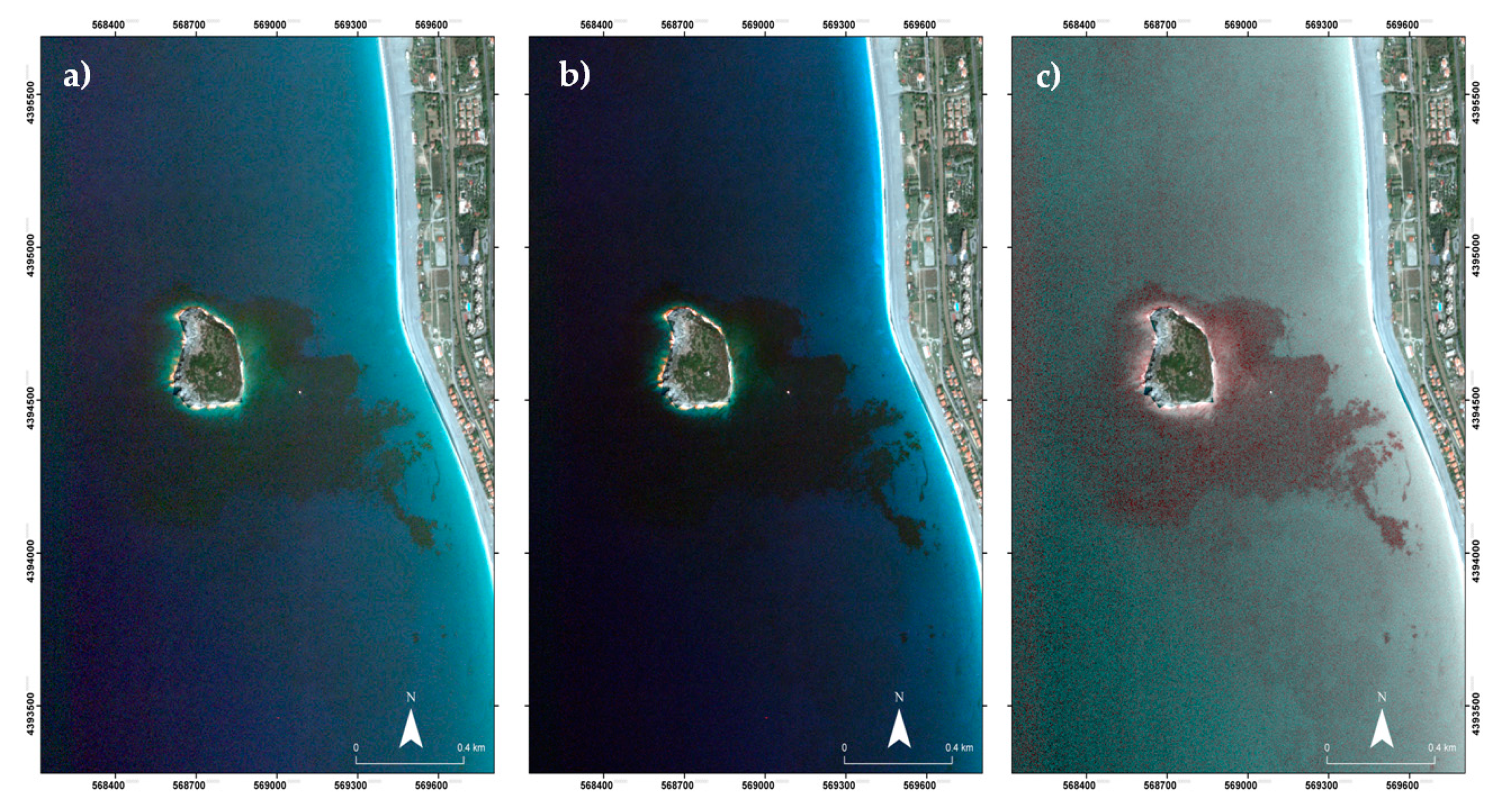
1.2. Application of Multispectral Satellite Systems in Seagrass Habitat Mapping

Remotely sensed aerial or satellite optical imagery has been used successfully by several authors to assess the spatial distribution and spatiotemporal changes in seagrass habitats [8,9,10,11,12,13,14] and has been proven to be suitable for mapping and monitoring seagrass ecosystems [14,15]. Seagrass detection with multispectral or hyperspectral imaging is one of the most widespread methods in this research area, since data collection is faster than other surveying techniques. Moreover, these techniques have lower costs, medium resolution accuracy, easier replicability and cover wider areas compared to traditional field-based methods [5]. However, they typically provide low-resolution images and even if remote technologies have a great potential in seabed mapping studies, the extraction of the bottom reflectance spectrum from the orbital optical sensors data is quite complex. Several processes (i.e., absorption and scattering) affect the electromagnetic radiation during its passage through the atmosphere and the water column before this radiation is recorded by the satellite sensors, therefore information quality is reduced [16,17]. Recent advances in remote sensing satellites and in acoustic sensors, computer vision, OBIA classification algorithms and pattern recognition can overcome these limitations and encourage new approaches to develop more accurate mapping techniques [8].

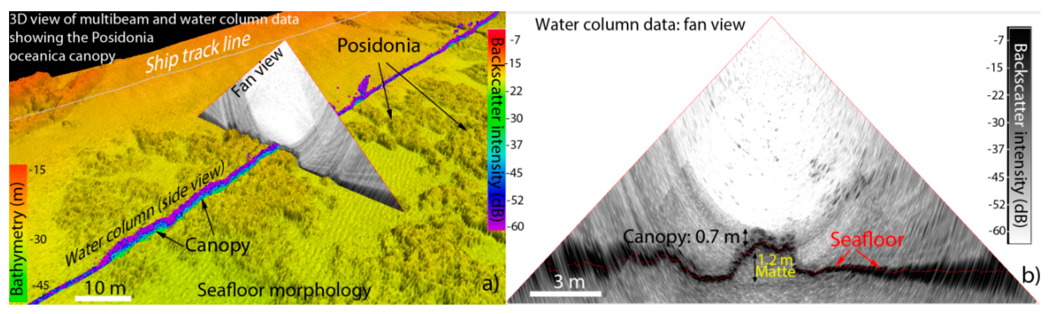
1.3. Application of Multibeam Systems in Seagrass Habitat Mapping

Side Scan Sonar (SSS) and Single-Beam Echo-Sounder (SBES), were considered as the most common acoustic methods for seafloor mapping and analysis [18,19,20,21]. More recently (i.e., a few decades ago) other techniques such as the Multibeam Echo-Sounder (MBES), allowed the acquisition of higher resolution bathymetry and backscatter data especially for seagrass meadows [22,23,24,25,26,27,28,29].

Bathymetry and backscatter data and their derived products (such as Slope, Aspect, Curvature and Terrain Ruggedness maps) can play a pivotal role in providing useful information for managing the world’s coasts and oceans [30]: seabed mapping with high-resolution MBES provides bathymetric profiles that can be visualized as a high-resolution Digital Elevation Models (DEMs) along with acoustic backscatter intensity from the seafloor and, more recently, from the water column [31,32,33,34] (Figure 1). Moreover, for seagrass meadow mapping, the MBES technique provides a three-dimensional reconstruction of the seafloor in shallow waters (from about 50 m to 10 m of depth) whereas optical (multispectral satellites images), methods are unable to provide detailed maps after 15–25 m in depth. Indeed, it delivers a precise and accurate bathymetric data for 3D reconstruction of seafloor morphologies (e.g., seagrass matte), by highlighting the presence of canopies of P. oceanica meadows (Figure 2).

However, the MBES surveys are limited in very shallow water areas especially at a 5 m depth where vessel navigation might be difficult and dangerous and the swath coverage is very limited (generally 3–4 times the depth of the seabed) and, hence, might significantly increase the surveying time and its costs.

1.4. Application of Unmanned Aerial Vehicles (UAVs) and Autonomous Surface Vehicles (ASVs) Systems in Seagrass Habitat Mapping

Marine observation techniques are usually divided into two major categories: (1) remotely acquired data and (2) field measurements that are required for validation. The first category includes satellite and aerial images, while the second includes techniques of ground-truth sampling like underwater images, videos, underwater photogrammetry, in situ measurements and sampling procedures. For seagrass habitat assessment, very fine resolution Unmanned Aerial Vehicle (UAV) imagery has been effective for density coverage mapping and for detecting changes in small patches and landscape features; these assessments would not have been possible with satellite or aerial photography [10,35,36,37,38]. However, the application of UAVs for mapping and monitoring of seagrass habitats has been limited by the optical characteristic of the water (e.g., turbidity), and the environmental conditions (e.g., solar elevation angle, cloud cover and wind speed) during image acquisition [39]. As such, most research has been confined to clear shallow tropical waters [40,41] or small subsets of exposed intertidal seagrass beds in temperate regions [36,37]. When it comes to Autonomous Surface Vehicles (ASVs), they are considered promising approaches in the marine science community. An immediate advantage is related to the collection of ground-truth data (optic and acoustic) with single-beam echosounders and images from underwater photogrammetry cameras, which ensures very high accuracy in very shallow waters [9,42,43]. This approach could represent, in the future, a replacement of diver seagrass investigations (i.e., snorkeling or scuba diving [11]) especially during either impractical or dangerous, field campaigns.

1.5. OBIA Classification Algorithms in Seagrass Habitat Mapping

Object-based image analysis (OBIA) is an advanced classification method that incorporates spectral, weight, color, texture, shape and contextual information to identify thematic classes in optical and acoustic data-derived images. The first step of OBIA classification is to perform a multiresolution segmentation of the image to identify homogeneous objects (note: the term “object” in this case stands for a contiguous group of spatial data such as pixels in a bathymetric grid). The segmentation process is based on predefined parameters such as compactness, shape and scale, derived from real-world knowledge of the characteristics to be identified and classified. For machine learning-based mapping, several algorithms have been developed to improve either the classification from satellite imagery or seagrass prediction from environmental parameters [44,45]. In a second step, the object-based classification uses machine learning algorithms such as Support Vector Machine (SVM), Random Tree (RT), Decision Tree (DT), Bayesian and k-Nearest Neighbor (k-NN) that have been further refined and are accessible on a variety of data analysis software. Seafloor mapping based on multibeam bathymetry and backscatter data using Object-based Image Analysis has been recently carried out by Janowski [46,47]. The authors found that OBIA-based approaches led to a doubling of the overall accuracy and Kappa measures, from 42% and 0.24–0.27, to 86% and 0.81. Some studies [45,48,49] already employ the OBIA technique for benthic habitat mapping and automatic classification analysis of reefs and seabed through the use the acoustic data of MBES or SSS has been described in several scientific works [47,50]. The OBIA technique applied to map coral reefs has successfully shown improved performance across different spatial scales [51,52,53,54]. Moreover, the OBIA technique is particularly suited for the analysis of very high resolution (VHR) images such as QuickBird or WorldView-2, where the increased heterogeneity of submeter pixels would otherwise confuse pixel-based classifications yielding to an undesired “salt and pepper effect”. Finally, in the study performed by Roelfsema et al. [55], the OBIA semiautomated approach proved to be very effective in extracting seagrass species and cover maps through the analysis of satellite images [56]. The UAV images and OBIA classifications have also been used together for the mapping of seagrass habitats [37,39,40,57].

2. Materials and Methods

In this work, an integrated approach has been followed for the detection and mapping of seagrass. In particular, multispectral images from satellite, aerial and underwater digital images from UAV/ASV, Underwater Towed Video Camera Systems (UTCS) and acoustic data from underwater sonar technology have been used to map the seagrass meadows and monitor their extent and condition (Figure 2).

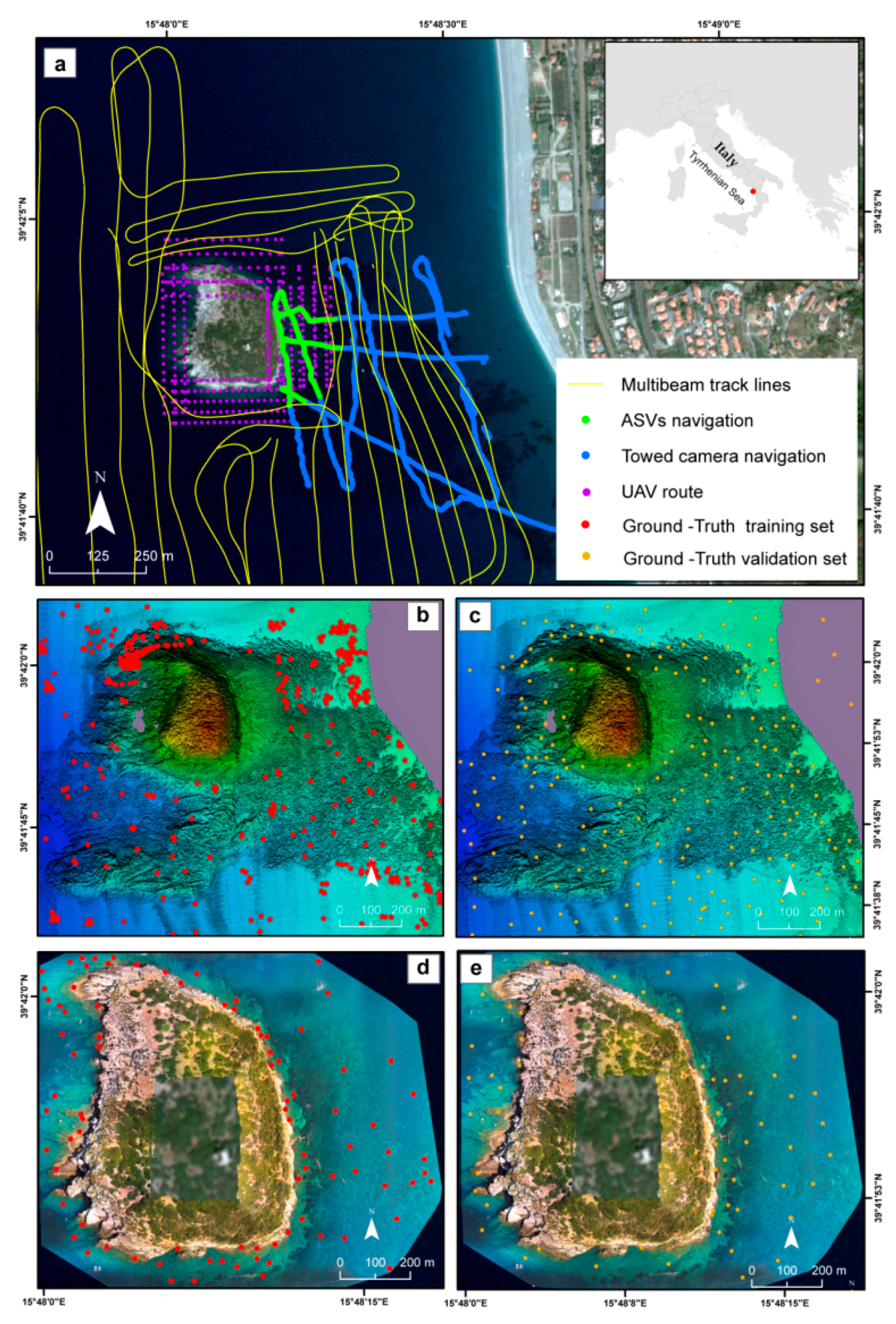
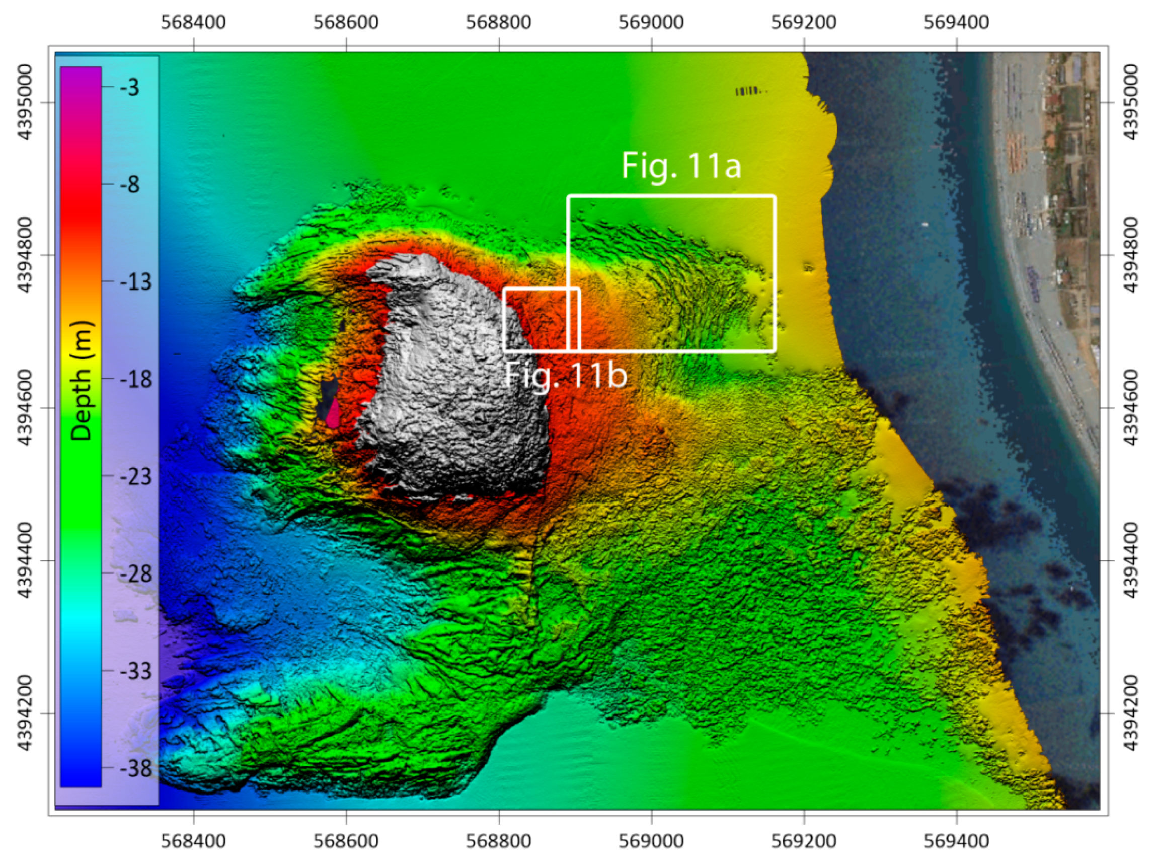
2.1. Study Sites and Geomorphological Characterization

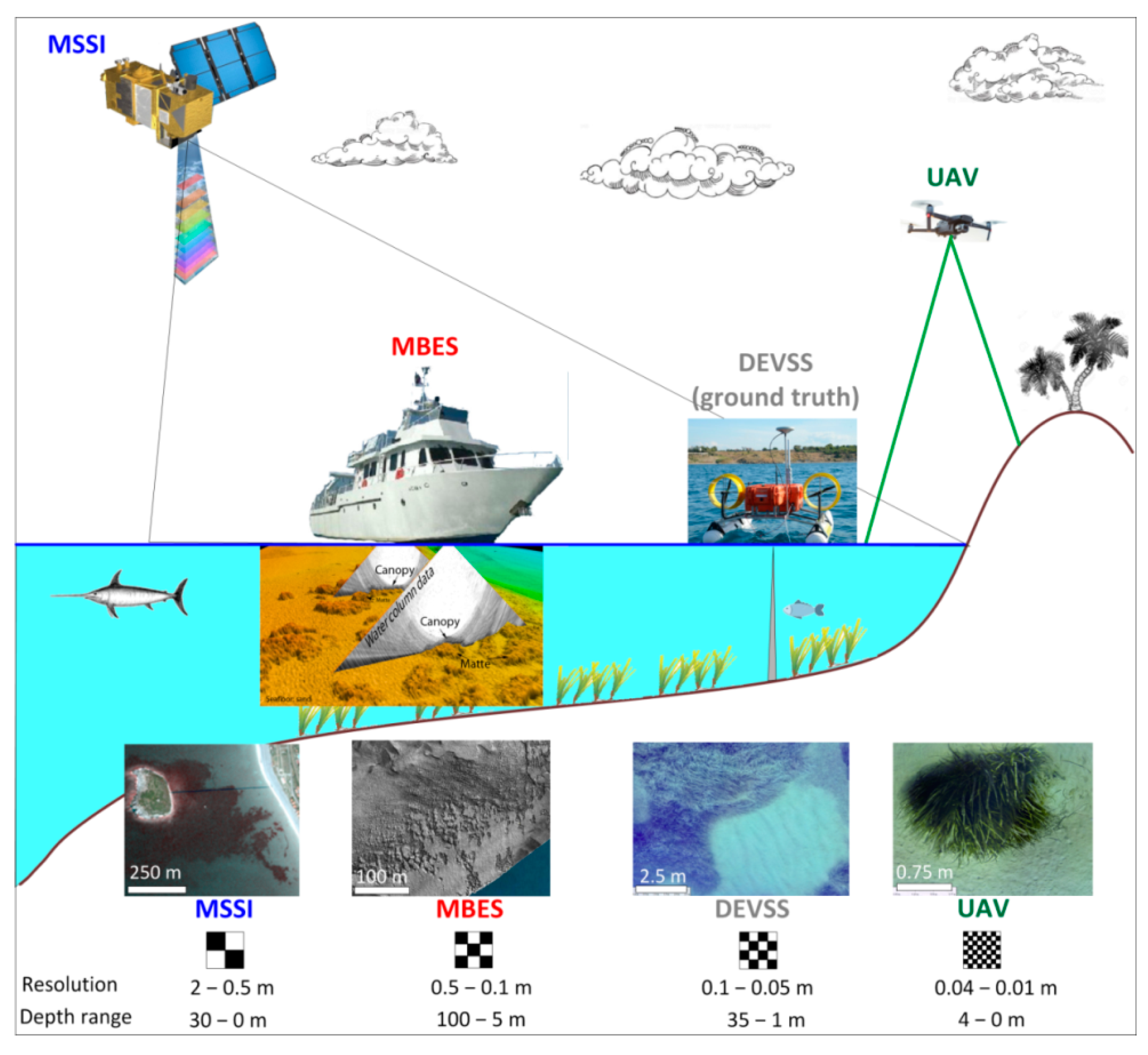
Fieldwork was carried out at Cirella Island, a Site of Community Importance in the Southern Tyrrhenian Sea (Lat 39°41′54.93″ N-Long 15°48′8.01″ E). Four kinds of surveys in 2018 and 2019 were carried out (Multibeam, UAV and Development Vehicle for Scientific Survey (DEVSS) and UTCS).

Cirella Island is located on the continental shelf at a distance of 600 m from the coast and 2.5 km from the shelf break (Figure 3). The island is composed of an emerged portion of about 0.07 km² and has a greater submerged portion of about 0.3 km²; both portions belong to a carbonate unit of limestone rocks from the Cretaceous [58]. The deeper seabed morphologies (from about 27 m to 41 m water depth) around Cirella Island are characterized by semiflat bottom with a low gradient of about 1–1.5° toward the shelf break (Figure 3a), while in shallow water the morphologies are quite rugged with a local gradient up to 70°. These morphologies are produced by rocky outcrops and by an extensive matte of P.oceanica.

P. oceanica is located both on sediment, represented mainly by sand, and on rocky outcrops. Overall, the coverage of P. oceanica is about 0.54 km² of which about 65% is located on rocky outcrops. The matte height is quite variable due to the rocky outcrop (maximum height: 1.5 m).

Around Cirella Island, the depth and distribution of P. oceanica is uneven. On the western side, it is located from a depth of 15 m while on the eastern side it is located from a depth of 3 m. These depths reflect the prevailing direction of the waves. Indeed, most of the waves come from the W and SW sectors (caused by Ponente and Sirocco winds, respectively, as shown in the elaboration of the the directional wave analyzed from NOAA database from 1979 to 2009). This suggests that their effect in shallow water is more relevant in the western sector of the study area which is exposed to both predominant wave directions.

2.2. Remote Sensing

The Pléiades satellite image acquired on 28 September 2016 was used for the study area. The Pléiades image was supplied with 4 spectral bands and 2 m of spatial resolution and was already orthorectified with pixel values in reflectance [59] (Figure 4a). The image was initially rectified using the Dark Object Subtraction (DOS) technique, with the aim of removing the disturbance related to the return flow of the atmosphere that separates the marine surface from the transported sensor aboard the satellite (Figure 4b).

The second processing performed a correction to compensate for the effects of light intensity attenuation as depth increases. This correction was made using the procedure proposed by [60] and by identifying and choosing homogeneous sandy bottoms at different depths. The aim was to identify, through appropriate regressions, the coefficients that allow correlating the reflectance values of the bottom pixels to the depth (Figure 4c).

The water column correction was carried out with the ERDAS IMAGINE software via the Spatial Modeler tool [61].

The bands of the Pléiades satellite image, used to obtain the water correction coefficients, are blue, green and red: in this specific case, three bands originated from the blue–green, blue–red and green–red pairs have been obtained from image processing. The three resulting bands were then combined to create a new color image that was considered more appropriate for the classification phase (compared to the unprocessed original image).

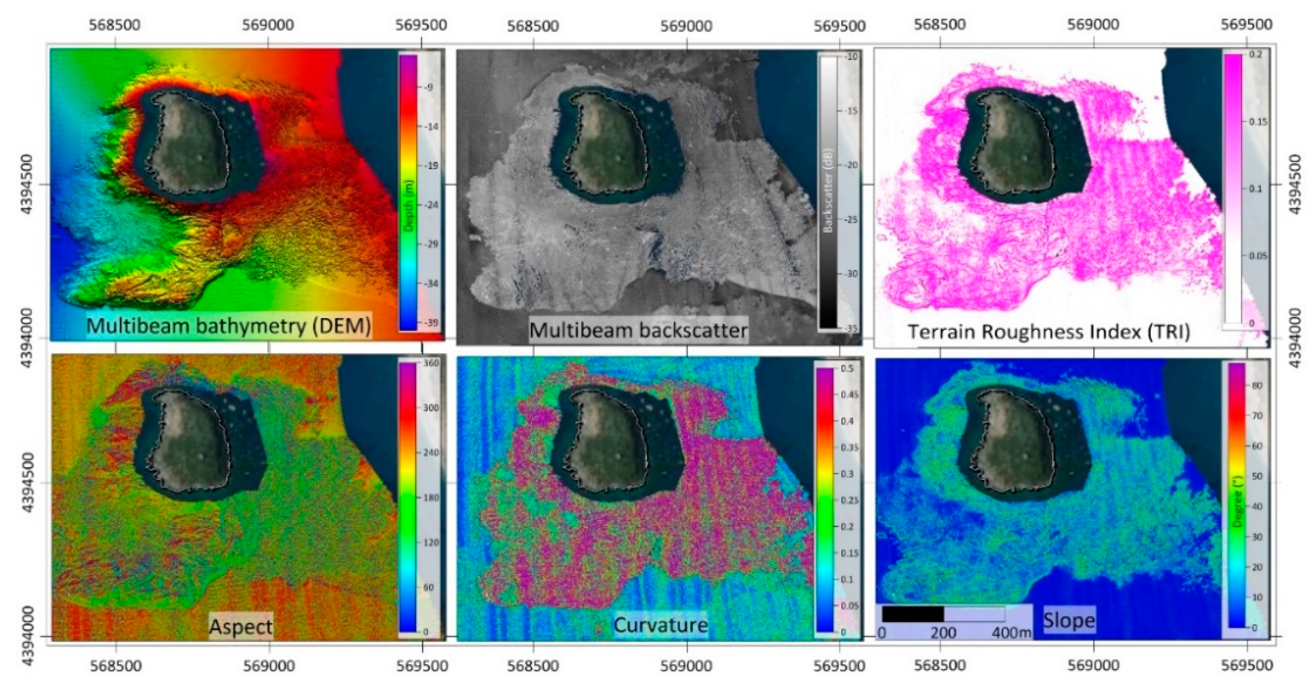
2.3. Multibeam Bathymetry

During 2018, in the SIC CARLIT project, high-resolution multibeam survey campaigns (bathymetry, backscatter and water column data), were performed in the Tyrrhenian sea (Figure 3). During this project, 535 nautical miles of multibeam bathymetry data in shallow water, covering 81 km² of the seafloor, were collected. However, the study area of Cirella Island described in this work was examined in just one day. The multibeam survey was carried out in September 2018 collecting data between 10 m and 40 m water depth with a Kongsberg EM2040 Multibeam Echo-Sounder System installed on “Astrea”, a 24 m long boat with a 3 m draft. The multibeam was set to use the equidistant mode with a frequency of 300 kHz and 256 beams per swath. A positioning system was installed: a Kongsberg Seapath 300 with the correction of a Fugro HP Differential Global Positioning System (horizontal accuracy: 0.2 m). A Kongsberg Seatex IMU (MRU 5) Motion Reference Unit recorded the attitude and rotation about the three orthogonal axes centered on the vehicle’s center of gravity (pitch, roll, heave and yaw movements). A Valeport mini sound velocity sensor (SVS), mounted in proximity to the transducers, measured continuously the sound velocity for the forming beam. Three sound velocity profiles were collected with a Valeport sound velocity profiler. Data were logged, displayed and checked in real-time with the Kongsberg SIS software (Seafloor Information System). Bathymetric multibeam data were processed using Caris HIPS and SIPS hydrographic software. The processing workflow consisted of a patch test and in the application of statistical and geometrical filters to remove coherent/incoherent noise [27,34]. Since the investigated area is a microtidal environment, particular attention was given to tidal corrections to make sure that the DEMs were corrected. The local hydrometric level was related to the permanent tide station of Palinuro, belonging to the National Tide gauge Network (http://www.mareografico.it). The backscatter intensity (BS) maps were created by using Caris HIPS and SIPS hydrographic software after applying the Angle Varying Gain (AVG) beam pattern correction to remove the angular dependence artifacts from the seabed backscatter. The soundings profiles were merged and gridded for the generation of DEMs at 0.3 m cell size resolution and the backscatter intensity map at 0.2 m cell size resolution. All data (DEMs, backscatter intensity map, UAV data and multispectral images), were merged through a GIS software (i.e., Global Mapper 20.0) that allowed to control the overlapping datasets positioning [62]. Furthermore, about 717 control points were used to validate, by direct observation, the Multibeam morphology, the ground-truth reference data for training, and the classification algorithm,

Table 1. Number of ground-truth data derived by the acoustic data MBES, and collected through the Underwater Towed Camera Systems (UTCs), ASVs DEVSS and UAV.

Class	MBES	UTCS	ASV	UAV
P. oceanica (P)	214	41	26	13
Rock (R)	95	\	6	50
Mobile Fine sediment (FS)	197	13	\	\
Coarse sediment (CS)	211	5	\	\
Cystoseira (Cy)	\	\	\	49
Total	717	59	32	112

.

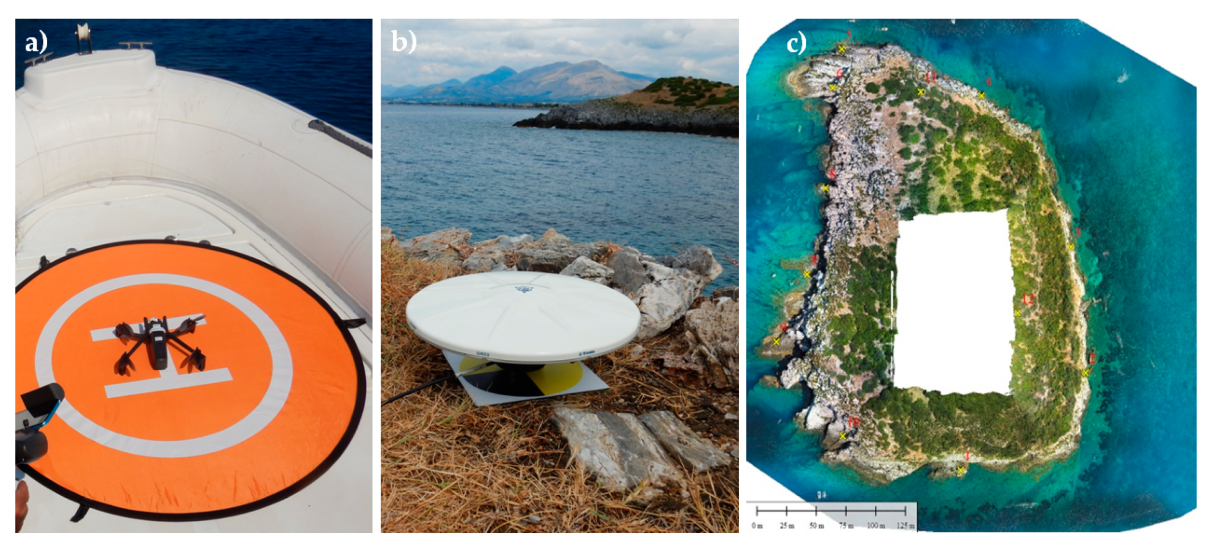
2.4. UAV Survey and Processing for Digital Terrain and Marine Model Generation

The images were collected across Cirella Island in July 2019 via a Parrot Anafi Work UAV. This model has an onboard camera with a 1/2.4-inch CMOS sensor which captures 21-megapixel images (.jpeg format) and an f/2.4 lens with an 84° field of view. Automated flights were carried out with the Pix4D Capture free drone flight planning mobile application with an 80% overlap on both axes, and a flight altitude that ranged between 60–75 m depending on the total size of the surveyed site. In total, 4 photogrammetric flights were performed in order to cover the north/south and east/west side of the island. A total of 360 frames were captured during a continuous flight (Figure 5). The surveyed images were processed with Pix4D Mapper software [63] by using 11 ground control points located around the island between 0 and 10 m altitude. The mosaic image and the DEM were processed at 0.02 m and 0.3 m resolution respectively. In particular, 112 frames were used to collect, by UAV direct observation, the ground-truth reference data for training and validating the classification algorithm, Table 1.

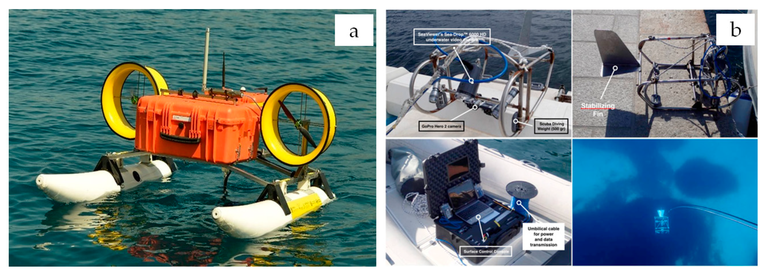
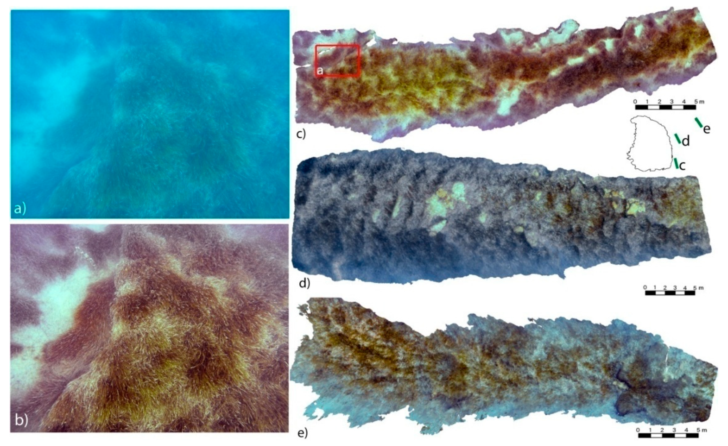
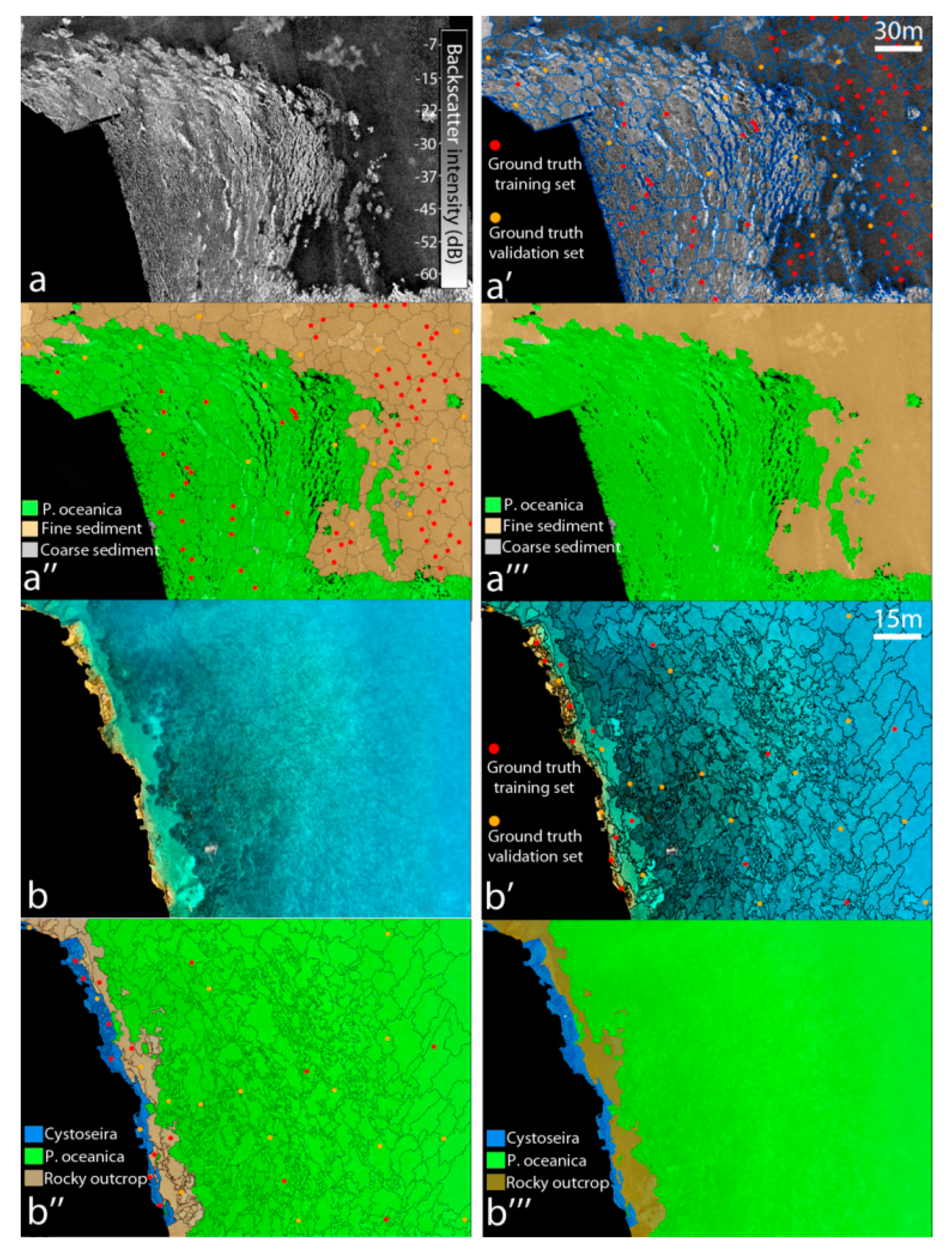
2.5. Image Ground-Truth Data

The ASV robotic platform DEVSS (DEvelopment Vehicle for Scientific Survey) developed by the 3D Research private research company [64] and the Underwater Towed Camera Systems (UTCS) were used, in the very shallow water area, to collect the ground-truth reference data for training and validating the classification algorithm, Table 1 [65]. The ASVs was equipped with a GoPro Hero 4 Black model, which is a consumer-brand high-definition sports camera with a 12 MP HD CMOS sensor, 1/2.5″ size [64]. The GoPro Hero 4 Black records at different video and photo resolutions and Field-Of-View (FOV). In this work, we used the camera (set in time-lapse mode) with 12 MP widescreen 1080 p and a FOV of 108°. The camera was positioned face-down in order to obtain vertical images at the same height from the bottom. In the shallow water area, time-lapse photos were recorded by using: an UTCs Platform, equipped with a caudal fin in order to reduce pitch and roll movements and stabilize video acquisition, a SeaViewer’s Sea-Drop™ 6000 high-definition underwater video camera, with a surface console and two GoPro Hero 3+ cameras (Figure 6b), with a 12 MP HD CMOS sensor f 2.8–170° [66] (Figure 6b).

The combined sampling of acoustic and optical data was carried out in the shallow water coastal area (depth < 10 m) that surrounds Cirella Island. In order to acquire overlapping pictures, ensuring about 75% of shared coverage between two consecutive photos, a speed of about 1 knot/h was maintained. A total of about 2500 georeferenced images were collected. Before performing the 3D processing, an underwater image enhancement technique [67] was performed to minimize the effect of the water column on the underwater images. After the image enhancement step, a Structure-from-motion (SfM) 3D reconstruction was performed using the commercial software Agisoft Metashape Pro and Pix4D mapper [68]. The average root-mean-square error (RMSE) achieved at this step was 0.022 m for GPS coordinates. Finally, a Multiview Stereo (MVS) algorithm was used by the Metashape software to produce a dense 3D point cloud from the refined intrinsic orientation and ground-referenced camera exterior orientation (Figure 7). In particular, in the very shallow water area, 32 sampling areas were acquired with Autonomous Surface Vehicle DEVSS and 59 sampling areas were acquired with UTCS in the shallow water area, Table 1 [64]. The 3D reconstructions generated by DEVSS and UTCS were used in order to: (a) interpret the bathymetric DEM and backscatter and (b) identify further ground-truth data.

In general, all the ground-truth data used in this work were carefully checked for possible overlaps between the training and validation samples. The minimum distance, calculated between any training and validation samples, was about 25 m and this affects only 10% of the total dataset.

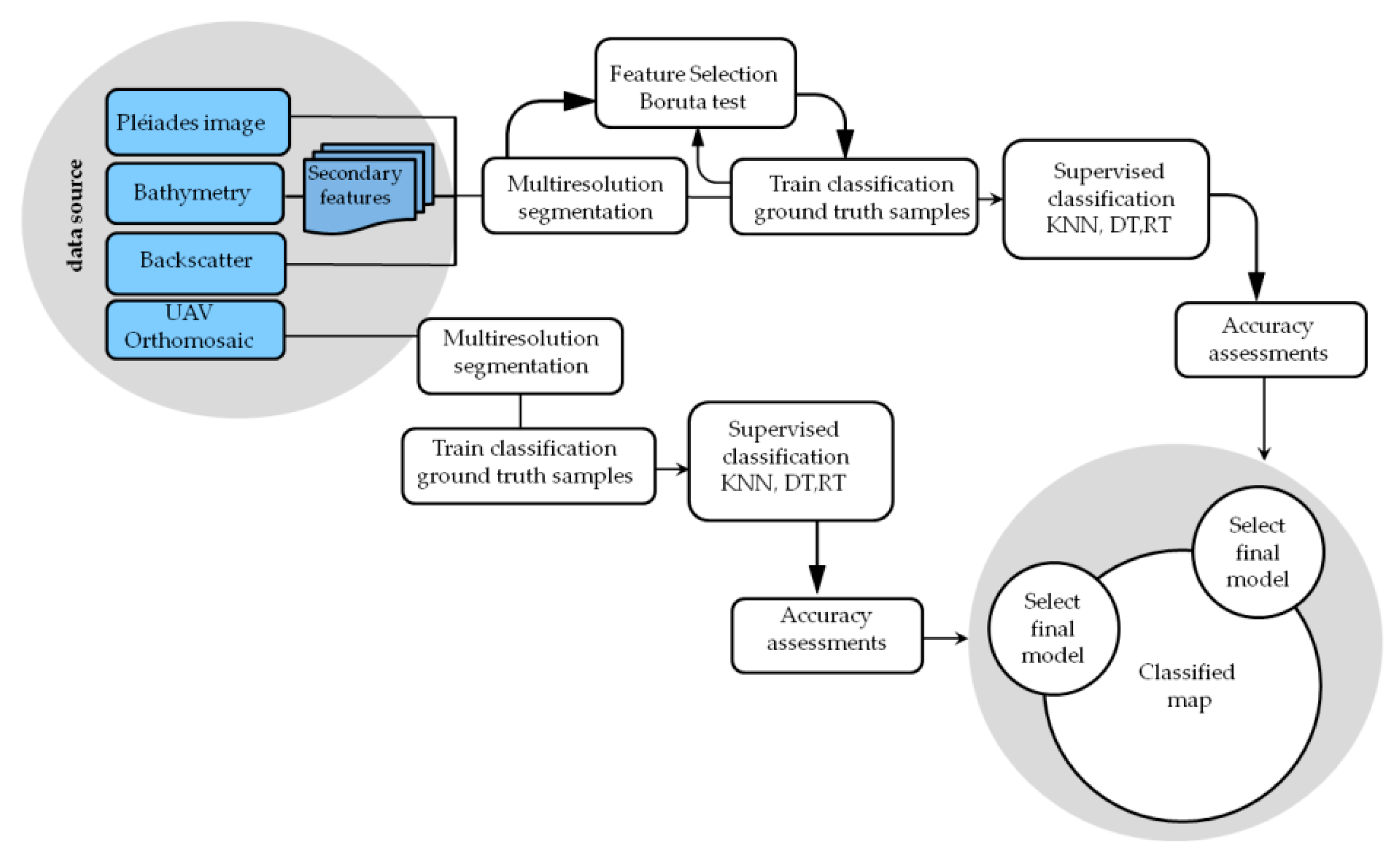
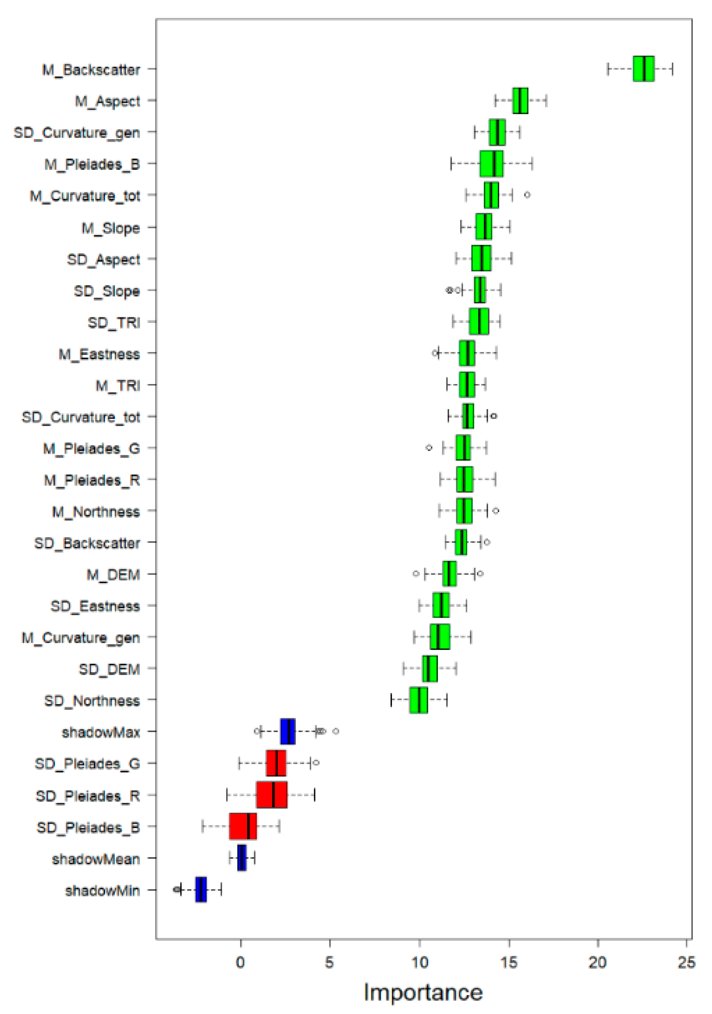
2.6. OBIA Segmentation and Classification

All collected data, i.e., DEMs, backscatter intensity map, UAV data and multispectral images data, were processed in the OBIA process [69] by eCognition Essentials 1.3. software, using a classification algorithm [70] (Figure 8). The Multibeam bathymetry data were converted into secondary features: Slope, Northness, Eastness, Curvature and Terrain Roughness Index (TRI) using the Morphometry Tool in SAGA (SAGA (System for Automated Geoscientific Analyses) Version) [71] as shown in (

Table 2. Multidata source variable and list of extracted secondary features of the bathymetric and backscatter data.

Source	Features	Resolution	Software	Area
Multibeam EM2040	Backscatter/Bathymetry	0.3 m	Caris HIPS and SIPS	shallow
Bathymetry	Curvature General	0.5 m	SAGA-GIS	shallow
Bathymetry	Curvature Total	0.5 m	SAGA-GIS	shallow
Bathymetry	Slope	0.5 m	SAGA-GIS	shallow
Bathymetry	Aspect	0.5 m	SAGA-GIS	shallow
Bathymetry	Northness	0.5 m	SAGA-GIS	shallow
Bathymetry	Eastness	0.5 m	SAGA-GIS	shallow
Bathymetry	Terrain Ruggedness Index (TRI)	0.5 m	SAGA-GIS	shallow
Pléiades	Satellite image	2 m	ERDAS IMAGINE	shallow
UTCS	Image Truth data	0.001 m	AGISOFT METASHAPE	shallow
Parrot Anafi Work	Orthophoto	0.02 m	PIX4D Mapper	very shallow
ASVs (DEVSS)	Image Truth data	0.001 m	AGISOFT METASHAPE	very shallow

and Figure 9).

The multiresolution segmentation algorithm, performed by the eCognition Essential software, was used to identify homogeneous objects. The process of multiresolution segmentation was carried out by considering the following parameters: Scale Factor, Shape, Smoothness and Compactness. In shallow water, the multiresolution segmentation algorithm was used to generate objects with similar information by using only the backscatter intensity and TRI features. The bathymetry, Slope, Aspect and Curvature features were excluded from this first segmentation procedure. The multiresolution segmentation algorithm was used to generate objects with similar information by using only the most important features selected. This decision was taken since the use of all features (primary and secondary) had created an excessive disturbance effect and the segmentation results were not adapted to the real shapes of the objects. In order to identify and remove nonimportant features from all the input layers, a feature selection algorithm (i.e., the R package Boruta algorithm) was used to assess their relevance in determining the thematic classes. The Boruta algorithm is built on a “random” forest classification algorithm. With the wrapper algorithm, present in the Boruta package, we selected all the relevant features by comparing the importance of the original attributes with the importance reached in a random way, estimated using permutations (i.e., shadows). Only the features whose importance was higher than those of the randomized features were considered important [72]. The Boruta algorithm result gave a list of attributes according to their importance, separating them into “confirmed” or “rejected” features. The features without decision at the end of the analysis were classified as “provisional”. In the following classification step, we used the 10 most important attributes considered as “confirmed” by the Boruta algorithm. Therefore, the Boruta test allows identification of the most important and nonredundant features to train a model improving the learning process timing and accuracy of the final classification map (Figure 8). The orthophotos generated from UAV data surrounding the area around the Cirella Island (seabed depth from 0 to 12.5 m) were treated separately by the eCognition software due to the lack of data acquired from multibeam surveys in very shallow water. Therefore, two different projects within the eCognition Essential software were created. The first included all data acquired by multibeam in shallow water areas (8–30 m) and the second included only the orthophotos acquired by UAV in very shallow water areas (1–12.5 m; Table 1). We tested the performance of the three different supervised classification algorithms available in the eCognition Essential software: (k-NN), (RT) and (DT). The k-NN algorithm is a method for classifying objects by a majority ranking of its neighbors—with the object being assigned to the class most common among its k-Nearest neighbor. DT learning is a method commonly used in data mining where a series of decisions are made to segment the data into homogeneous subgroups through a tree system with branches. Random tree is a combination of tree predictors where each tree depends on the values of a random vector, sampled independently and with the same distribution for all trees in the forest [73]. All trees are trained with the same features but on different training sets, which are generated from the original training set. It aggregates the ranks from different decision trees in order to assign the final class of the test object. The ground-truth data acquired with the direct interpretation of multibeam data, by means of the ASV DEVSS (both images and 3D point clouds) and the UTCS platform were used to assign specific class values to the segmented objects. In the sampled area, five different classes were identified: Fine sediment-FS, Coarse sediment-CS, Rock-R, P. oceanica meadows-P and Cystoseira-Cy. Some samples were identified through other techniques in order to have homogeneous ground-truth data coverage. Along the perimeter of the island, in the very shallow water areas, ground-truth data were taken directly via visual identification during UAV survey, while for deeper areas that could not be reached by the ASV DEVSS, some ground-truth data were selected based on the study of multibeam bathymetry, backscatter and water column data acquired during the multibeam survey and by direct observation with the UTCS platform. Overall, 920 ground-truth data were used in this study and divided into two different groups (Training set and Validation set): one to perform the training step and the second to evaluate the classification accuracy and Kappa coefficients [74,75,76] (

Table 3. Main thematic classes of seabed and number of ground-truth data collected through the ASV DEVVS, UTCS, UAVs and derived by the acoustic data.

	Shallow Water		Very Shallow Water
Class	Training Set	Validation Set	Training Set	Validation Set
P. oceanica (P)	123	122	23	26
Rock (R)	80	15	35	21
Fine sediment (FS)	207	170	\	\
Coarse sediment (CS)	44	5	\	\
Cystoseira (Cy)	\	\	31	18
Total	454	312	89	65

and Figure 3).

3. Results

Multibeam and photogrammetric (UAV) DEMs were merged via Global Mapper software using the acoustic data and point cloud raw data respectively. The cloud points obtained by Pix4D software were georeferenced by comparing the position of the Ground Control Points detected along the coastline and on the island, while the bathymetric data collected with multibeam were used in order to correct the altitude in the marine area. This operation was carried out through the tools for Quality Control of LiDAR point cloud data LiDAR module of the Global Mapper software allowing comparison and/or 3D correction of the height of point cloud data to known control points, and to report statistics about subsets of points.

The acoustic profiles and point clouds were gridded (0.3 m) generating an integrated digital land and sea model, overall the merged soundings and cloud points highlighted a vertical subdecimetrical accuracy, see Figure 10.

In the shallow water areas, the most relevant results were obtained by using the following multiresolution segmentation parameters: scale segmentation 20; Shape 0.1, compactness 0.5 and scale slider min. value 10, scale slider max value 100. These parameters were selected after several tests carried out with different settings comparing the segmentation objects created by the algorithm with those of real morphology. Figure 10 shows the two Areas of Interest (AOI) from which we have extracted the two examples of segmentation and classification processes. The results are shown in Figure 11.

The acquired ground-truth data were used to assign specific class values to determine segmented objects (Figure 11).

All statistical information about the features (primary and secondary), associated with the objects classified from 766 ground-truth data (training and validation set) were extracted from eCognition Essential software and analyzed with the Boruta R package (version 6.0.0) in order to assess their importance in the assignment of the corresponding class (Figure 12) [77]. The classification tests performed with a higher than 10 number of attributes used in the training phase did not significantly increase the accuracy of the classification. The most relevant features emerging from the Boruta test, are the following in order of importance: the mean backscatter intensity, the mean Aspect, the general Curvature standard deviation, mean Pléiades Blu band, the mean of Total Curvature, the mean of Slope, the Aspect standard deviation, the Slope standard deviation, TRI standard deviation; the mean of Eastness. Figure 12 shows the results of the Boruta test.

The comparison between the different classification algorithms available in the eCognition Essential software: (k-NN), (RT) and (DT) was performed considering three levels of data combination: (A) Pléiades image; (B) Pléiades image combination with backscatter and bathymetry data; (C) Pléiades image combination with backscatter, bathymetry data and secondary features, (

Table 4. Accuracy assessment for the DT, k-NN and RT supervised classification algorithm (shallow water area) for 3 different combinations: (A) Pléiades image; (B) Pléiades image-Backscatter-Bathymetry; (C) Pléiades image-Backscatter-Bathymetry-Secondary features.

Combinations (Data Source)		Decision Tree (DT)		Random Tree (RT)		k-NN
A Pléiades image		Overall accuracy: 67.83% K: 0.48		Overall accuracy: 66.78% K: 0.47		Overall accuracy: 71.33% K: 0.48
	Class	User’s accuracy	Producer’s accuracy	User’s accuracy	Producer’s accuracy	User’s accuracy	Producer’s accuracy
	(P)	75.36%	85.25%	72.67%	89.34%	70.31%	73.77%
	(R)	83.33%	33.33%	83.33%	33.33%	100.00%	33.33%
	(FS)	84.21%	55.56%	87.80%	50.00%	75.35%	74.31%
	(CS)	10.64%	100.00%	10.42%	100.00%	18.18%	40.00%
B Pléiades-Backscatter Bathymetry		Overall accuracy: 83.61% K: 0.73		Overall accuracy: 91.80% K: 0.85		Overall accuracy: 82.38% K: 0.69
	Class	User’s accuracy	Producer’s accuracy	User’s accuracy	Producer’s accuracy	User’s accuracy	Producer’s accuracy
	(P)	95.45%	77.78%	96.97%	88.89%	90.22%	76.85%
	(R)	28.57%	80.00%	42.11%	80.00%	42.11%	80.00%
	(FS)	100.00%	88.43%	100.00%	95.04%	89.92%	88.43%
	(CS)	23.81%	100.00%	45.45%	100.00%	21.43%	60.00%
C Pléiades-Backscatter Bathymetry Secondary features		Overall accuracy: 88.57% K: 0.80		Overall accuracy: 99.63% K: 0.99		Overall accuracy: 86.94% K: 0.77
	Class	User’s accuracy	Producer’s accuracy	User’s accuracy	Producer’s accuracy	User’s accuracy	Producer’s accuracy
	(P)	94.95%	86.24%	100.00%	99.07%	94.95%	86.24%
	(R)	43.75%	70.00%	100.00%	100.00%	43.75%	70.00%
	(FS)	94.74%	89.26%	99.31%	100.00%	94.74%	89.26%
	(CS)	25.00%	80.00%	100.00%	100.00%	25.00%	80.00%

C). The best classification performance was obtained with the multilayer combination (Table 4C). The algorithm (RT) generally provided the best overall accuracy results in two levels of data combinations (B and C). In particular, the algorithm (RT), compared to the k-NN and RT algorithms, showed an overall accuracy of 99.63% and the Kappa coefficient 0.99, the Producer’s accuracy and User’s accuracy values with a low gap between them (Table 4C). The k-NN algorithm returned overall accuracy values of 86.94% and the Kappa coefficient 0,80, while the DT learning, showed an overall accuracy of 88.57% and the Kappa coefficient 0.77 (Table 4C). The k-NN algorithm did not show the best response in terms of classification (Table 4), whereas the DT learning showed an overall accuracy always lower than RT (Table 4). As shown in Table 4, in the RT all classes had a relatively consistent accuracy, as shown by the small differences between User’s and Producer’s Accuracy for each thematic map class. Results from the DT approach showed the divergence of the Producer’s and User’s accuracy increases considerably (Table 4).

In the very shallow water area, the same workflow was performed to generate the classified habitat map (Figure 8). The UAV orthophoto was imported via the eCognition software and a multiresolution segmentation algorithm in order to identify objects. The most relevant segmentation results were obtained by using the following parameter settings: scale 300; Shape 0.1, compactness 0.5 and scale slider min. value: 50, scale slider max. value: 600 (Figure 11). These parameters were selected after several tests carried out with different settings comparing the shapes created by the algorithm with those of the real morphologies of the seabed.

A greater scale was used for the orthophotos due to the higher image resolution (0.03 m). Data available for the OBIA classification derived only from the RGB orthophoto image, therefore the Boruta algorithm was not used. In the very shallow water area, 3 different classes were identified (Cystoseira (Cy), Rock (R), P. oceanica meadows (P); Table 2). The supervised classification algorithms (k-NN, RT and DT) were tested, but in this case, the best classification result in terms of accuracy was obtained when using the k-NN algorithm, with an overall accuracy equal to 95.24% and Kappa coefficient 0.92 (

Table 5. Accuracy assessment for the DT, k-Nearest Neighbors’ algorithm (k-NN) and RT supervised classification algorithms (very shallow water area).

	Decision Tree (DT)		Random Tree (RT)		k-NN
	Overall Accuracy: 74.6%		Overall Accuracy: 77.78%		Overall Accuracy: 95.24%
	K: 0.61		K: 0.65		K: 0.92
Class	User’s accuracy	Producer’s accuracy	User’s accuracy	Producer’s accuracy	User’s accuracy	Producer’s accuracy
(P)	71%	65.38%	66.70%	100%	100.00%	100.00%
(R)	62.50%	75%	88%	35.00%	87.00%	100.00%
(Cy)	100.00%	88.24%	100%	94.12%	100.00%	82%

). With regard to the k-NN classification algorithm, all classes (Cystoseira, Rock and P. oceanica) showed small differences between the Producer’s and User’s accuracy values (Table 5).

The two best-classified habitat maps (very shallow and shallow maps) selected on the basis of accuracy were merged into one very high-resolution classified map (Figure 13 and Figure 14).

More specifically, about 51 hectares of P.oceanica were mapped, while 119 hectares and 1.70 hectares were, respectively, identified for the Fine and Coarse sediment, and 0.45 hectares for Cystoseira.

4. Discussion

The main objective of this work was to perform benthic habitat mapping by using several data acquisition platforms and OBIA algorithms and to develop a high-resolution seagrass mapping digital elevation model. OBIA algorithms are now stable and powerful approaches to use for classifying benthic habitats and to produce accurate maps [78,79,80,81,82]. In this work, an integrated methodological approach has been followed for multisensor data fusion (acoustic and optical) with different degrees of resolution. This approach might be useful, if necessary, for mapping the P. oceanica meadows, but also seabed geomorphological features and furthermore, to estimate the carbon sequestration and storage of the seagrass ecosystem [83]. Generally, surveying techniques are used individually, and show several limitations such as spatial coverage in very shallow waters (e.g., Multibeam) or poor resolving capacity (e.g., satellite images) that might not allow a complete characterization of the spatial and temporal extent of P. oceanica meadows in deeper areas. Most benthic seagrass habitat mapping studies examine a single data source and quite a few attempts have been made to combine multiple data sources [84,85]. High spatial resolution satellite imagery (2 m or smaller) alone has proven to be unable to produce adequate accuracy for fine descriptive detailed maps [51] (a fact that is also confirmed by this study). High-resolution multispectral and hyperspectral imagery can be useful in discriminating habitat community size to a not-so-fine detail, but its moderate spatial resolution might limit its broader application especially as the depth of the seabed increases, and reflectance and radiance are absorbed [86]. The present study highlights how the OBIA classification did not provide a satisfactory result in terms of thematic accuracy by using only the Pléiades satellite images. Indeed, satellite images can be effective for the mapping of P. oceanica meadows, only in conditions of high water transparency and in the presence of excellent spatial and spectral resolution. However, the combination of acoustic bathymetric data (DEM and backscatter) combined with optical data (e.g., multispectral satellite) has proven to improve the final classification performance. The set of optical and bathymetric acoustic data combined with secondary features showed the best classification results and this has also been confirmed by other studies [14,35,87]. The present work, specific on high-resolution seagrass mapping, highlights how RT seems to be the OBIA algorithm with the best classification performance. Similar answers on RT have been highlighted also by Janowski [47] on the automatic classification of benthic habitats [78,80,81]. As far as the K-NN classifier is concerned, it has a lower case history of application in marine habitat mapping studies [79], and in general, the performances of the K-NN classifier were almost always moderate or fair. The RT algorithm in this study proved to be very effective in generating accurate classification, thus showing fair performance. Instead, the DT classification algorithm has always shown the lowest accuracy. The classification of the orthophoto produced with the UAV showed instead the best accuracy with the k-NN algorithm, which, although not much used for marine habitat mapping, has nevertheless obtained an excellent result compared to the DT and RT algorithms. The OBIA object classification, as highlighted in existing literature [45], represents an effective tool to obtain robust thematic maps.

The Boruta feature selection algorithm showed promising results on seagrass habitat mapping [23,66]. The results confirmed the usefulness of applying this feature selection method in seagrass habitats mapping [47]. The multiresolution segmentation scale requires careful adjustment of the value and represents a very important setting for correct classification by OBIA and has a significant impact on the results of seagrass habitat classification [48]. Multiresolution segmentation represents a very important step in the whole process, so defining the wide range of parameters, first of all, the scale factor, the shape, the Smoothness and Compactness, is of paramount importance since they can determine the good progress of the classification. In this work, even if only five thematic classes have been used (Fine sediment (FS), Coarse sediment (CS), Rock (R) P. oceanica meadows (P) and Cystoseira (Cy), Figure 13), it has been necessary to increase the number of ground-truth data for training and validation in order to improve the answers of the classification algorithms. In order to obtain a relatively high number of ground-truth data, different sampling platforms have been integrated and used, such as acquisitions with ASV, UAV, UTCS and direct observation and interpretation of the backscatter and DEM data, obtained by the Multibeam acquisition (Figure 9). This integrated technique could be useful to reduce the time and costs for the acquisition of ground-truth data.

The accuracy of habitat classification might be affected by multiple factors, including habitat heterogeneity, bathymetry and water column attenuation [88]. This study highlights how the integration of satellite imagery with ultrahigh spatial resolution UAV aerial imagery and bathymetric acoustic data shows a good performance in habitat classification [24]. The integrated multisource technique represents, indeed, an improved solution to map benthic habitats with high degrees of spatial accuracy. Therefore the higher the quality and spatial resolution of the data the better the performance of the segmentation algorithm and resulting OBIA classification [45,83,88] and consequently the generation of thematic maps. A high-resolution seabed classification map has been obtained for producing high-quality habitat-classified maps (Multilayer data and UAVs data). Two maps (shallow and deep water classified area) have been selected based on an accuracy assessment (shallow and deep water classified area) and have been merged into a unique and complete habitat map (Figure 13 and Figure 14).

At this stage, in the shallow classification, the integration of Pléiades satellite image, bathymetric and backscatter data has shown that the contribution of the optical component of the satellite data alone did not confer any clear improvements in the classification procedure. Therefore, for future implementations of the method, the team will evaluate how the different types of satellite sensors, the different characteristics of satellite images, in terms of spatial and spectral resolution, can improve the results of the multilevel classification.

Finally, the adopted methodological approach has proven its ability to extract information of geomorphological data related to marine ecosystems from the coast to the deep areas, in a georeferenced 3D environment. This provides important geoinformation on the extension of the three-dimensional coverage (area extensions and volumes) of the benthic macrohabitats necessary for the analysis of data such as blue carbon.

5. Conclusions

The integration of different methodological techniques (Multibeam, UAV, DEVS, UTCS and multispectral image) represents a rapid and effective method for high-resolution seafloor and habitat mapping from the coastline to deeper water. The geophysical and optical techniques, if correctly processed, allow generation of high resolution integrated terrestrial and marine digital elevation models that can also be used for the analysis of the physical environment both in the geological context and in oceanographic modeling. Furthermore, these processed data can be used for time-lapse analysis aimed to verify seabed changes, such as, the loss of seagrass habitats, migration of sediments (erosional and depositional processes), as well as the anthropogenic impacts caused by fishing activities or leisure boating.

The processing carried out from the multisensor (optical–acoustic) data fusion has significantly improved the resolution of the mapping of the P. oceanica meadows mainly along the upper limit, especially in shallower areas where data acquisition, performed with orthophoto UAVs image, are more likely to be valid. The best results of the Object-based Image classification were achieved with combined processing of DEM bathymetry, backscatter, secondary data and optical satellite data. The worst and most inaccurate results of the Object-based classification were obtained when processing relied only on Pléiades satellite image.

Based on the increasing use of thematic maps for habitat and the current interest in using seagrass extension as a monitoring indicator, this digital cartographic method improves the quality (limits of benthic facies) of the final maps, returning high-resolution products with high spatial and thematic accuracy.

The integration of multiple acquisition methods (Satellite sensor, UAV, DEVS, UTCS and Multibeam) allows to map the full extension of the P. oceanica meadows starting from very shallow waters up to the lower limit; improves the performance of the cost-efficiency of the monitoring according to the quality response of every single sensor (acoustic and/or optical), reduces the monitoring execution time of the acoustic surveys with the Multibeam in very shallow water areas, which generally require higher costs and more time to perform the surveys. This mapping technique may represent, within the Marine Strategy Framework Directive (MFSD-2008/56/EC) and the EU Habitat Directive (92/43/CEE), a valid methodology to determine the habitat extend and condition of P. oceanica meadows and to quantify also the carbon sinks and capture rates of seagrass meadows.

References

1. Green, E.P.; Short, F.T.; Frederick, T. World Atlas of Seagrasses; University of California Press: Berkeley, CA, USA, 2003. [Google Scholar]
2. Den Hartog, C.; Kuo, J. Taxonomy and Biogeography of Seagrasses. In Seagrasses: Biology, Ecologyand Conservation; Springer: Dordrecht, The Netherlands, 2007; pp. 1–23. [Google Scholar] [CrossRef]
3. EEC. Council Directive 92/43/EEC of 21 May 1992 on the conservation of natural habitats and of wild fauna and flora. Off. J. Eur. Commun. 1992, 206, 7–50. [Google Scholar]
4. Serrano, O.; Kelleway, J.J.; Lovelock, C.; Lavery, P.S. Conservation of Blue Carbon Ecosystems for Climate Change Mitigation and Adaptation. In Coastal Wetlands, 2nd ed.; Elsevier: Amsterdam, The Netherlands; Oxford, UK; Cambridge, MA, USA, 2019; pp. 965–996. [Google Scholar] [CrossRef]
5. Orth, R.J.; Carruthers, T.J.B.; Dennison, W.C.; Duarte, C.M.; Fourqurean, J.W.; Heck, K.L.; Randall Hughes, A.; Kendrick, G.A.; Kenworthy, W.J.; Olyarnik, S.; et al. A global crisis for seagrass ecosystems. Bioscience 2006, 56, 987–996. [Google Scholar] [CrossRef] [Green Version]
6. Duarte, L.D.S.; Machado, R.E.; Hartz, S.M.; Pillar, V.D. What saplings can tell us about forest expansion over natural grasslands. J. Veg. Sci. 2006, 17, 799–808. [Google Scholar] [CrossRef]
7. Turner, S.J.; Hewitt, J.E.; Wilkinson, M.R.; Morrisey, D.J.; Thrush, S.F.; Cummings, V.J.; Funnell, G. Seagrass patches and landscapes: The influence of wind-wave dynamics and hierarchical arrangements of spatial structure on macrofaunal seagrass communities. Estuaries 1999, 22, 1016–1032. [Google Scholar] [CrossRef]
8. Lathrop, R.G.; Montesano, P.; Haag, S. A multi scale segmentation approach to mapping seagrass habitats using airborne digital camera imagery. Photogramm. Eng. Remote Sens. 2006, 72, 665–675. [Google Scholar] [CrossRef] [Green Version]
9. O’Neill, J.D.; Costa, M. Mapping eelgrass (Zostera marina) in the Gulf Islands National Park Reserve of Canada using high spatial resolution satellite and airborne imagery. Remote Sens. Environ. 2013, 133, 152–167. [Google Scholar] [CrossRef]
10. Hogrefe, K.; Ward, D.; Donnelly, T.; Dau, N. Establishing a baseline for regional scale monitoring of eelgrass (Zostera marina) habitat on the lower Alaska Peninsula. Remote Sens. 2014, 6, 12447–12477. [Google Scholar] [CrossRef] [Green Version]
11. Reshitnyk, L.; Robinson, C.L.K.; Dearden, P. Evaluation of WorldView-2 and acoustic remote sensing for mapping benthic habitats in temperate coastal Pacific waters. Remote Sens. Environ. 2014, 153, 7–23. [Google Scholar] [CrossRef]
12. Traganos, D.; Aggarwal, B.; Poursanidis, D.; Topouzelis, K.; Chrysoulakis, N.; Reinartz, P. Towards Global-Scale Seagrass Mapping and Monitoring Using Sentinel-2 on Google Earth Engine: The Case Study of the Aegean and Ionian Seas. Remote Sens. 2018, 10, 1227. [Google Scholar] [CrossRef] [Green Version]
13. Finkl, C.W.; Makowski, C. The Biophysical Cross-shore Classification System (BCCS): Defining Coastal Ecological Sequences with Catena Codification to Classify Cross-shore Successions Based on Interpretation of Satellite Imagery. J. Coast. Res. 2020, 36, 1–29. [Google Scholar] [CrossRef] [Green Version]
14. Hossain, M.S.; Bujang, J.S.; Zakaria, M.H.; Hashim, M. The application of remote sensing to seagrass ecosystems: An overview and future research prospects. Int. J. Remote Sens. 2015, 36, 61–114. [Google Scholar] [CrossRef]
15. Pham, T.D.; Yokoya, N.; Bui, D.T.; Yoshino, K.; Friess, D.A. Remote Sensing Approaches for Monitoring Mangrove Species, Structure, and Biomass: Opportunities and Challenges. Remote Sens. 2019, 11, 230. [Google Scholar] [CrossRef] [Green Version]
16. Green, E.P.; Mumby, P.J.; Edwards, A.J.; Clark, C.D. Remote Sensing Handbook for Tropical Coastal Management; Unesco: Paris, France, 2000; pp. 1–316. [Google Scholar]
17. Zoffoli, M.L.; Frouin, R.; Kampel, M. Water Column Correction for Coral Reef Studies by Remote Sensing. Sensors 2014, 14, 16881–16931. [Google Scholar] [CrossRef] [PubMed]
18. Kenny, A.; Cato, I.; Desprez, M.; Fader, G.; Schüttenhelm, R.; Side, J. An overview of seabed-mapping technologies in the context of marine habitat classification. ICES J. Mar. Sci. 2003, 60, 411–418. [Google Scholar] [CrossRef] [Green Version]
19. Brown, C.; Blondel, P. Developments in the application of multibeam sonar backscatter for seafloor habitat mapping. Appl. Acoust. 2009, 70, 1242–1247. [Google Scholar] [CrossRef]
20. Pergent, G.; Monnier, B.; Clabaut, P.; Gascon, G.; Pergent-Martini, C.; Valette-Sansevin, A. Innovative method for optimizing Side-Scan Sonar mapping: The blind band unveiled. Estuar. Coast. Shelf Sci. 2017, 194, 77–83. [Google Scholar] [CrossRef]
21. Le Bas, T.; Huvenne, V. Acquisition and processing of backscatter data for habitat mapping–comparison of multibeam and sidescan systems. Appl. Acoust. 2009, 70, 1248–1257. [Google Scholar] [CrossRef]
22. De Falco, G.; Tonielli, R.; Di Martino, G.; Innangi, S.; Parnum, S.; Iain, I.M. Relationships between multibeam backscatter, sediment grain size and Posidonia oceanica seagrass distribution. Cont. Shelf Res. 2010, 30, 1941–1950. [Google Scholar] [CrossRef]
23. Lacharité, M.; Brown, C.; Gazzola, V. Multisource multibeam backscatter data: Developing a strategy for the production of benthic habitat maps using semi-automated seafloor classification methods. Mar. Geophys. Res. 2018, 39, 307–322. [Google Scholar] [CrossRef]
24. Gumusay, M.U.; Bakirman, T.; Tuney Kizilkaya, I.; Aykut, N.O. A review of seagrass detection, mapping and monitoring applications using acoustic systems. Eur. J. Remote Sens. 2019, 52, 1–29. [Google Scholar] [CrossRef] [Green Version]
25. Micallef, A.; Le Bas, T.P.; Huvenne, V.A.; Blondel, P.; Hühnerbach, V.; Deidun, A. A multi-method approach for benthic habitat mapping of shallow coastal areas with high-resolution multibeam data. Cont. Shelf Res. 2012, 39, 14–26. [Google Scholar] [CrossRef] [Green Version]
26. Held, P.; Schneider von Deimling, J. New Feature Classes for Acoustic Habitat Mapping—A Multibeam Echosounder Point Cloud Analysis for Mapping Submerged Aquatic Vegetation (SAV). Geosciences 2019, 9, 235. [Google Scholar] [CrossRef] [Green Version]
27. Bosman, A.; Casalbore, D.; Anzidei, M.; Muccini, F.; Carmisciano, C. The first ultra-high resolution Marine Digital Terrain Model of the shallow-water sector around Lipari Island (Aeolian archipelago, Italy). Ann. Geophys. 2015, 58, 1–11. [Google Scholar] [CrossRef]
28. Bosman, A.; Casalbore, D.; Romagnoli, C.; Chiocci, F. Formation of an ‘a’ā lava delta: Insights from time-lapse multibeam bathymetry and direct observations during the Stromboli 2007 eruption. Bull. Volcanol. 2014, 76, 1–12. [Google Scholar] [CrossRef]
29. Tecchiato, S.; Collins, L.; Parnumb, I.; Stevens, A. The influence of geomorphology and sedimentary processes on benthic habitat distribution and littoral sediment dynamics: Geraldton, Western Australia. Mar. Geol. 2015, 359, 148–162. [Google Scholar] [CrossRef]
30. Wölfl, A.C.; Snaith, H.; Amirebrahimi, S.; Devey, C.W.; Dorschel, B.; Ferrini, V.; Huvenne, V.A.I.; Jakobsson, M.; Jencks, J.; Johnston, G.; et al. Seafloor Mapping—The Challenge of a Truly Global Ocean Bathymetry. Front. Mar. Sci. 2019, 6, 283. [Google Scholar] [CrossRef]
31. Clarke, J.H.; Lamplugh, M.; Czotter, K. Multibeam water column imaging: Improved wreck least-depth determination. In Proceedings of the Canadian Hydrographic Conference, Halifax, NS, Canada, 6–9 June 2006; pp. 5–9. [Google Scholar]
32. Colbo, K.; Ross, T.; Brown, C.; Weber, T. A review of oceanographic applications of water column data from multibeam echosounders. Estuar. Coast. Shelf Sci. 2014, 145, 41–56. [Google Scholar] [CrossRef]
33. Dupré, S.; Scalabrin, C.; Grall, C.; Augustin, J.; Henry, P.; Celal Şengör, A.; Görür, N.; Namık Çağatay, M.; Géli, L. Tectonic and sedimentary controls on widespread gas emissions in the Sea of Marmara: Results from systematic, shipborne multibeam echo sounder water column imaging. J. Geophys. Res. Solid Earth 2015, 120, 2891–2912. [Google Scholar] [CrossRef] [Green Version]
34. Bosman, A.; Romagnoli, C.; Madricardo, F.; Correggiari, A.; Fogarin, S.; Trincardi, F. Short-term evolution of Po della Pila delta lobe from high-resolution multibeam bathymetry (2013–2016). Estuar. Coast. Shelf Sci. 2020, 233, 106533. [Google Scholar] [CrossRef]
35. Doukari, M.; Batsaris, M.; Papakonstantinou, A.; Topouzelis, K. A Protocol for Aerial Survey in Coastal Areas Using UAS. Remote Sens. 2019, 11, 1913. [Google Scholar] [CrossRef] [Green Version]
36. Barrell, J.; Grant, J. High-resolution, low altitude aerial photography in physical geography: A case study characterizing eelgrass (Zostera marina L.) and blue mussel (Mytilus edulis L.) landscape mosaic structure. Prog. Phys. Geogr. 2015, 39, 440–459. [Google Scholar] [CrossRef]
37. Duffy, J.P.; Pratt, L.; Anderson, K.; Land, P.E.; Shutler, J.D. Spatial assessment of intertidal seagrass meadows using optical imaging systems and a lightweight drone. Estuar. Coast. Shelf Sci. 2018, 200, 169–180. [Google Scholar] [CrossRef]
38. Makri, D.; Stamatis, P.; Doukari, M.; Papakonstantinou, A.; Vasilakos, C.; Topouzelis, K. Multi-scale seagrass mapping in satellite data and the use of UAS in accuracy assessment. In Proceedings of the Sixth International Conference on Remote Sensing and Geoinformation of the Environment, Proc. SPIE 10773, Paphos, Cyprus, 6 August 2018. [Google Scholar] [CrossRef]
39. Nahirnick, N.K.; Reshitnyk, L.; Campbell, M.; Hessing-Lewis, M.; Costa, M.; Yakimishyn, J.; Lee, L. Mapping with confidence; delineating seagrass habitats using Unoccupied Aerial Systems (UAS). Remote Sens. Ecol. Conserv. 2019, 5, 121–135. [Google Scholar] [CrossRef]
40. Ventura, D.; Bonifazi, A.; Gravina, M.F.; Belluscio, A.; Ardizzone, G. Mapping and Classification of Ecologically Sensitive Marine Habitats Using Unmanned Aerial Vehicle (UAV) Imagery and Object-Based Image Analysis (OBIA). Remote Sens. 2018, 10, 1331. [Google Scholar] [CrossRef] [Green Version]
41. Casella, E.; Collin, A.; Harris, D.; Ferse, S.; Bejarano, S.; Parravicini, V.; Hench, J.L.; Rovere, A. Mapping coral reefs using consumer-grade drones and structure from motion photogrammetry techniques. Coral Reefs 2017, 36, 269–275. [Google Scholar] [CrossRef]
42. Carlson, D.; Fürsterling, A.; Vesterled, L.; Skovby, M.; Pedersen, S.; Melvad, C.; Rysgaard, S. An affordable and portable autonomous surface vehicle with obstacle avoidance for coastal ocean monitoring. Hardwarex 2019, 5, e00059. [Google Scholar] [CrossRef]
43. Alvsvåg, D. Mapping of a Seagrass Habitat in Hopavågen, Sør-Trøndelag, with the Use of an Autonomous Surface Vehicle Combined with Optical Techniques. Master’s Thesis, NTNU, Gjøvik, Norway, 2017. [Google Scholar]
44. Blaschke, T. Object based image analysis for remote sensing. ISPRS J. Photogramm. Remote Sens. 2010, 65, 2–16. [Google Scholar] [CrossRef] [Green Version]
45. Diesing, M.; Mitchell, P.; Stephens, D. Image-based seabed classification: What can we learn from terrestrial remote sensing? ICES J. Mar. Sci. 2016, 73, 2425–2441. [Google Scholar] [CrossRef]
46. Janowski, L.; Tęgowski, J.; Nowak, J. Seafloor mapping based on multibeam echosounder bathymetry and backscatter data using Object-Based Image Analysis: A case study from the Rewal site, the Southern Baltic. Oceanol. Hydrobiol. Stud. 2018, 47, 248–259. [Google Scholar] [CrossRef]
47. Janowski, L.; Trzcinska, K.; Tegowski, J.; Kruss, A.; Rucinska-Zjadacz, M.; Pocwiardowski, P. Nearshore benthic habitat mapping based on multi-frequency, multibeam echosounder data using a combined object-based approach: A case study from the Rowy Site in the Southern Baltic Sea. Remote Sens. 2018, 10, 1983. [Google Scholar] [CrossRef] [Green Version]
48. Wicaksono, P.; Aryaguna, P.A.; Lazuardi, W. Benthic Habitat Mapping Model and Cross Validation Using Machine-Learning Classification Algorithms. Remote Sens. 2019, 11, 1279. [Google Scholar] [CrossRef] [Green Version]
49. Mohamed, H.; Nadaoka, K.; Nakamura, T. Assessment of machine learning algorithms for automatic benthic cover monitoring and mapping using towed underwater video camera and high-resolution satellite images. Remote Sens. 2018, 10, 773. [Google Scholar] [CrossRef] [Green Version]
50. Menandro, P.S.; Bastos, A.C.; Boni, G.; Ferreira, L.C.; Vieira, F.V.; Lavagnino, A.C.; Moura, R.; Diesing, M. Reef Mapping Using Different Seabed Automatic Classification Tools. Geosciences 2020, 10, 72. [Google Scholar] [CrossRef] [Green Version]
51. Benfield, S.L.; Guzman, H.M.; Mair, J.M.; Young, J.A.T. Mapping the distribution of coral reefs and associated sublittoral habitats in Pacific Panama: A comparison of optical satellite Sensors and classification methodologies. Int. J. Remote Sens. 2007, 28, 5047–5070. [Google Scholar] [CrossRef]
52. Leon, J.; Woodroffe, C.D. Improving the synoptic mapping of coral reef geomorphology using object-based image analysis. Int. J. Geogr. Inf. Sci. 2011, 25, 949–969. [Google Scholar] [CrossRef]
53. Phinn, S.R.; Roelfsema, C.M.; Mumby, P.J. Multi-scale, object-based image analysis for mapping geomorphic and ecological zones on coral reefs. Int. J. Remote Sens. 2012, 33, 3768–3797. [Google Scholar] [CrossRef]
54. Wahidin, N.; Siregar, V.P.; Nababan, B.; Jaya, I.; Wouthuyzen, S. Object-based image analysis for coral reef benthic habitat mapping with several classification algorithms. Procedia Environ. Sci. 2015, 24, 222–227. [Google Scholar] [CrossRef] [Green Version]
55. Roelfsema, C.M.; Lyons, M.; Kovacs, E.M.; Maxwell, P.; Saunders, M.I.; Samper-Villarreal, J.; Phinn, S.R. Multi-temporal mapping of seagrass cover, species and biomass: A semi-automated object based image analysis approach. Remote Sens. Environ. 2014, 150, 172–187. [Google Scholar] [CrossRef]
56. Siregar, V.P.; Agus, S.B.; Subarno, T.; Prabowo, N.W. Mapping Shallow Waters Habitats Using OBIA by Applying Several Approaches of Depth Invariant Index in North Kepulauan seribu. In Proceedings of the IOP Conference Series: Earth and Environmental Science, The 4th International Symposium on LAPAN-IPB Satellite for Food Security and Environmental Monitoring, Bogor, Indonesia, 9–11 October 2017; IOP Publishing: Bristol, UK, 2018; Volume 149, p. 012052. [Google Scholar] [CrossRef]
57. Papakonstantinou, A.; Stamati, C.; Topouzelis, K. Comparison of True-Color and Multispectral Unmanned Aerial Systems Imagery for Marine Habitat Mapping Using Object-Based Image Analysis. Remote Sens. 2020, 12, 554. [Google Scholar] [CrossRef] [Green Version]
58. Amodio-Morelli, L.; Bonardi, G.; Colonna, V.; Dietrich, D.; Giunta, G.; Ippolito, F.; Liguori, V.; Lorenzoni, S.; Paglionico, A.; Perrone, V.; et al. L’arco Calabro-peloritano nell’Orogene Appeninico-Maghrebide. Mem. Soc. Geol. Ital. 1976, 17, 1–60. [Google Scholar]
59. Pléiades Images. Available online: https://www.intelligence-airbusds.com/en/8692-pleiades (accessed on 15 January 2020).
60. Lyzenga, D.R. Passive Remote Sens. techniques for mapping water depth and bottom features. Appl. Opt. 1978, 17, 379–383. [Google Scholar] [CrossRef] [PubMed]
61. Erdas Imagine. Available online: https://www.hexagongeospatial.com/products/power-portfolio/erdas-imagine (accessed on 15 January 2020).
62. Global Mapper 20.1. Available online: https://www.bluemarblegeo.com/products/global-mapper.php (accessed on 22 January 2020).
63. Pix4DMapper. Available online: https://www.pix4d.com/product/pix4dmapper-photogrammetry-software (accessed on 22 January 2020).
64. 3D Research Srl. Available online: http://www.3dresearch.it/en/ (accessed on 20 January 2020).
65. Rende, F.S.; Irving, A.D.; Lagudi, A.; Bruno, F.; Scalise, S.; Cappa, P.; Di Mento, R. Pilot application of 3D underwater imaging techniques for mapping Posidonia oceanica (L.) Delile meadows. Int. Arch. Photogramm. Remote Sens. Spat. Inf. Sci. 2015, 5, W5. [Google Scholar] [CrossRef] [Green Version]
66. Rende, F.S.; Irving, A.D.; Bacci, T.; Parlagreco, L.; Bruno, F.; De Filippo, F.; Montefalcone, M.; Penna, M.; Trabbucco, B.; Di Mento, R.; et al. Advances in micro-cartography: A two-dimensional photo mosaicing technique for seagrass monitoring. Estuar. Coast. Shelf Sci. 2015, 167, 475–486. [Google Scholar] [CrossRef]
67. Mangeruga, M.; Cozza, M.; Bruno, F. Evaluation of underwater image enhancement algorithms under different environmental conditions. J. Mar. Sci. Eng. 2018, 6, 10. [Google Scholar] [CrossRef] [Green Version]
68. Agisoft. Available online: https://www.agisoft.com/ (accessed on 20 January 2020).
69. Borra, S.; Thanki, R.; Dey, N. Satellite Image Analysis: Clustering and Classification; Springer: Dordrecht, The Netherlands, 2019. [Google Scholar] [CrossRef]
70. eCognition Essential. Available online: http://www.ecognition.com/essentials (accessed on 23 January 2020).
71. SAGA. Available online: http://www.saga-gis.org/en/index.html (accessed on 23 January 2020).
72. Kursa, M.; Rudnicki, W. Feature selection with the Boruta Package. J. Stat. Softw. 2010, 36, 1–13. [Google Scholar] [CrossRef] [Green Version]
73. Breiman, L. Random Forests. Mach. Learn. 2001, 45, 5–32. [Google Scholar] [CrossRef] [Green Version]
74. Cohen, J. A Coefficient of Agreement for Nominal Scales. Educ. Psychol. Meas. 1960, 20, 37–46. [Google Scholar] [CrossRef]
75. Congalton, R. A review of assessing the accuracy of classifications of remotely sensed data. Remote Sens. Environ. 1991, 37, 35–46. [Google Scholar] [CrossRef]
76. Congalton, R.G.; Green, K. Assessing the Accuracy of Remotely Sensed Data: Principles and Practices, 3rd ed.; CRC Press: Boca Raton, FL, USA, 2019. [Google Scholar]
77. BORUTA Package. Available online: https://cran.r-project.org/web/packages/Boruta/index.html (accessed on 23 January 2020).
78. Ierodiaconou, D.; Schimel, A.; Kennedy, D.; Monk, J.; Gaylard, G.; Young, M.; Diesing, M.; Rattray, A. Combining pixel and object based image analysis of ultra-high resolution multibeam bathymetry and backscatter for habitat mapping in shallow marine waters. Mar. Geophys. Res. 2018, 39, 271–288. [Google Scholar] [CrossRef]
79. Montereale Gavazzi, G.; Madricardo, F.; Janowski, L.; Kruss, A.; Blondel, P.; Sigovini, M.; Foglini, F. Evaluation of seabed mapping methods for fine-scale classification of extremely shallow benthic habitats—Application to the Venice Lagoon, Italy. Estuar. Coast. Shelf Sci. 2016, 170, 45–60. [Google Scholar] [CrossRef] [Green Version]
80. Hasan, R.; Ierodiaconou, D.; Monk, J. Evaluation of Four Supervised Learning Methods for Benthic Habitat Mapping Using Backscatter from Multi-Beam Sonar. Remote Sens. 2012, 4, 3427–3443. [Google Scholar] [CrossRef] [Green Version]
81. Stephens, D.; Diesing, M. A comparison of supervised classification methods for the prediction of substrate type using multibeam acoustic and legacy grain-size data. PLoS ONE 2014, 9, e93950. [Google Scholar] [CrossRef] [PubMed]
82. Diesing, M.; Stephens, D. A multi-model ensemble approach to seabed mapping. J. Sea Res. 2015, 100, 62–69. [Google Scholar] [CrossRef]
83. Moniruzzaman, M.; Islam, S.; Lavery, P.; Bennamoun, M.; Lam, C.P. Imaging and classification techniques for seagrass mapping and monitoring: A comprehensive survey. arXiv 2019, arXiv:1902.11114. [Google Scholar]
84. Zhang, C. Applying data fusion techniques for benthic habitat mapping and monitoring in a coral reef ecosystem. ISPRS J.Photogramm. Remote Sens. 2015, 104, 213–223. [Google Scholar] [CrossRef]
85. Veettil, B.; Ward, R.; Lima, M.; Stankovic, M.; Hoai, P.; Quang, N. Opportunities for seagrass research derived from remote sensing: A review of current methods. Ecol. Indic. 2020, 117, 106560. [Google Scholar] [CrossRef]
86. Dattola, L.; Rende, S.; Dominici, R.; Lanera, P.; Di Mento, R.; Scalise, S.; Cappa, P.; Oranges, T.; Aramini, G. Comparison of Sentinel-2 and Landsat-8 OLI satellite images vs. high spatial resolution images (MIVIS and WorldView-2) for mapping Posidonia oceanica meadows. In Proceedings of the Remote Sensing of the Ocean, Sea Ice, Coastal Waters, and Large Water Regions, Proc. SPIE 10784, Berlin, Germany, 10 October 2018; Volume 10784. [Google Scholar] [CrossRef]
87. Pham, T.D.; Xia, J.; Ha, N.T.; Bui, D.T.; Le, N.N.; Tekeuchi, W. A Review of Remote Sens. Approaches for Monitoring Blue Carbon Ecosystems: Mangroves, Seagrassesand Salt Marshes during 2010–2018. Sensors 2019, 19, 1933. [Google Scholar] [CrossRef] [Green Version]
88. Li, J.; Schill, S.R.; Knapp, D.E.; Asner, G.P. Object-Based Mapping of Coral Reef Habitats Using Planet Dove Satellites. Remote Sens. 2019, 11, 1445. [Google Scholar] [CrossRef] [Green Version]
89. Ardhuin, F.; Rogers, E.; Babanin, A.; Filipot, J.F.; Magne, R.; Roland, A.; Van der Westhuysen, A.; Queffeulou, P.; Lefevre, J.; Aouf, L.; et al. Semiempirical dissipation source functions for ocean waves. Part I: Definition, calibration, and validation. J. Phys. Oceanogr. 2010, 40, 1917–1941. [Google Scholar] [CrossRef] [Green Version]
Figure 1. (a) Three-dimensional (3D) reconstruction of seafloor morphology and water column data from multibeam bathymetry (Multibeam Echo-Sounder (MBES)) for characterizing the matte and the canopy height of P. oceanica. (b) detail of acoustic fan view collected by multibeam showing the height of canopy and the matter of P. oceanica meadows on a sandy seafloor.
Jmse 08 00647 g001
Figure 2. Diagram and comparison between different data sources and their resolution at the seafloor, for seabed and habitat mapping: Multispectral Satellite Image (MSSI); High-resolution Multibeam Echo-Sounder System (MBES); Development Vehicle for Scientific Survey (DEVSS); Unmanned Aerial Vehicle (UAV).
Jmse 08 00647 g002
Figure 3. (a) Study Area Site of Community Importance (SCI) Isola di Cirella located in the southern Tyrrhenian Sea. Track lines of Multibeam bathymetry, UAV, Underwater Towed Video Camera Systems and Autonomous Surface Vehicles (ASVs) surveys. Ground-truth training and validation sampling set for classification step: (b,c) shallow water area; (d,e) very shallow water area.
Jmse 08 00647 g003
Figure 4. Pléiades image correction of the (a) True Color Image (TCI); (b) Pléiades image after atmospheric correction; (c) Pléiades image after water column correction.
Jmse 08 00647 g004
Figure 5. (a) Unmanned Aerial Vehicle (Anafi Parrot Work UAV) survey performed from a small boat; (b) GNSS surveys carried out along the coast of Cirella Island to identify the 11 ground control points; (c) UAV Mosaic image of Cirella Island.
Jmse 08 00647 g005
Figure 6. (a) Autonomous Surface Vehicle called DEvelopment Vehicle for Scientific Survey (DEVSS); (b) Underwater Towed Video Camera Systems (UTCS).
Jmse 08 00647 g006
Figure 7. (a) Sample image before and (b) after the application of the image enhancement algorithm on a single frame of the underwater photogrammetric survey. Orthogonal view of the 3D point clouds of three sample areas: (c) area size: 35 m × 7 m, 13 million 3D points; (d) area size: 40 m × 7 m, 15 million 3D points; (e) area size: area size: 33 m × 9 m, 14 million 3D points. The map between (c) and (d) shows the location of the submerged transects with respect to Cirella Island.
Jmse 08 00647 g007
Figure 8. Workflow of the processing steps developed in this study to create the seabed map classification of Cirella Island marine habitats (see Figure 10).
Jmse 08 00647 g008
Figure 9. Bathymetry data products used to classify the seabed morphologies and acoustic facies: Multibeam Digital Elevation Model (DEM), backscatter intensity map and secondary features: Terrain Roughness Index (TRI), Aspect, Curvature and Slope obtained from postprocessing of bathymetric data.
Jmse 08 00647 g009
Figure 10. Digital Terrain and Marine Model (DTMM) generated by the optical (UAV) and acoustic (multibeam) data fusion; (a) Area of Interest (AOI) in shallow water; (b) Area of Interest (AOI) in very shallow water. The white boxes are shown in Figure 11.
Jmse 08 00647 g010
Figure 11. Shallow water classification process from multibeam data: (a) backscatter intensity map; (a) multiresolution segmented objects image and training and validation set; (a’’) RT classified map: (green: P. oceanica, light brown: Fine sediment, gray: Coarse sediment); (a’’’) RT final classified map after merging and smoothing objects. Very shallow water classification process from UAV aerial photogrammetry: (b) Orthomosaic UAV image; (b) Orthomosaic segmented into image objects and training and validation set; (b’’) k-NN classified map: green: P. oceanica, blue: Cystoseira, pale brown: Rock); (b’’’) k-NN final classified map after merging and smoothing objects. See Figure 10 for location.
Jmse 08 00647 g011
Figure 12. Results of the Boruta feature selection algorithm. Blue boxplots correspond to minimal, average and maximum Z score of a shadow attribute. M: mean; SD: standard deviation.
Jmse 08 00647 g012
Figure 13. Comparison between seafloor mapping techniques using optical GoPro images collected by (UTCS) and Autonomous Surface Vehicle (DEVSS) and: (ad) high-resolution multibeam bathymetry, (a,b’,c’,d’) backscatter intensity data, (a’’,b’’,c’’,d’’) multispectral reflectance of Pléiades images. The data collected in the study area show different types of seafloor: sediments (from fine to coarse), rocks and P. oceanica. The GoPro images were used to interpret and calibrate the morphological features while using the eCognition software. See Figure 14 for location.
Jmse 08 00647 g013
Figure 14. Seabed map classification of Cirella Island overlapped over high-resolution multibeam bathymetry. The map shows part of the analyzed areas in order to provide an example of the mapping outcomes. The inset at the bottom right shows the circular histogram of the wave directions and significant wave height (Hs) plotted using the directional wave time series recorded from 1979 to 2009, from NOAA wave watch III model [89] for the Mediterranean Sea at the Lat 41.33° and Long 12.50° coordinates.
Jmse 08 00647 g014