Data-Driven Analysis of Stratified Flow Effect on Suspended Sediment Concentration in an Estuary


1
Technical Research Center, Hyein Engineering and Construction, Seoul 07547, Korea
2
Department of Civil & Environmental Engineering, Myongji University, Yongin 17058, Korea
*
Author to whom correspondence should be addressed.
J. Mar. Sci. Eng. 2020, 8(8), 606; https://doi.org/10.3390/jmse8080606
Submission received: 20 July 2020
/
Revised: 7 August 2020
/
Accepted: 12 August 2020
/
Published: 14 August 2020
(This article belongs to the Special Issue Observational and Numerical Approaches in Coastal Sediment Dynamics and Hydrodynamics)
Abstract
:An estuary is an area where a complex circulation pattern appears due to various hydrodynamic parameters such as tides, river discharge, salinity and water density. Especially during a flood, a large amount of freshwater discharge from a river can cause stratified flows due to the difference in density between freshwater and seawater. This makes it difficult to understand the mechanism of behavior of the suspended sediment concentration in an estuary. To elucidate this problem, we investigated field observation data in the Gyeongin Port area in South Korea during the rainy period. It was found that there were stratified flow features of flow velocity, salinity and temperature between the upper and lower layers due to the abruptly increased amount of freshwater from a river in the rainy period. An artificial neural network (ANN), one of the data-driven modeling techniques, was applied to inductively analyze the hydrodynamic factors affecting the suspended sediment concentration in the estuary. The ANN model showed the best performance when including river discharge, and flow velocity and salinity measured at the surface and bottom layer. This shows that stratified flow is important to understand the behavior of suspended sediment concentration in the estuary.
1. Introduction
Estuaries are areas of interaction between fresh water from rivers and salt water from the open oceans. In this area, complex circulation patterns are formed due to the steady river discharge, tidal flows, wind waves or circulation driven by wind or density differences [1]. The fresh water flowing into river estuaries has a relatively low density (999.8 kg/m3 at 0 °C) compared to that of seawater (1028.1 kg/m3 at 0 °C) and forms stratified flows on the surface layer. At this time, various floating substances, such as sediment from the land, spread together with the flow from the rivers around the estuaries and the coast. Especially during a flood, a large amount of freshwater discharge from a river can cause stratified flows due to the difference in density between freshwater and seawater, decreasing vertical mixing in an estuary.
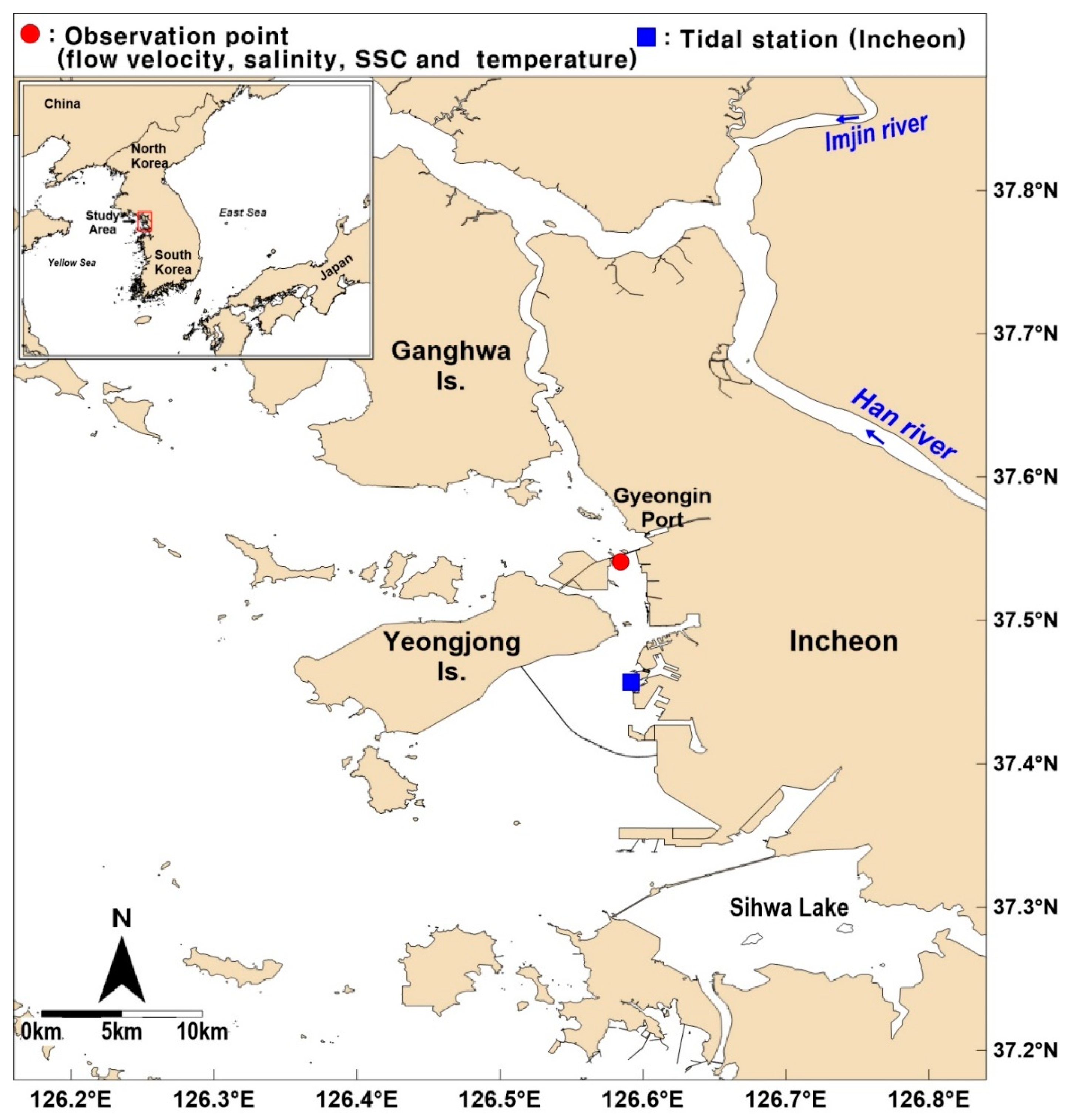
Gyeongin Port area, located on the west coast of Korea, is an area where stratified flow can be observed (Figure 1). Due to macro tidal characteristics (with tidal ranges more than 8.5 m) and complex coastlines (e.g., islands, channels and a large tidal flat), a complex circulation pattern is observed here. The freshwater discharge from the Han River passes through the observation point from the north. Gyeongin Port area is typically well mixed vertically, except during the rainy period in the summer. Because more than 70% of the annual freshwater inflow occurs in the rainy period from June to September, a large amount of freshwater inflow (and sediments) in this period can generate stratification flow [2] and a strong sedimentation tendency. Stratification flow affects the spatial and temporal distribution of water density, salinity and suspended sediment concentration (SSC).
Since the 1990s, field observations have been conducted for salinity distribution. Choi et al. [3] measured the vertical distribution of flow velocity and salinity using an acoustic Doppler current profiler (ADCP) under the conditions of spring/neap tides. Yoon [4] examined tidal cycles of flow velocity and salinities using data observed in the estuary of Gyeonggi Bay and analyzed the relationship between river discharge and salinity distribution. An empirical equation of salt infiltration distance was presented, considering the tidal flow, river discharge and topographical effects. Yoon and Woo [5] related vertical stratification to tidal forcing. They found strong vertical stratification of salinity distribution occurred during the neap period while it decreased during the spring period due to vertical turbulent mixing. These field observations were used with numerical modeling to understand the complex circulation patterns in this area (e.g., [2,5]).
In addition to salinity distribution, SSC is one of the parameters needed to determine the characteristics of sediment transport in this region. Because of a strong sedimentation tendency in this study site, SSC is an important parameter to understand the sediment transport mechanism. Especially, considering that most of severe damages and sedimentation events occurs in the monsoon period in Korea, the stratification effect on SSC due to an abrupt increase of freshwater discharge is critical. Despite the importance of the stratified flow effect on SSC, studies on the relationship between stratified flow and SSC are still rare.
In this study, the effect of stratified flow on SSC was examined. We applied an artificial neural network (ANN), one of the data-driven models, to field observation data to find the hydrodynamic parameters that are important to predict SSC in the estuary. Data-driven modeling is an appropriate approach to inductively understand the complex mechanisms in an estuary. An ANN can identify the relationship between input and output data using a learning process resembling that of the human brain. The ANN has been mostly used when cause and effect is not clearly understood but sufficient data is available [6]. Utilizing these advantages, it has been actively used for difficult and complicated coastal sediment studies (e.g., [7,8,9,10,11,12,13]). The present paper aimed to not only provide a general predictor of sediment concentration, but also explore the sediment transport mechanism from the ANN modeling results. To achieve this goal, we investigated the prediction capability with various combinations of input variables. Using this approach, we examined the contribution of each variable for sediment concentration in the stratified flow condition.
This paper is organized as follows. In Section 2, we analyzed the field data focusing on tidal cycle and river discharge. In Section 3, we optimized the ANN structure and explained the procedure for the analysis. In Section 4, we provide the results with the contribution of the hydrodynamic processes forcing the sediment response in the estuary. Last, in Section 5, we summarize the conclusions.
2. Field Observation
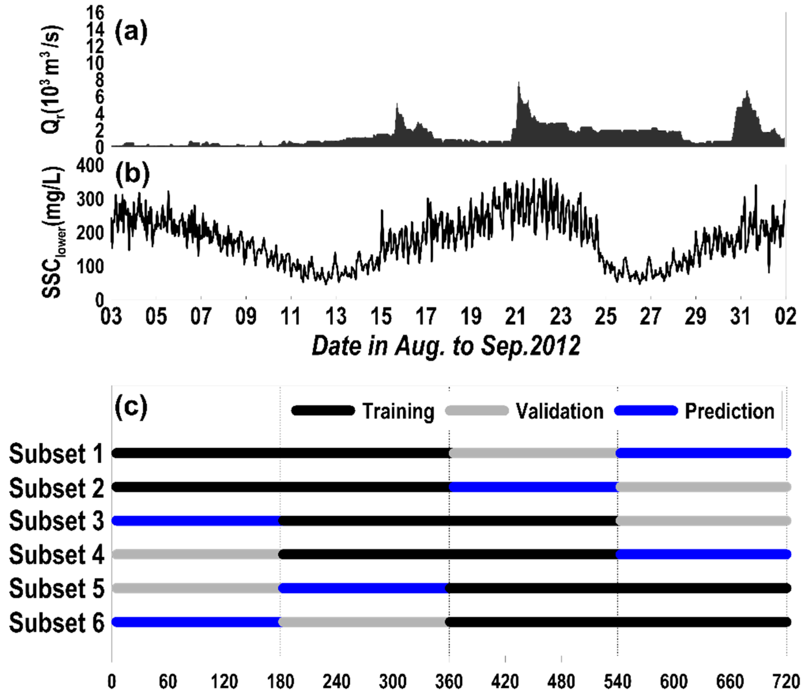
The observation point was located on Gyeongin Port area as shown in Figure 1. The water depth (h) of the measurement was DL (−) 9.6 m. The maximum tidal current was more than 2 m/s and showed ebb-dominance characteristics [5]. The Incheon Regional Maritime Affairs and Fisheries Office conducted observations of the hydrodynamic and sedimentation characteristics (e.g., flow velocity, suspended sediment concentration, water temperature, salinity and wave heights) from 2012 to 2015. In this study, the observation results of the summer of 2012 (3 August 2012 to 2 September 2012), which have few missing data and outliers, were used. In this period, there was a flood event (due to Typhoon Bolaven) in 2012 and, therefore, the effect of abrupt river discharge on the hydrodynamic process in the estuary can be analyzed.
For the observation of flow velocity and suspended sediment concentration, 300 data (sampling rates of 0.5 Hz) were obtained for 10 min using an acoustic Doppler current profiler (ADCP, 600 kHz). ADCP measures the intensity of backscatter as echo intensity from sediment particles. Simple linear regression analysis was used to estimate the SSC using the sampled sediment concentration as a reference. Each set of 300 data was averaged for obtaining the average flow velocity and direction. The upper and lower observation points for the ADCP were set to 0.2 h and 0.8 h from the water surface to the bottom, respectively. A CTD(Conductivity-Temperature-Depth Profiler)-Diver was used for observation of water temperature and salinity. The upper observation point for the CTD-Diver was set to 1 m below the water surface, and the lower observation point was set to 0.5 m above the seabed. Observations of water temperature and salinity were realized at 10 min intervals over a 30-day period. The tide elevation was determined based on data from the Incheon tidal station of the Korea Hydrographic and Oceanographic Agency (KHOA), and it was observed at 1 min intervals during the same period as that of the other observed characteristics. More details of the field observation are referred to in the report published by the Incheon Regional Maritime Affairs and Fisheries Office. [14]
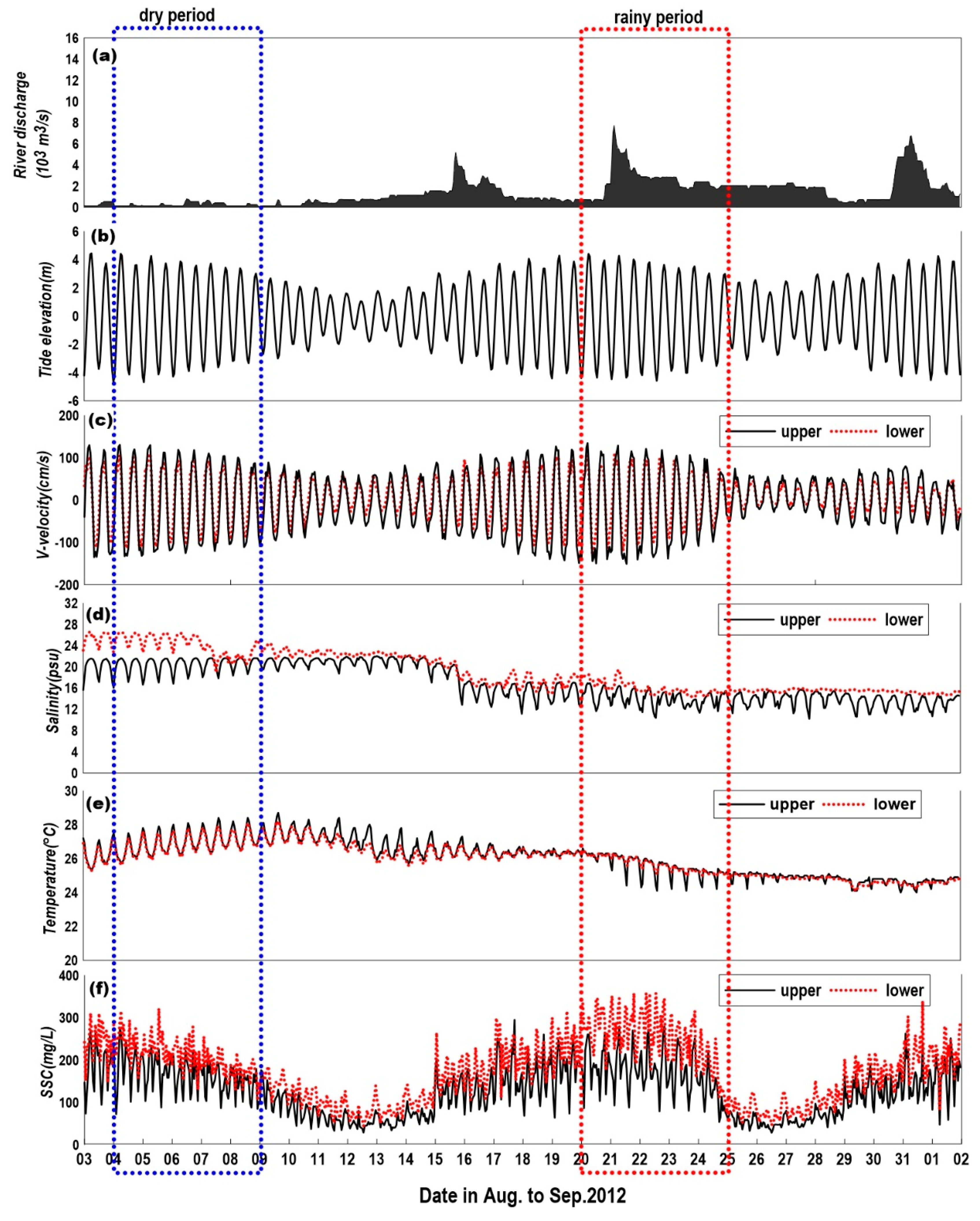
Figure 2 presents a plot of the observations during the summer of 2012 (3 August 2012 to 2 September 2012). Figure 2a shows a freshwater discharge from the Han River. The real-time hydrological data (1 h data) was provided by the Ministry of Environment’s Han River Flood Control Center (http://www.hrfco.go.kr). The overall average flow discharge was 1395.5 m3/s, but the flow rates in the dry period (4–9 August 2012) and in the rainy period (20–25 August 2012) were 248.9 m3/s and 2577.7 m3/s, respectively, showing a difference of 1 order of magnitude. Figure 2b shows the water level. The maximum tide difference was observed to be 8.8 m, showing a significant difference between the spring tide (e.g., 20 August) and neap tide (e.g., 13 August). Figure 2c–f shows the flow velocity, suspended sediment concentration, salinity and water temperature. Note that there are some different features of the upper and lower observations during the dry and rainy periods.
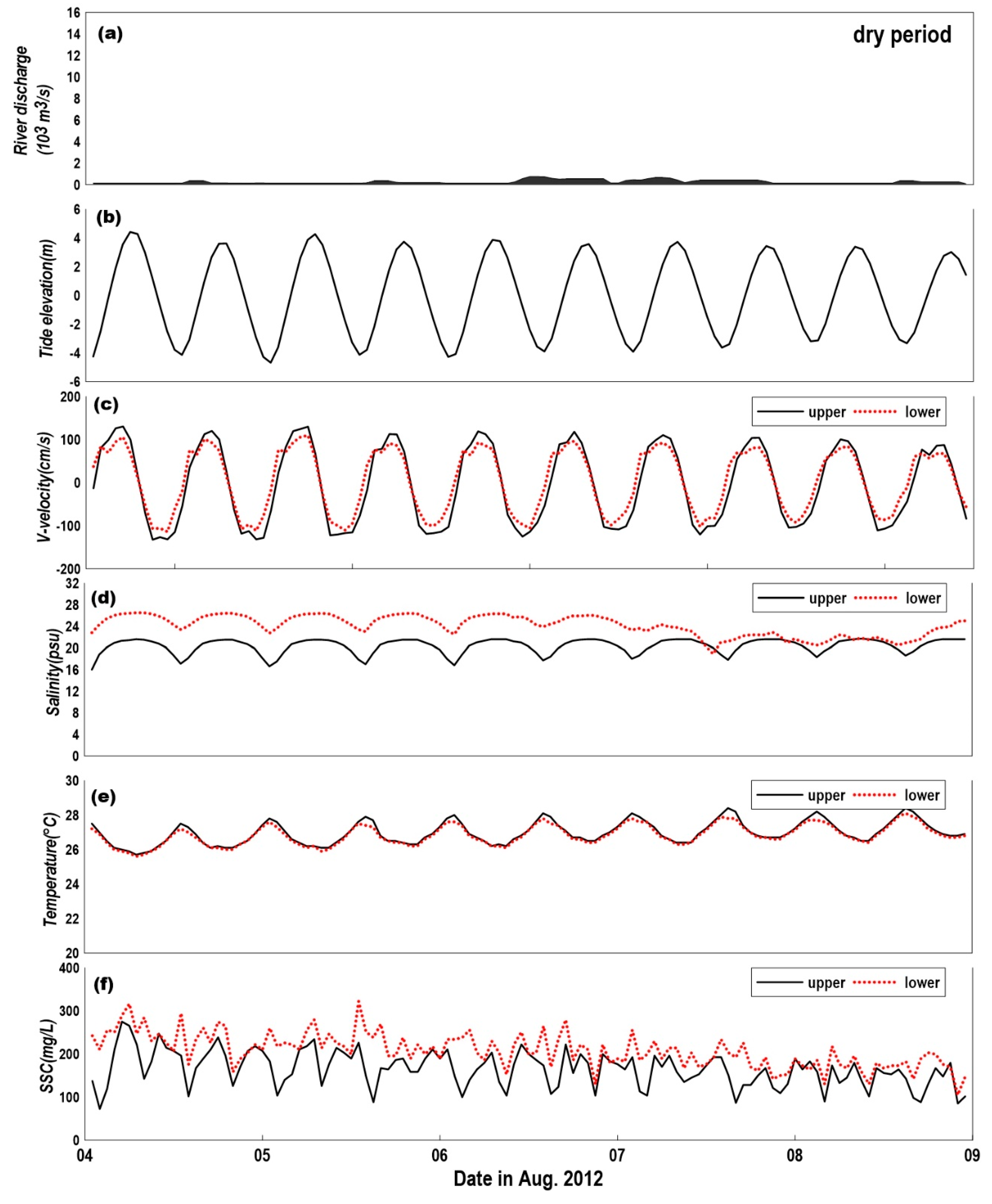
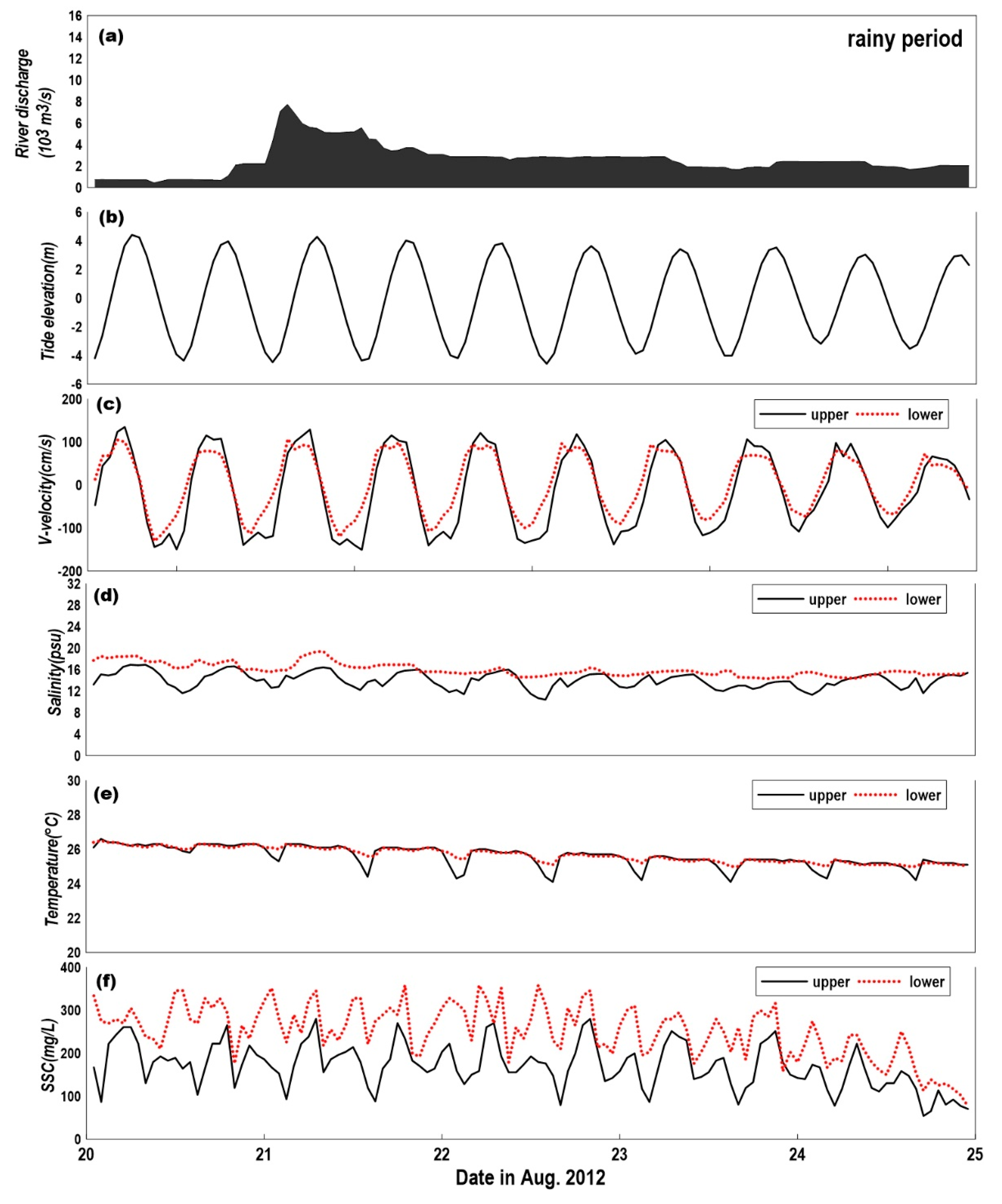
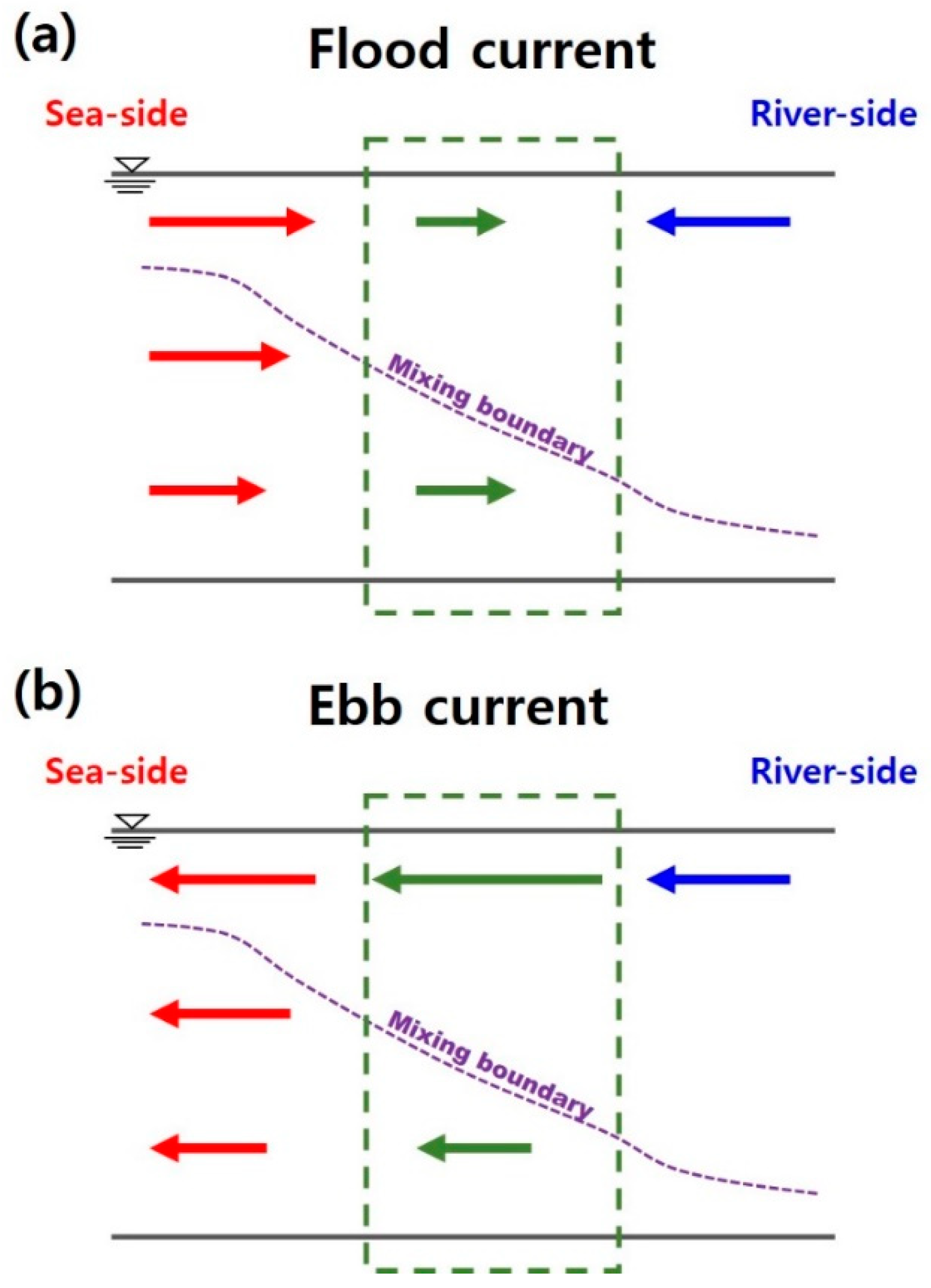
Figure 3 and Figure 4 show close-ups for the dry and rainy periods in Figure 2. Both the dry and rainy periods were set to have 10 tidal cycles with the same phase from the spring tide to neap tide. The difference in the flow velocity between the flood tide and ebb tide was smaller than 10 cm/s during the dry period, while the difference in flow velocity between the flood tide and ebb tide was higher than 20 cm/s in the rainy period. Here, (+) of the flow velocity means flood tide to North and (−) means ebb tide to South. A large flow velocity during ebb tide was shown in the upper layer for the rainy period, as seen in Figure 3c. It can be inferred that this is the result of an increase in the flow velocity in the surface (upper) layer when the tidal current is in the same direction as the river discharge direction during ebb tide. This increase in flow velocity in the ebb tide is illustrated in Figure 5.
Table 1 lists the averaged flow velocity for the upper/lower points, dry/rainy period and flood/ebb tides. The average flow velocity in ebb tide was faster than that in flood tide. The vertical flow velocity ratios, defined as the upper flow velocities divided by the lower flow velocities, were 1.16 for flood tide and 1.26 for the ebb tide in the dry period. However, in the rainy period, the vertical flow velocity ratios were 1.19 for the flood tide and 1.48 for the ebb tide. As the freshwater discharge from the Han river increases, the flow velocity in the upper layer appears to be large in the ebb tide, whereas the flow velocity in the lower layer is constant, even in the ebb tide. This implies that the abruptly increased amount of freshwater from the Han river in the rainy period flows over the heavier seawater with vertically stratified characteristics.
Figure 3d and Figure 4d show the salinity of the upper/lower points for the dry and rainy periods, respectively. The average salinity was 20.4 to 24.2 psu in the dry period and 14.0 to 15.7 psu in the rainy period. The smaller salinity in the rainy period shows the influence of the freshwater flow from the river. During the dry period, periodic changes in salinity appeared in accordance with the tidal phase, whereas the periodicity was weak during the rainy period. The salinity in the lower point shows little dependency on tidal cycle, indicating that the vertical mixing is very limited owing to stratification. This tendency can also be found in Figure 4e, where the water temperature in the lower point was not in phase with that in the upper point during the rainy period, whereas the water temperatures in the upper and lower points were in phase in the dry period, as shown in Figure 3e. Overall, it was found that the stratification feature is formed in the rainy period because of the abruptly increased amount of freshwater from the river.
Figure 3f and Figure 4f show the SSC of the upper/lower points for the dry and rainy periods, respectively. In the dry period, the SSC in the lower point (204.1–208.7 mg/L) was 30% larger than that in the upper point (155.6–173.3 mg/L). In the rainy period, the SSC in the lower point (246.7–247.2 mg/L) was 50% larger than that in the upper point (164.8–169.1 mg/L). There was a 20% increase of SSC in the lower layer during the rainy period, although the SSCs in the upper point for both the dry and rainy periods were similar. It can be inferred that the vertical mixing was reduced due to the activated stratified flow during the rainy period, and therefore, the suspended sediments in the lower layer could not be transported upwards.
3. Modeling of Artificial Neural Network
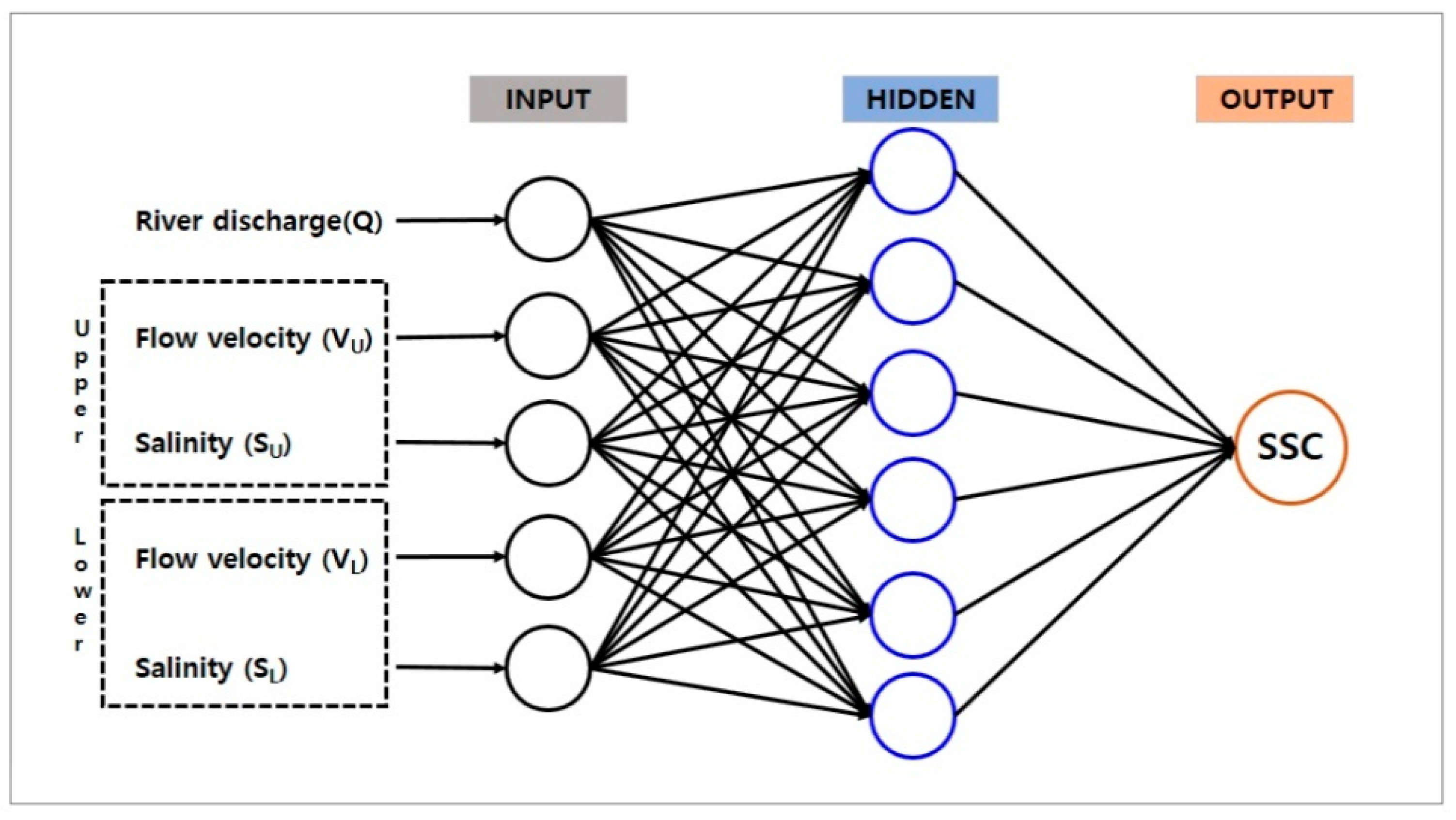
Figure 6 shows the architecture of the ANN model in the present study. Based on the framework of the ANN model developed by Yoon et al. [9], we set a new configuration for the observed field data sets. The ANN architecture is a two-layer feed forward with one hidden layer and one output layer, and the model is calculated with a back-propagation algorithm (Levenberg-Marquardt). The input layer consists of the various combinations of hydrodynamic input data including river discharge, flow velocity and salinity. To account for the time history of input data, four previous time steps of each input parameter are also used. The output layer consists of the SSC at the lower point. These input and output data sets consist of 30 days of data at 1 h intervals, with a total of 720 data points.
Input data and the neurons in the hidden layer are interconnected with weights and bias. Then, the information in the hidden layer is transferred to the output layer with another transfer function. The net input, n1, which is used for the hidden layer can be expressed as (Hagan et al. [15]):
where W is the weight matrix, p is the input and b is the bias. Note that the bold letters represent vectors. The superscript 1 indicates the hidden layer and superscript 2 indicates the output layer. In the weight matrix (W), the first index indicates the neuron destination for that weight and the second index indicates the source of the signal fed to the neuron. The net input, n1, is fed into the hidden layer with the tansig transfer function:
where a1 is the neuron output of the hidden layer. Then, the neuron output from the hidden layer (a1) is used for the output layer with the linear transfer function:
where a2 is the neuron output from the output layer. More details about the ANN model are referred to Yoon et al. [10].
Table 2 lists the cases of input combinations, categorizing them into four groups. Group 1 consists of flow velocity in the lower point. Group 2 consists of river discharge and salinity in addition to flow velocity. Group 3 consists of salinity in addition to flow velocity and river discharge. Group 4 includes hydrodynamic parameters in the upper point, such as flow velocity and salinity, in addition to the hydrodynamic parameters in the lower point. River discharge is abbreviated as Q, flow velocity is abbreviated as V and salinity is abbreviated as S. The lower subscripts L and U represent the lower and upper measurement points. For instance, QVLSLVU represents the conditions including river discharge, flow velocity at the lower point, salinity at the lower point and flow velocity at the upper point.
Figure 7 shows the subset for training, validation and prediction for ANN modeling. Out of the 720 data observed at 1 h intervals for 30 days, 360 data (50% of the total data) were used for training, 180 data (25% of the total data) were used for verification, and 180 data (25% of the total data) were used for prediction. The tests were repeated by changing the training, validation and prediction sets in the whole data set following the so-called bootstrapping technique (e.g., [6,9,10]).
Because the back-propagation ANN is sensitive to the initial weights and biases, it is important to find the proper initial weights and biases for the prediction. Following the procedure by Oehler et al. [9], the ANN was initialized 22 times with random weights and biases. Out of the 22 observations, the weight and bias of the best case in the training and validation set, that with a minimum mean square error (MSE), were kept, and were applied for the prediction set. This approach accounts for the 10% best cases with a confidence of 90%, assuming that the random initial weights and biases follow a normal distribution [9,10].
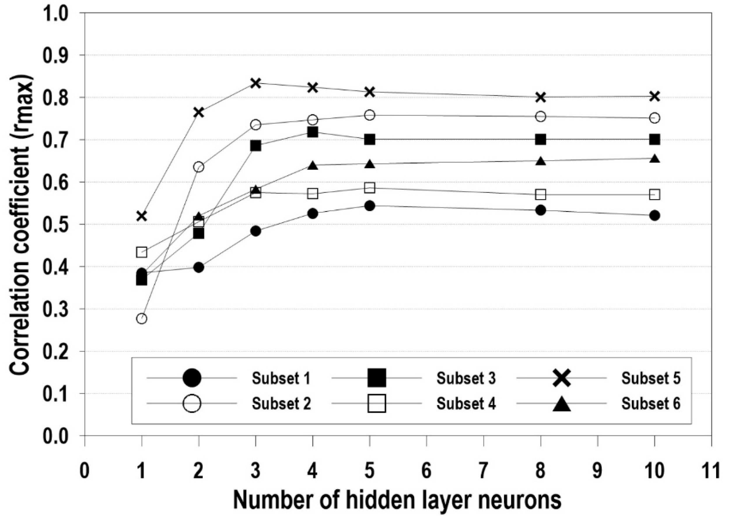
Figure 8 shows the performance of the ANN with various numbers of neurons. The ANN results are dependent on the number of neurons in the hidden layers. To optimize the number of neurons in the hidden layer, we tested the sensitivity for different number of neurons (1, 2, 3, 4, 5, 8, 10) in the hidden layer. We found that three or four neurons showed the best performance for each case. For simplicity, we adopted three neurons in the hidden layer in the present study.
The performance of the ANN was estimated with the maximum correlation coefficient between the measured and predicted SSC. Subset 5 had the highest correlation coefficient with 0.834, whereas Subset 1 had the lowest correlation with r = 0.484. In Subset 5, the SSC was well predicted because the training set included both the flow velocity in the ebb/flood tides and the increase/decrease pattern of the river flow. Other subsets did not include the event of significant river discharge, which leads to insufficient training data to predict the SSC. This indicates the importance of using an appropriate training data set for predicting performance. In this regard, Subset 5 was used for ANN modeling in this study.
Figure 9 shows the time series of the observed and predicted SSC. The time series of SSC is judged to be relatively reproducible. However, as van Maanen et al. [8] and Yoon et al. [10] remarked, the ANN is sometimes difficult to train and predict for extreme values, and there were some discrepancies for extreme values (e.g., September 15 and 17). Nevertheless, the ANN model configured in the study shows a good predictive performance (r = 0.82). More details of the ANN information for this case are given in Appendix A.
4. Results and Discussion
The model performance was evaluated more closely by determining the goodness-of-fit between the measured and predicted SSC with four methods. These methods were the discrepancy ratio (R), root-mean-square-error (RMSE), mean absolute percent error (MAPE), and correlation coefficient (r).
R is defined as:
where xi is the observed value and yi is the predicted value. If the discrepancy ratio is 0, the predicted value is identical to the observed value. If the discrepancy ratio is larger than 0, the predicted value overestimates, and if the discrepancy ratio is smaller than 0, it underestimates. The RMSE also referred to as root-mean-squared deviation (RMSD) is defined as follows:
The RMSE serves to aggregate the magnitudes of the errors in predictions for time series into a single measure of predictive power. The RMSE is always non-negative, and a value of 0 would indicate a perfect fit to the data. In general, a lower RMSE indicates better predictability than a higher one. The MAPE is a measure of prediction accuracy of a prediction method in statistics. For example, in trend estimation, it is used as a loss function for regression problems in machine learning. It usually expresses the accuracy as a ratio defined as follows:
A correlation coefficient (r) is a numerical measure of some type of correlation, meaning a statistical relationship between two values. Several types of correlation coefficient exist, each with their own definition and own range of usability and characteristics. The correlation coefficient is defined as:
where and are the mean of the observed and predicted values, and σx, σy are the standard deviations of x and y, respectively. Several types of correlation coefficient exist, each with their own definition and own range of usability and characteristics. A correlation of −1.0 shows a perfect negative correlation, while a correlation of 1.0 shows a perfect positive correlation. A correlation of 0.0 shows no linear relationship between the movement of the two variables.
Table 3 presents the results of goodness-of-fit between the observed and predicted SSC. The calculated R, RMSE, MAPE and r were ranked in order of highest fit and indexed by score. These indexes were summed and the rank of goodness-of-it was calculated. In general, the hydrodynamic information at the lower point is closely related to the SSC at the lower point (e.g., QVL, QVLSL). Interestingly, when salinity at the upper point was added to the hydrodynamics at the lower point, such as QVLSLSU, this case had the best fit between the observed and predicted SSC. By including the salinity at the upper point, the stratified features of flow were incorporated in the prediction of SSC. This shows, inductively, that the stratification effect caused by the density (or salinity) difference between seawater and freshwater is important to predict SSC in an estuary.
This finding can be helpful for enhancing the performance of numerical modeling in an estuary. For example, this study site is typically assumed vertically well mixed and thus a horizontal, two-dimensional model was used (e.g., Park et al. [2]). However, as noted by Park et al. [2], three-dimensional modeling may differ from the two-dimensional depth-averaged estimates. The stratification effect on SSC is important information to estimate mass transport and sediment transport in the rainy period. As most of severe damage and sedimentation events occur in the monsoon period in Korea, the stratification effect on SSC can be considered in a numerical simulation.
We anticipate that some improvements and additional studies will be needed to develop the present ANN model. A limitation of the present study is that it uses data collected at one study site. Because of the complex structure of the ANN model, it is difficult to apply the configuration (weights and bias) of the present ANN model to other locations. Adding data sets of measured hydrodynamic parameters and sediment responses at other sites can improve the predictability of the ANN model (or any other data-driven predictive model). Moreover, the data set used here contains only one month of time series. Further improvements to the model could include longer data sets with a larger number of events. Finally, future studies will need to analyze additional input parameters such as wind, waves and meteorological factors. In this study, only river discharge, flow velocity and salinity were used as predictors of SSC. However, previous studies have demonstrated that SSC can be affected by wind and water levels, along with salinity and flow velocity [16,17]. Although it is not possible to explain the increase in SSC due to sediment resuspension by wind force alone, the SSC is increased by wind-induced waves even at high tide [18]. Meteorological factors such as wind speed, wind direction and precipitation have been found to be the significant driving forces for SSC variation at both the short (minutes) and long (days) time scales [19].
5. Conclusions
In this study, the characteristics of stratified flow caused by river flow during flooding were analyzed using measured data of tidal currents, river freshwater discharge, salinity and SSC observed in Gyeongin Port, a representative estuary of Korea. Then, using an ANN, one of the data-driven modeling techniques, the effect of stratified flow on the SSC was inductively examined. The conclusions obtained through this research can be summarized as follows.
- It was found that there were stratified flow features of flow velocity, salinity and temperature between the upper and lower layers in the Gyeonin Port area of South Korea. The abruptly increased amount of freshwater from a river in the rainy period flows over the heavier seawater, with vertically stratified characteristics. In addition, even though the periodic changes in salinity and temperature of the surface layer due to the tidal cycle were significant, changes in the lower layer were small, and the flow characteristics of the stratified flow could be confirmed.
- The SSC in the estuary shows a relatively high correlation with the discharge from the river, the flow velocity at the surface and bottom and the salt concentration at the surface and bottom. When the freshwater flow direction and the tidal flow direction are the same, there is a relatively high correlation between the SSC and the hydrodynamic parameters in both the surface and bottom layers. During flood tide, when the directions of the freshwater and tidal flows are opposite, the SSC in the lower layer has a lower correlation with hydrodynamic parameters due to the stratification effect.
- An ANN, one of the data-driven modeling techniques, was used to analyze the correlation between SSC and hydrodynamic factors. When the number of neurons was 3–4, it had the best performance, and it was found that the model’s ability to predict SSC was improved when the training section included the abrupt river discharge due to flooding. This implies that the stratification effect due to the rapid discharge from a river is important in the prediction of SSC in an estuary.
- The model performance was evaluated more closely by determining the goodness-of-fit between the measured and predicted SSC with four methods. The four goodness-of-fit methods were R, RMSE, MAPE and correlation coefficient (r). The results of goodness-of-fit were ranked and indexed by the score. The case including the discharge from the river, flow velocity near the bottom and surface and bottom salinity showed the best fit between the measured and predicted SSC. In particular, it was found that the highest degree of fitness was obtained from the results considering salinity data of both the surface and bottom layers, which represent the stratification effect. This shows, inductively, that the stratification effect caused by the density difference between seawater and freshwater is important to predict SSC in an estuary.
Author Contributions
Conceptualization, H.-J.S., M.C. and H.-D.Y.; methodology, H.-J.S., M.C. and H.-D.Y.; Investigation, H.-J.S.; writing—original draft preparation, H.-J.S. and H.-D.Y.; writing—review and editing, H.-J.S. and H.-D.Y.; supervision, H.-D.Y.; funding acquisition, H.-D.Y. All authors have read and agreed to the published version of the manuscript.
Funding
This research was supported by the Basic Science Research Program through the National Research Foundation of Korea (NRF) funded by the Ministry of Science, ICT & Future Planning (NRF-2016R1D1A1B03935635).
Conflicts of Interest
The authors declare no conflict of interest.
Appendix A
The weights and bias of hidden layer and output layer for Figure 9 are listed in Table A1 and Table A2, respectively. Five time steps (i-4, i-3, i-2, i-1, i), where i represents the prediction time, of each input parameter are used.

Table A1.
Weight(W1) and bias(b1) matrix of hidden layer (Case: QVLSLSU and Subset 5). The superscript 1 indicates the hidden layer.
Table A1.
Weight(W1) and bias(b1) matrix of hidden layer (Case: QVLSLSU and Subset 5). The superscript 1 indicates the hidden layer.
| Input | W1 | b1 | ||||||||||||||||||||
|---|---|---|---|---|---|---|---|---|---|---|---|---|---|---|---|---|---|---|---|---|---|---|
| Lower Velocity (VL) | River Discharge (Q) | Lower Salinity (SL) | Upper Velocity (VU) | |||||||||||||||||||
| Neuron | i-4 | i-3 | i-2 | i-1 | i | i-4 | i-3 | i-2 | i-1 | i | i-4 | i-3 | i-2 | i-1 | i | i-4 | i-3 | i-2 | i-1 | i | ||
| 1st | −0.545 | −0.562 | −0.441 | 0.275 | 0.099 | 0.057 | 0.117 | −0.158 | −0.295 | 0.049 | 0.324 | 0.451 | 0.345 | −0.507 | −0.035 | −0.351 | 0.365 | −0.390 | 0.266 | 0.007 | 1.479 | |
| 2nd | 0.194 | 0.220 | −0.254 | 0.081 | −0.557 | −0.459 | −0.558 | −0.377 | −0.217 | 0.327 | 0.172 | −0.084 | 0.044 | −0.224 | −0.312 | −0.538 | −0.542 | 0.123 | −0.165 | 0.299 | 0.000 | |
| 3rd | −0.489 | −0.585 | −0.217 | 0.018 | −0.174 | −0.268 | −0.552 | −0.228 | 0.099 | −0.150 | 0.061 | 0.087 | 0.569 | −0.141 | −0.211 | −0.570 | 0.474 | 0.027 | 0.304 | −0.162 | −1.479 | |
Table A2.
Weight(W2) and bias(b2) matrix of output layer (Case: QVLSLSU and Subset 5). The superscript 2 indicates the output layer.
Table A2.
Weight(W2) and bias(b2) matrix of output layer (Case: QVLSLSU and Subset 5). The superscript 2 indicates the output layer.
| Output | W2 | b2 | |||
|---|---|---|---|---|---|
| Neuron | 1st Neuron Output | 2nd Neuron Output | 3rd Neuron Output | ||
| 1st | 0.850 | 0.802 | 0.103 | 0.042 | |
References
- Nielsen, P. Coastal and Estuarine Processes; World Scientific: Singapore, 2009; pp. 1–341. [Google Scholar]
- Park, K.; Oh, J.-H.; Kim, H.-S.; Im, H.-H. Case Study: Mass Transport Mechanism in Kyunggi Bay around Han River Mouth, Korea. J. Hydraul. Eng. 2002, 128, 257–267. [Google Scholar] [CrossRef]
- Choi, N.W.; Woo, S.B. Study on lateral flow distribution and momentum analysis at flood season and neap tide of the Seokmo Channel in the Han River estuary. Korean Soc. Coast. Ocean Eng. 2012, 24, 390–399. [Google Scholar] [CrossRef] [Green Version]
- Yoon, B.I. Estuarine Circulation and Dynamics of a Shallow, Tidally Dominated, Han River Estuary in the Gyeonggi Bay (Doctoral Dissertation); Inha University: Incheon, Korea, 2015. [Google Scholar]
- Yoon, B.I.; Woo, S.-B. The Along-Channel Salinity Distribution and its Response to River Discharge in Tidally-Dominated Han River Estuary, South Korea. In Proceedings of the 8th International Conference on Asian and Pacific Coasts (APAC 2015), Chennai, India, 7–10 September 2015; Volume 116, pp. 763–770. [Google Scholar]
- Van Gent, M.R.A.; Van Den Boogaard, H.F.P.; Pozueta, B.; Medina, J.R. Neural network modeling of wave overtopping at coastal structures. Coast. Eng. 2007, 54, 586–593. [Google Scholar] [CrossRef] [Green Version]
- Singh, A.K.; Deo, M.C.; Sanil Kumar, V. Prediction of littoral drift with artificial neural networks, Hydrology and Earth Systems Sciences. Eur. Geophys. Union 2008, 12, 267–275. [Google Scholar]
- Van Maanen, B.; Coco, G.; Bryan, K.R.; Ruessink, B.G. The use of artificial neural networks to analyze and predict alongshore sediment transport. Nonlinear Process. Geophys. 2010, 17, 395–404. [Google Scholar] [CrossRef]
- Oehler, F.; Coco, G.; Green, M.O.; Bryan, K.R. A data-driven approach to predict suspended-sediment reference concentration under non-breaking waves. Cont. Shelf Res. 2012, 46, 96–106. [Google Scholar] [CrossRef]
- Yoon, H.-D.; Cox, D.T.; Kim, M.K. Prediction of time-dependent sediment suspension in the surf zone using artificial neural network. Coast. Eng. 2013, 71, 78–86. [Google Scholar] [CrossRef]
- Kerh, T.; Lu, H.; Saunders, R. Investigating Nonlinear Shoreline Multiperiod Change from Orthophoto Map Information by Using a Neural Network Model. Math. Probl. Eng. 2014, 3, 1–9. [Google Scholar] [CrossRef]
- Demirci, M.; Üneş, F.; Aköz, M.S. Prediction of cross-shore sandbar volumes using neural network approach. J. Mar. Sci. Technol. 2015, 20, 171–179. [Google Scholar] [CrossRef]
- Sahin, C.; Gruner, H.A.A.; Ozturk, M.; Sheremet, A. Floc size variability under strong turbulence: Observations and artificial neural network modeling. Appl. Ocean. Res. 2017, 68, 130–141. [Google Scholar] [CrossRef] [Green Version]
- Incheon Regional Office of Ocean and Fisheries. Field Monitoring Report of Incheon Gyeongin Port (in Korean); Incheon Regional Office of Ocean and Fisheries: Incheon, Korea, 2016; pp. 1–1190. [Google Scholar]
- Hagan, M.T.; Demuth, H.B.; Beale, M. Neural Network Design; PWS Publishing: Boston, MA, USA, 1996; pp. 1–736. [Google Scholar]
- Schoellhamer, D.H. Sediment resuspension mechanisms in old Tampa bay, Florida. Estuary. Cont. Shelf Res. 1995, 40, 603–620. [Google Scholar]
- Lawrence, D.; Dagg, M.J.; Liu, H.B.; Cummings, S.R.; Ortner, P.B.; Kelble, C. Wind events and benthic-pelagic coupling in a shallow Subtropical bay in Florida. Mar. Ecol. Prog. Ser. 2004, 266, 1–13. [Google Scholar] [CrossRef] [Green Version]
- Chen, Z.; Hu, C.; Muller-Karger, F.E.; Luther, M.E. Short-term variability of suspended sediment and phytoplankton in Tampa bay, Florida: Observations from a coastal oceanographic tower and ocean color satellites. Estuar. Coast. Shelf Sci. 2010, 89, 62–72. [Google Scholar] [CrossRef]
- Talke, S.A.; Stacey, M.T. Suspended sediment fluxes at an intertidal flat: The shifting influence of wave, wind, tidal, and freshwater forcing. Cont. Shelf Res. 2008, 28, 710–725. [Google Scholar] [CrossRef] [Green Version]
Figure 1.
Location of observation point.

Figure 2.
Classification of the dry and the rainy period during the summer in 2012: (a) freshwater discharge from Han River, (b) tide elevation of Incheon station, (c) horizontal flow velocity (+: north, −: south), (d) salinity, (e) temperature, and (f) SSC.
Figure 2.
Classification of the dry and the rainy period during the summer in 2012: (a) freshwater discharge from Han River, (b) tide elevation of Incheon station, (c) horizontal flow velocity (+: north, −: south), (d) salinity, (e) temperature, and (f) SSC.

Figure 3.
Time series of the observed data during the dry period: (a) freshwater discharge from Han River, (b) tide elevation of Incheon station, (c) horizontal flow velocity (+: north, −: south), (d) salinity, (e) temperature, and (f) SSC.
Figure 3.
Time series of the observed data during the dry period: (a) freshwater discharge from Han River, (b) tide elevation of Incheon station, (c) horizontal flow velocity (+: north, −: south), (d) salinity, (e) temperature, and (f) SSC.

Figure 4.
Time series of the observed data during the rainy period: (a) freshwater discharge from Han River, (b) tide elevation of Incheon station, (c) horizontal flow velocity (+: north, −: south), (d) salinity, (e) temperature, and (f) SSC.
Figure 4.
Time series of the observed data during the rainy period: (a) freshwater discharge from Han River, (b) tide elevation of Incheon station, (c) horizontal flow velocity (+: north, −: south), (d) salinity, (e) temperature, and (f) SSC.

Figure 5.
Vertical profile of current during (a) flood tide and (b) ebb tide.

Figure 6.
Structure of ANN.

Figure 7.
Subset for training, validation and prediction: (a) freshwater discharge from Han river, (b) SSC at the lower point, (c) subsets.
Figure 7.
Subset for training, validation and prediction: (a) freshwater discharge from Han river, (b) SSC at the lower point, (c) subsets.

Figure 8.
Variation of correlation coefficients according to number of hidden layer neurons.

Figure 9.
Time series of observed SSC (circle) and predicted SSC (solid line) in the prediction set. Input Case QVLSLSU and Subset 5 are used for the training, validation and prediction.
Figure 9.
Time series of observed SSC (circle) and predicted SSC (solid line) in the prediction set. Input Case QVLSLSU and Subset 5 are used for the training, validation and prediction.

Table 1.
Comparison of the ratio of the averaged upper flow velocity to the averaged lower flow velocity.
Table 1.
Comparison of the ratio of the averaged upper flow velocity to the averaged lower flow velocity.
| Tidal Period | Dry Period | Rainy Period | ||||||||||
|---|---|---|---|---|---|---|---|---|---|---|---|---|
| Flood Tide | Ebb Tide | Flood Tide | Ebb Tide | |||||||||
| Low | Up | Up/Low | Low | Up | Up/Low | Low | Up | Up/Low | Low | Up | Up/Low | |
| 1 | 70.5 | 78.2 | 1.11 | 76.9 | 105.3 | 1.37 | 73.0 | 92.8 | 1.27 | 67.8 | 95.9 | 1.41 |
| 2 | 85.2 | 91.1 | 1.07 | 76.4 | 103.0 | 1.35 | 69.7 | 78.6 | 1.13 | 66.4 | 112.2 | 1.69 |
| 3 | 70.0 | 90.0 | 1.29 | 77.0 | 86.0 | 1.12 | 71.8 | 74.6 | 1.04 | 64.5 | 109.2 | 1.69 |
| 4 | 59.9 | 82.7 | 1.38 | 70.0 | 84.3 | 1.20 | 69.0 | 80.6 | 1.17 | 66.1 | 97.2 | 1.47 |
| 5 | 71.2 | 74.2 | 1.04 | 69.8 | 94.2 | 1.35 | 67.8 | 75.0 | 1.11 | 56.7 | 86.3 | 1.52 |
| 6 | 73.5 | 77.2 | 1.05 | 66.0 | 85.7 | 1.30 | 52.5 | 72.2 | 1.38 | 53.9 | 76.0 | 1.41 |
| 7 | 57.3 | 70.3 | 1.23 | 64.1 | 75.2 | 1.17 | 47.6 | 58.3 | 1.22 | 49.8 | 65.1 | 1.31 |
| 8 | 53.1 | 68.3 | 1.29 | 68.0 | 77.0 | 1.13 | 39.7 | 48.1 | 1.21 | 44.2 | 56.2 | 1.27 |
| 9 | 58.5 | 61.6 | 1.05 | 56.8 | 80.6 | 1.42 | - | - | - | - | - | - |
| Avg. | 66.1 | 76.8 | 1.16 | 69.5 | 87.6 | 1.26 | 60.5 | 71.8 | 1.19 | 59.0 | 87.2 | 1.48 |
Table 2.
Case of input data. Closed and open circles denote used and unused input data, respectively.
Table 2.
Case of input data. Closed and open circles denote used and unused input data, respectively.
| Group | Case | River Discharge | Low. Flow Velocity | Low. Salinity | Up. Flow Velocity | Up. Salinity |
|---|---|---|---|---|---|---|
| 1 | VL | ○ | ● | ○ | ○ | ○ |
| 2 | QVL | ● | ● | ○ | ○ | ○ |
| VLSL | ○ | ● | ● | ○ | ○ | |
| 3 | QVLSL | ● | ● | ● | ○ | ○ |
| 4 | QVLSLVU | ● | ● | ● | ● | ○ |
| QVLSLSU | ● | ● | ● | ○ | ● | |
| QVLVUSU | ● | ● | ○ | ● | ● |
Table 3.
Results of goodness-of-fit between observed and predicted SSC.
| Group | Case | R 1 | RMSE 2 | MAPE 3 | r 4 | Sum. of Rank Index | Fitness Rank |
|---|---|---|---|---|---|---|---|
| 1 | VL | 7 (1.26) | 7 (54.2) | 7 (36.3) | 7 (0.738) | 28 | 7 |
| 2 | QVL | 6 (1.19) | 4 (47.1) | 6 (29.3) | 3 (0.796) | 19 | 5 |
| VLSL | 4 (1.15) | 2 (45.4) | 3 (27.3) | 4 (0.793) | 13 | 2 | |
| 3 | QVLSL | 3 (1.14) | 3 (45.9) | 2 (27.0) | 5 (0.788) | 13 | 2 |
| 4 | QVLSLVU | 5 (1.15) | 5 (47.2) | 5 (28.8) | 6 (0.771) | 21 | 6 |
| QVLSLSU | 1 (1.02) | 1 (44.6) | 1 (25.6) | 1 (0.820) | 4 | 1 | |
| QVLVUSU | 2 (0.91) | 6 (48.6) | 4 (27.5) | 2 (0.820) | 14 | 4 |
1 discrepancy ratio; 2 root-mean-square-error; 3 mean absolute percent error; 4 correlation coefficient.
© 2020 by the authors. Licensee MDPI, Basel, Switzerland. This article is an open access article distributed under the terms and conditions of the Creative Commons Attribution (CC BY) license (http://creativecommons.org/licenses/by/4.0/).
Share and Cite
MDPI and ACS Style
Seo, H.-J.; Cho, M.; Yoon, H.-D. Data-Driven Analysis of Stratified Flow Effect on Suspended Sediment Concentration in an Estuary. J. Mar. Sci. Eng. 2020, 8, 606. https://doi.org/10.3390/jmse8080606
AMA Style
Seo H-J, Cho M, Yoon H-D. Data-Driven Analysis of Stratified Flow Effect on Suspended Sediment Concentration in an Estuary. Journal of Marine Science and Engineering. 2020; 8(8):606. https://doi.org/10.3390/jmse8080606
Chicago/Turabian StyleSeo, Heui-Jung, Minsang Cho, and Hyun-Doug Yoon. 2020. "Data-Driven Analysis of Stratified Flow Effect on Suspended Sediment Concentration in an Estuary" Journal of Marine Science and Engineering 8, no. 8: 606. https://doi.org/10.3390/jmse8080606
Note that from the first issue of 2016, this journal uses article numbers instead of page numbers. See further details here.