Investigation of Optimal Coupling Velocities of the Sample and Sheath Flows for Hydrodynamic Focusing

 ,
,  and
and 
Abstract
:1. Introduction
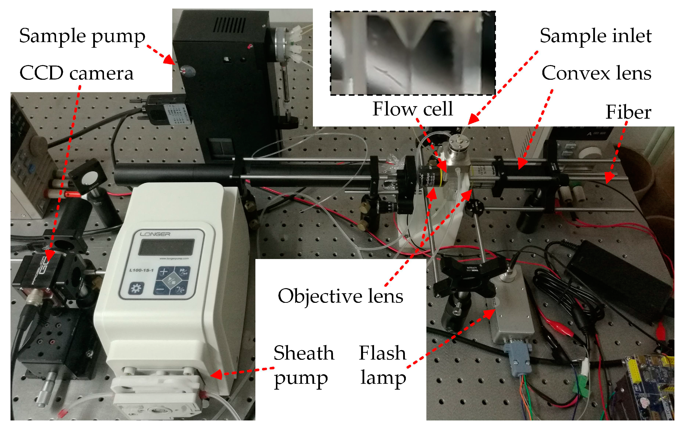
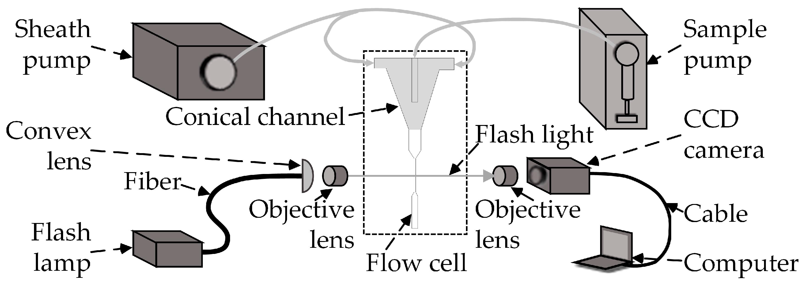
2. System Overview
3. Theoretical Optimisation of the Coupling Velocities
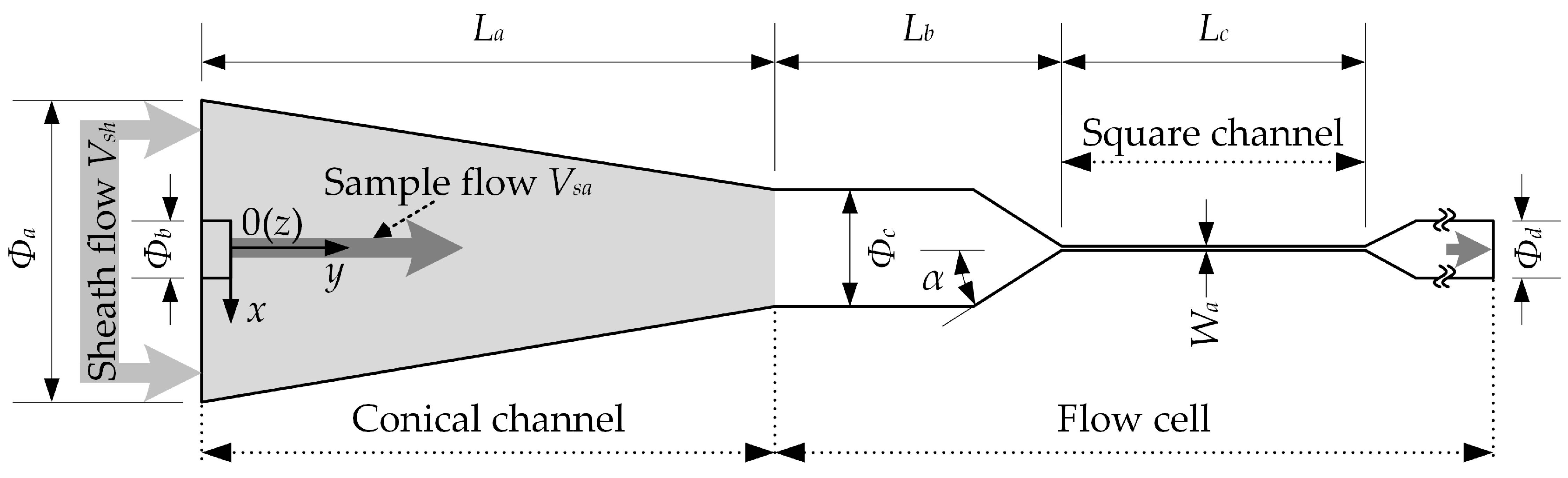
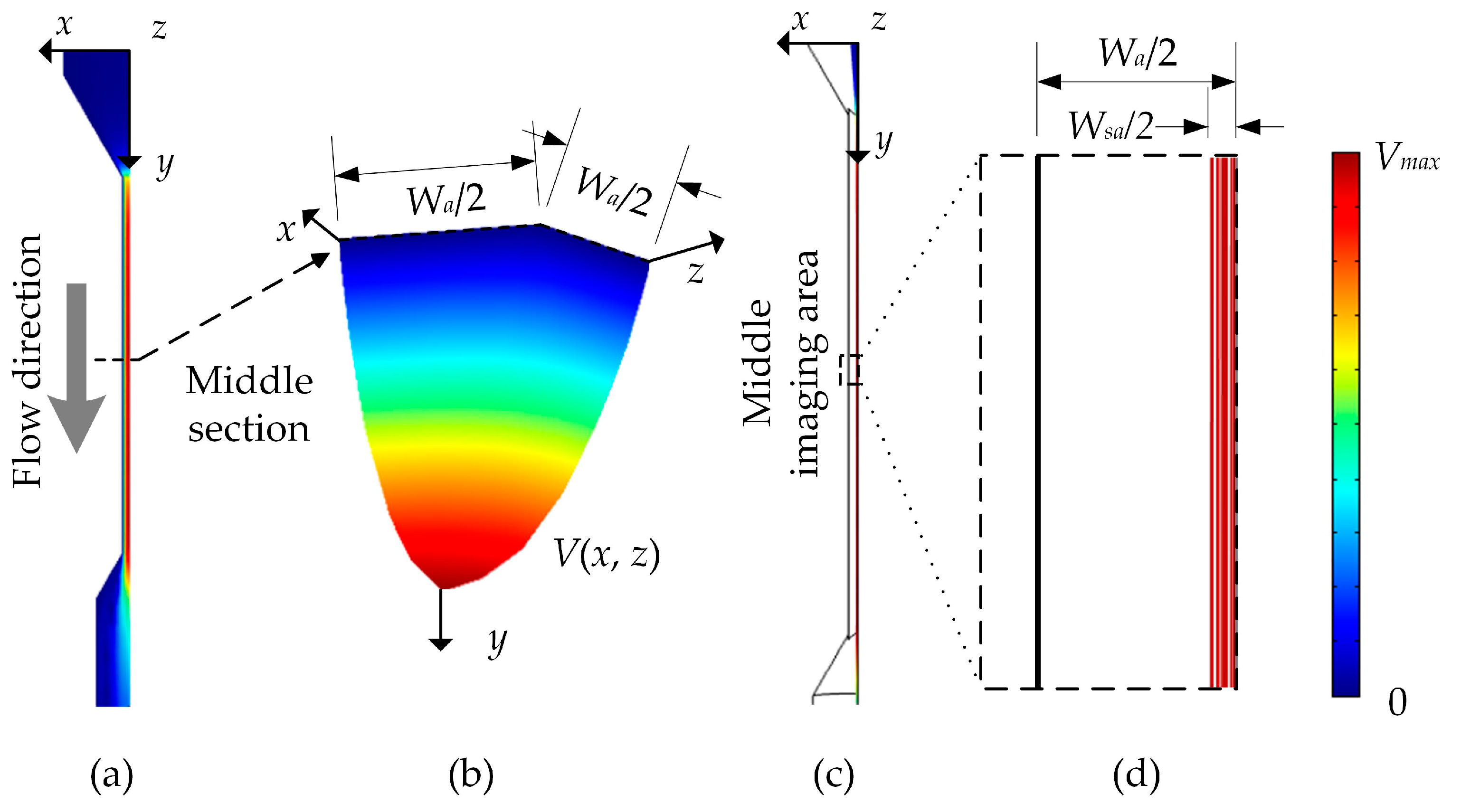
3.1. Theoretical Model
- The fluid is Newtonian. For a Newtonian fluid subjected to shear, the resulting strain rate εxy is linearly related to the applied stress τxy, which is numerically expressed as τxy = 2µεxy [18].
- The flow in the micro-channel is steady.
- The density of the fluid in the channel is uniform.
3.2. Theoretical Simulation
3.2.1. Parameters for Guiding and Evaluating the Theoretical Simulation
3.2.2. Details of the Theoretical Simulation
3.3. Theoretical Simulation Results
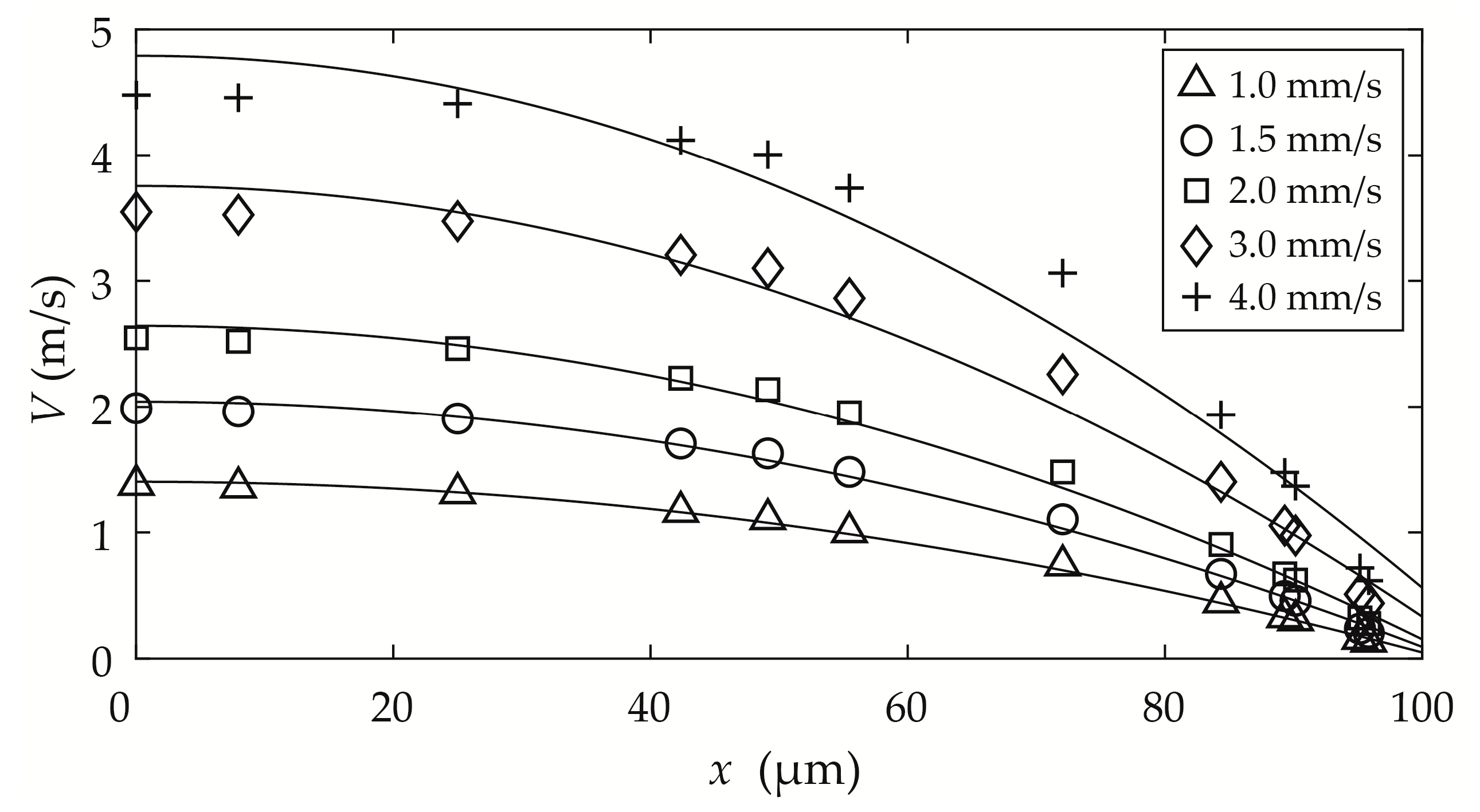
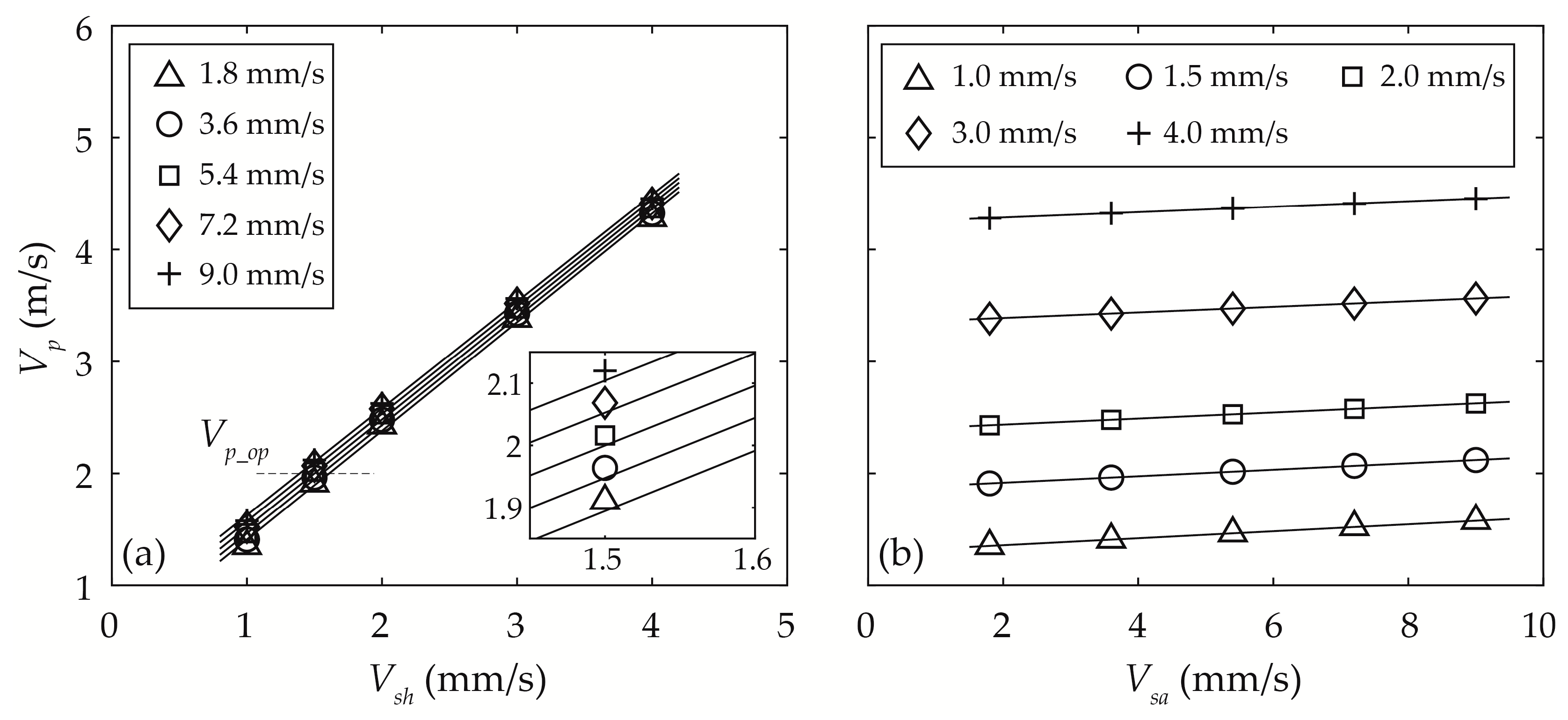
3.3.1. Sample Particle Velocity Vp
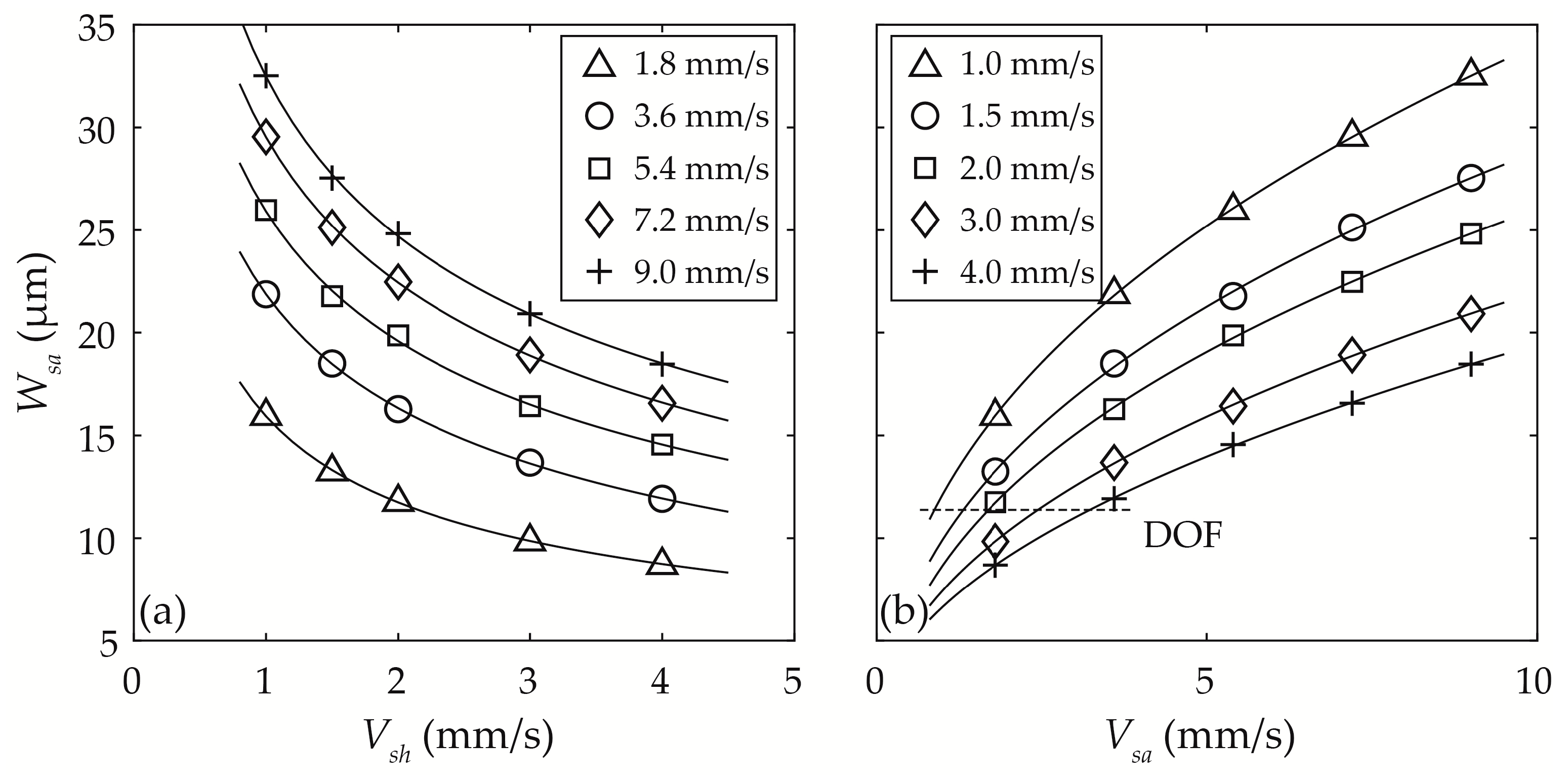
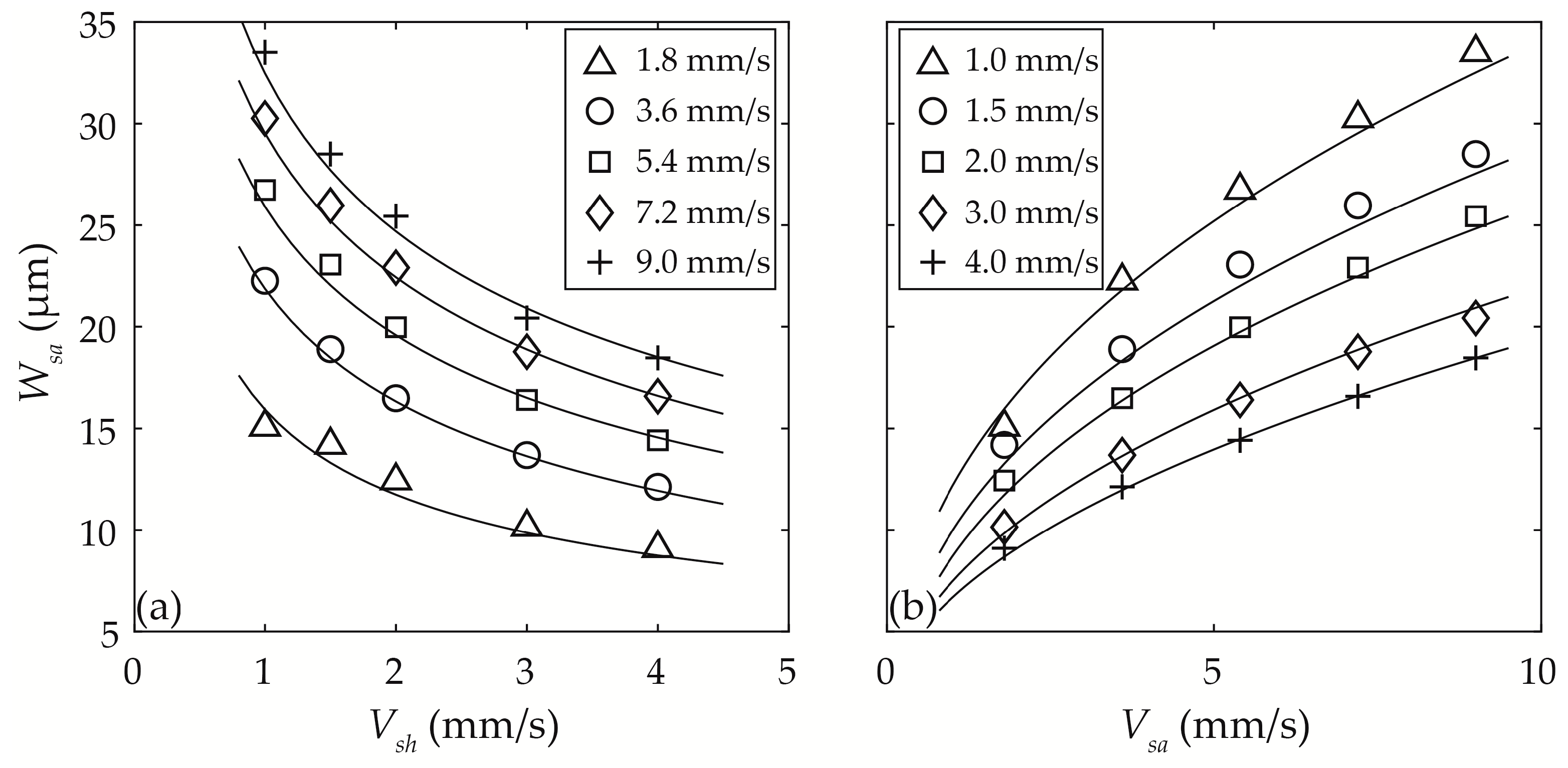
3.3.2. Width of the Sample Particle Stream Wsa
3.3.3. Optimisation of Vsh and Vsa
4. Experimental Verification
4.1. Experiments
4.2. Experimental Results
4.2.1. Smear of Sample Particles
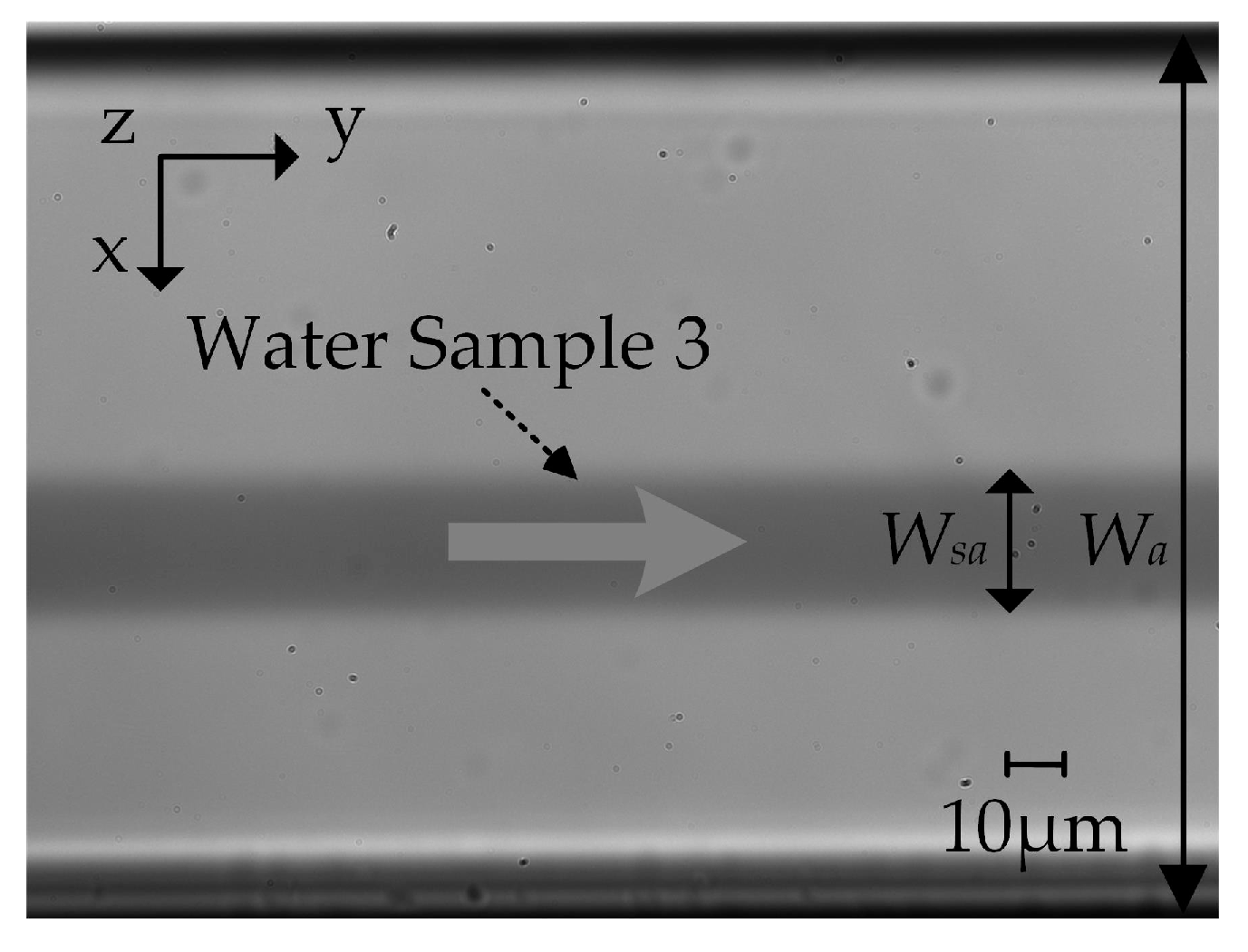
4.2.2. Width of the Focused Sample Flow Stream Wsa
5. Conclusions
Author Contributions
Funding
Acknowledgments
Conflicts of Interest
References
- Altschuler, S.J.; Wu, L.F. Cellular heterogeneity: Do differences make a difference? Cell 2010, 141, 559–563. [Google Scholar] [CrossRef] [PubMed] [Green Version]
- Das, D.; Biswas, K.; Das, S. A microfluidic device for continuous manipulation of biological cells using dielectrophoresis. Med. Eng. Phys. 2014, 36, 726–731. [Google Scholar] [CrossRef] [PubMed]
- Jiang, H.; Weng, X.; Li, D. A novel microfluidic flow focusing method. Biomicrofluidics 2014, 8, 054120. [Google Scholar] [CrossRef] [Green Version]
- Collins, D.J.; Morahan, B.; Garcia-Bustos, J. Two-dimensional single-cell patterning with one cell per well driven by surface acoustic waves. Nat. Commun. 2015, 6, 1–11. [Google Scholar] [CrossRef] [Green Version]
- Ha, B.H.; Lee, K.S.; Jung, J.H. Three-dimensional hydrodynamic flow and particle focusing using four vortices Dean flow. Microfluid. Nanofluidics 2014, 17, 647–655. [Google Scholar] [CrossRef]
- Versaci, M.; Palumbo, A. Magnetorheological fluids: Qualitative comparison between a mixture model in the extended irreversible thermodynamics framework and an Herschel—Bulkley experimental elastoviscoplastic model. Int. J. Non Linear Mech. 2020, 118, 103288. [Google Scholar] [CrossRef]
- Luo, T.; Fan, L.; Zhu, R. Microfluidic single-cell manipulation and analysis: Methods and applications. Micromachines 2019, 10, 104. [Google Scholar] [CrossRef] [Green Version]
- Hamilton, E.S.; Ganjalizadeh, V.; Wright, J.G. 3D Hydrodynamic Focusing in Microscale Optofluidic Channels Formed with a Single Sacrificial Layer. Micromachines 2020, 11, 349. [Google Scholar] [CrossRef] [Green Version]
- Wang, Q.; Yuan, D.; Li, W. Analysis of hydrodynamic mechanism on particles focusing in micro-channel flows. Micromachines 2017, 8, 197. [Google Scholar] [CrossRef] [Green Version]
- Wang, X.; Zandi, M.; Ho, C.C. Single stream inertial focusing in a straight microchannel. Lab A Chip 2015, 15, 1812–1821. [Google Scholar] [CrossRef]
- Panwar, N.; Song, P.; Tjin, S.C. Sheath-assisted hydrodynamic particle focusing in higher Reynolds number flows. J. Micromechanics Microengineering 2018, 28, 105018. [Google Scholar] [CrossRef]
- Chiu, Y.J.; Cho, S.H.; Mei, Z. Universally applicable three-dimensional hydrodynamic microfluidic flow focusing. Lab A Chip 2013, 13, 1803–1809. [Google Scholar] [CrossRef] [PubMed]
- Mao, X.; Lin, S.C.S.; Dong, C. Single-layer planar on-chip flow cytometer using microfluidic drifting based three-dimensional (3D) hydrodynamic focusing. Lab A Chip 2009, 9, 1583–1589. [Google Scholar] [CrossRef] [PubMed]
- Lee, G.B.; Hung, C.I.; Ke, B.J. Hydrodynamic Focusing for a Micromachined Flow Cytometer. J. Fluids Eng. 2001, 123, 672. [Google Scholar] [CrossRef] [Green Version]
- Lee, G.B.; Chang, C.C.; Huang, S.B. The hydrodynamic focusing effect inside rectangular microchannels. J. Micromechanics Microengineering 2006, 16, 1024. [Google Scholar] [CrossRef]
- Oakey, J.; Applegate, R.W.; Arellano, E. Particle focusing in staged inertial microfluidic devices for flow cytometry. Anal. Chem. 2010, 82, 3862–3867. [Google Scholar] [CrossRef] [Green Version]
- Zhao, J.; You, Z. Microfluidic hydrodynamic focusing for high-throughput applications. J. Micromechanics Microengineering 2015, 25, 125006. [Google Scholar] [CrossRef]
- Stiles, T.; Fallon, R.; Vestad, T. Hydrodynamic focusing for vacuum-pumped microfluidics. Microfluid. Nanofluidics 2005, 1, 280–283. [Google Scholar] [CrossRef]
- Cornish, R.J. Flow in a pipe of rectangular cross-section. Proc. R. Soc. Lond. Ser. A Contain. Pap. A Math. Phys. Character 1928, 120, 691–700. [Google Scholar]
- Olson, R.; Sosik, H. A submersible imaging-in-flow instrument to analyze nano- and microplankton: Imaging FlowCytobot. Limnol. Oceanogr. Methods 2007, 5. [Google Scholar] [CrossRef] [Green Version]
- Carlo, D.; Edd, F.; Humphry, J.; Stone, H.A.; Toner, M. Particle Segregation and Dynamics in Confined Flows. Phys. Rev. Lett. 2009, 9, 102. [Google Scholar] [CrossRef] [PubMed] [Green Version]
- Hayat, Z.; Abed, A. High-Throughput Optofluidic Acquisition of Microdroplets in Microfluidic Systems. Micromachines 2018, 9, 183. [Google Scholar] [CrossRef] [PubMed] [Green Version]


| Description | Expression | Description | Expression |
|---|---|---|---|
| La | 9.9 mm | Φa | 5.85 mm |
| Lb | 5 mm | Φb | 1 mm |
| Lc | 5.75 mm | Φc | 2 mm |
| α | 30° | Φd | 1 mm |
| Wa | 0.2 mm |
| Description | Expression |
|---|---|
| Density (liquid) | 1 × 10³ kg/m3 |
| Viscosity (liquid) | 1 × 10⁻³ Pa s |
| Density (particle) | 1050 kg/m3 |
| Diameter (particle) | 1 × 10⁻⁵ m |
| Temperature | 293.15 K |
| Vsh (mm/s) | a | b | c | R2 |
|---|---|---|---|---|
| 1.0 | −1.358 × 10⁸ | 2.720 × 10⁴ | 0.04044 | 0.9977 |
| 1.5 | −1.956 × 10⁸ | 3.920 × 10⁴ | 0.07649 | 0.9977 |
| 2.0 | −2.503 × 10⁸ | 5.018 × 10⁴ | 0.1286 | 0.9925 |
| 3.0 | −3.448 × 10⁸ | 6.923 × 10⁴ | 0.2786 | 0.9826 |
| 4.0 | −4.273 × 10⁸ | 8.591 × 10⁴ | 0.4718 | 0.9715 |
| Vsa (mm/s) | ash | bsh | R2 |
|---|---|---|---|
| 1.8 | 0.9710 | 0.4379 | 0.9999 |
| 3.6 | 0.9664 | 0.4980 | 0.9999 |
| 5.4 | 0.9624 | 0.5562 | 0.9999 |
| 7.2 | 0.958 | 0.6155 | 0.9999 |
| 9 | 0.9541 | 0.6731 | 0.9999 |
| Vsh (mm/s) | asa | bsa | R2 |
|---|---|---|---|
| 1.0 | 0.03126 | 1.295 | 0.9999 |
| 1.5 | 0.02899 | 1.859 | 1 |
| 2.0 | 0.02712 | 2.381 | 1 |
| 3.0 | 0.02491 | 3.339 | 1 |
| 4.0 | 0.02408 | 4.238 | 1 |
| Vsa (mm/s) | f | g | h | R2 |
|---|---|---|---|---|
| 1.8 | 14.74 | −0.4826 | 1.194 | 0.9984 |
| 3.6 | 26.65 | −0.3364 | −4.780 | 0.9999 |
| 5.4 | 30.82 | −0.3316 | −4.905 | 0.9981 |
| 7.2 | 39.71 | −0.2841 | −10.18 | 0.9999 |
| 9 | 37.95 | −0.3312 | −5.471 | 0.9996 |
| Vsh (mm/s) | f | g | h | R2 |
|---|---|---|---|---|
| 1.0 | 14.27 | 0.4037 | −2.128 | 0.9999 |
| 1.5 | 12.77 | 0.3944 | −2.831 | 0.9992 |
| 2.0 | 11.68 | 0.3953 | −3.006 | 0.9998 |
| 3.0 | 7.725 | 0.4596 | −0.2743 | 0.9999 |
| 4.0 | 6.006 | 0.4949 | 0.6476 | 0.9999 |
| Vsa (mm/s) | Ls′ (Experiment) | Vp″ (Simulation) | ||||
|---|---|---|---|---|---|---|
| ash′ | bsh′ | R2 | ash″ | bsh″ | R2 | |
| 1.8 | 0.3069 | −0.7664 | 0.9895 | 0.3129 | −0.7514 | 0.9984 |
| 3.6 | 0.2899 | −0.6976 | 0.9776 | 0.3114 | −0.7320 | 0.9985 |
| 5.4 | 0.2789 | −0.6286 | 0.9961 | 0.3101 | −0.7133 | 0.9986 |
| 7.2 | 0.2820 | −0.6211 | 0.9831 | 0.3087 | −0.6942 | 0.9987 |
| 9 | 0.2816 | −0.5969 | 0.9813 | 0.3075 | −0.6756 | 0.9987 |
| Vsh (mm/s) | Ls′ (Experiment) | Vp″ (Simulation) | ||||
|---|---|---|---|---|---|---|
| asa′ | bsa′ | R2 | asa″ | bsa″ | R2 | |
| 1.0 | 0.02075 | −0.5371 | 0.7647 | 0.01008 | −0.4751 | 0.9999 |
| 1.5 | 0.01336 | −0.2763 | 0.7921 | 0.009341 | −0.2933 | 1 |
| 2.0 | 0.01864 | −0.1504 | 0.9760 | 0.008741 | −0.1253 | 1 |
| 3.0 | 0.01864 | 0.1148 | 0.8940 | 0.008026 | 0.1834 | 1 |
| 4.0 | 0.006681 | 0.4275 | 0.7177 | 0.007761 | 0.4731 | 1 |
© 2020 by the authors. Licensee MDPI, Basel, Switzerland. This article is an open access article distributed under the terms and conditions of the Creative Commons Attribution (CC BY) license (http://creativecommons.org/licenses/by/4.0/).
Share and Cite
Huang, D.; Wang, H.; Wang, X.; Guo, K.; Yuan, Z.; Chen, J.; Chen, Y. Investigation of Optimal Coupling Velocities of the Sample and Sheath Flows for Hydrodynamic Focusing. J. Mar. Sci. Eng. 2020, 8, 601. https://doi.org/10.3390/jmse8080601
Huang D, Wang H, Wang X, Guo K, Yuan Z, Chen J, Chen Y. Investigation of Optimal Coupling Velocities of the Sample and Sheath Flows for Hydrodynamic Focusing. Journal of Marine Science and Engineering. 2020; 8(8):601. https://doi.org/10.3390/jmse8080601
Chicago/Turabian StyleHuang, Dingpeng, Hangzhou Wang, Xiaoping Wang, Kan Guo, Zhuoli Yuan, Jiawang Chen, and Ying Chen. 2020. "Investigation of Optimal Coupling Velocities of the Sample and Sheath Flows for Hydrodynamic Focusing" Journal of Marine Science and Engineering 8, no. 8: 601. https://doi.org/10.3390/jmse8080601
APA StyleHuang, D., Wang, H., Wang, X., Guo, K., Yuan, Z., Chen, J., & Chen, Y. (2020). Investigation of Optimal Coupling Velocities of the Sample and Sheath Flows for Hydrodynamic Focusing. Journal of Marine Science and Engineering, 8(8), 601. https://doi.org/10.3390/jmse8080601