Article

Adaptable Monitoring Package Development and Deployment: Lessons Learned for Integrated Instrumentation at Marine Energy Sites

1
Department of Mechanical Engineering, University of Washington, Seattle, WA 98195, USA
2
Applied Physics Laboratory, University of Washington, Seattle, WA 98105, USA
3
Woods Hole Oceanographic Institution, Woods Hole, MA 02543, USA
*
Author to whom correspondence should be addressed.
J. Mar. Sci. Eng. 2020, 8(8), 553; https://doi.org/10.3390/jmse8080553
Submission received: 4 June 2020 / Revised: 9 July 2020 / Accepted: 10 July 2020 / Published: 24 July 2020
(This article belongs to the Special Issue Environmental Interactions of Marine Renewable Energy Installations)

Abstract

:
Integrated instrumentation packages are an attractive option for environmental and ecological monitoring at marine energy sites, as they can support a range of sensors in a form factor compact enough for the operational constraints posed by energetic waves and currents. Here we present details of the architecture and performance for one such system—the Adaptable Monitoring Package—which supports active acoustic, passive acoustic, and optical sensing to quantify the physical environment and animal presence at marine energy sites. we describe cabled and autonomous deployments and contrast the relatively limited system capabilities in an autonomous operating mode with more expansive capabilities, including real-time data processing, afforded by shore power or in situ power harvesting from waves. Across these deployments, we describe sensor performance, outcomes for biological target classification algorithms using data from multibeam sonars and optical cameras, and the effectiveness of measures to limit biofouling and corrosion. On the basis of these experiences, we discuss the demonstrated requirements for integrated instrumentation, possible operational concepts for monitoring the environmental and ecological effects of marine energy converters using such systems, and the engineering trade-offs inherent in their development. Overall, we find that integrated instrumentation can provide powerful capabilities for observing rare events, managing the volume of data collected, and mitigating potential bias to marine animal behavior. These capabilities may be as relevant to the broader oceanographic community as they are to the emerging marine energy sector.

1. Introduction

The conversion of marine energy resources (e.g., waves, currents) to electricity is at an early stage of development and, as a consequence of scientific and regulatory uncertainty, studies of environmental effects have been a priority for initial deployments [1,2]. Throughout this manuscript, we use “environmental” to refer to physical (e.g., current velocity) and ecological (e.g., animal presence) attributes. By understanding these effects during the formative stages of marine energy technology development, it may be possible to mitigate undesirable environmental impacts during scale-up to large arrays of wave energy converters or current turbines. However, such studies are complicated by the energetic environments at marine energy sites, which are at oceanographic extremes. These conditions degrade remote sensing and pose challenges for instrumentation deployment, operation, recovery, and survival.
At wave energy sites, average annual energy fluxes often exceed 30 kW/m of linear wave crest [3], implying significant wave heights greater than several meters during much of the year. To date, wave energy developments have taken place in water depths less than 100 m, such that wave orbital velocities are appreciable (e.g., >1 m/s) over much of the water column during extreme events [4]. For river and ocean currents, developments have focused on locations where currents continuously exceed 1 m/s [5]. For tidal currents, peak currents can exceed 4 m/s [6,7,8]. Tidal and river current sites are typically scoured to pebbles, cobbles, or bedrock and near-bed currents can be sufficient to intermittently mobilize the seabed [9]. Water depth at sites of commercial interest are also generally less than 100 m. These conditions, in combination with the relatively broad range of potential environmental interactions, have motivated the development of integrated instrumentation systems that can minimize vessel operations and ensure system reliability for multi-month studies.
The potential benefit from integrating a broad range of instrumentation in relatively compact systems has been recognized by the marine energy research community since at least 2014 [10] and several integrated systems were developed and deployed for marine energy environmental research in recent years. These include the Adaptable Monitoring Package (AMP), which is the focus of this paper, the Fundy Advanced Sensor Technology (FAST) platform developed by the Fundy Ocean Research Centre for Energy (FORCE) [11], the Flow and Benthic Ecology (FLOWBEC) platform developed by the University of Aberdeen [12], the Integrated Monitoring Package developed by the European Marine Energy Centre [11], and “Plug & Play” under development by the Sea Mammal Research Unit at St. Andrews University [11]. Each system accommodates a range of sensors, including:
  • Passive acoustics: broadband hydrophones, fish tag receivers1;
  • Active acoustics: multibeam sonars, echosounders, acoustic Doppler current profilers; and
  • Optical cameras: high definition machine vision, including artificial illumination.
We emphasize the importance of prioritized monitoring requirements that address the unique and challenging aspects of conducting environmental observations at marine energy sites. First, observations should not bias animal behavior. This can occur due to emitted sound from active sonars [13,14] or artificial illumination [15,16]. Second, it is desirable to capture “rare events”, since events with a low probability of occurrence but potentially severe consequence (e.g., marine mammal collision with a current turbine) are of regulatory concern [1,2]. Here, we define “rare events” as observations of marine animals that are infrequently present in a continuous time series. Depending on the monitoring objectives for a specific study at a marine energy site, the definition of “rarity” might be construed as particular predator-prey interactions (i.e., combinations of animal presence) or relatively infrequent behaviors for relatively common marine animals. Alternatively, extreme value analysis can provide a more objective definition of rarity (e.g., [17]). Third, the volume of data must be manageable to avoid impeding timely analysis and insight [18]. we note that the first and third monitoring priorities are in apparent conflict with the second, as continuous observation is required to capture rare events [19], but continuous observation elevates the risk of biasing animal behavior and, if all observations are archived, can generate unmanageable volumes of data.
These priorities, in combination with the types of sensors needed to study interactions of interest and site characteristics, motivate the following deviations from traditional oceanographic practices:
  • Power demands for individual sensors can be relatively high (i.e., >100 W), which are more in line with cabled observatories [20] than autonomous sensor platforms [21,22];
  • Because data rates for some sensors are relatively high (i.e., >1 Gbps), automatic processing and filtering of collected data are necessary to avoid accruing an unmanageable volume of data (i.e., discarding data that are not of specific interest between acquisition and archival)2;
  • Deployment, maintenance, and recovery operations for instrumentation must be compatible with marine energy site characteristics (weather and current windows, depth); and
  • Systems must be able to operate effectively in waves and currents conducive to marine energy generation.
A variety of design trade-offs are encountered when integrating instrumentation. While some of these overlap with other areas of oceanographic observation, such as cabled observatories, that experience has not generally been translated to the archival literature. Consequently, developers of integrated instrumentation for marine energy applications have faced broad uncertainties, including:
  • What are the functional ranges and detection capabilities for sensors when deployed in the energetic environments at marine energy sites?
  • What is the risk of individual sensors interfering with each other when combined in a single package?
  • What are the benefits of including multiple types of sensors on the same package?
  • Can automatic target detection and classification reduce the volume of data produced by continuous observation?
  • is integrated instrumentation reliable enough to be incorporated into monitoring plans for permitting/consenting of marine energy projects?
  • How much mitigation effort should be expended to prevent corrosion and biofouling?
While these questions cannot be answered by an individual deployment, trends do become apparent when experience spans multiple deployments. The primary objective of this paper is, on the basis of our aggregate experience, to provide some answers to these, and other, questions about the strengths and weaknesses of integrated instrumentation in a marine energy context. Section 2 provides details of the AMP architecture’s hardware and software, as well as the rationale in design decisions. we then describe four representative deployments in Section 3 with contrasting configurations and operational strategies. In Section 4, we generalize system and sensor performance, as well as describe progress towards automatic target classification. Outcomes and lessons learned from detection and classification algorithms are summarized here, with more comprehensive treatment in separate publications [19,23,24]. On the basis of these deployments, in Section 5, we discuss evidenced requirements for successful use of integrated instrumentation, operational concepts for implementation, and cost-benefit considerations for integration.

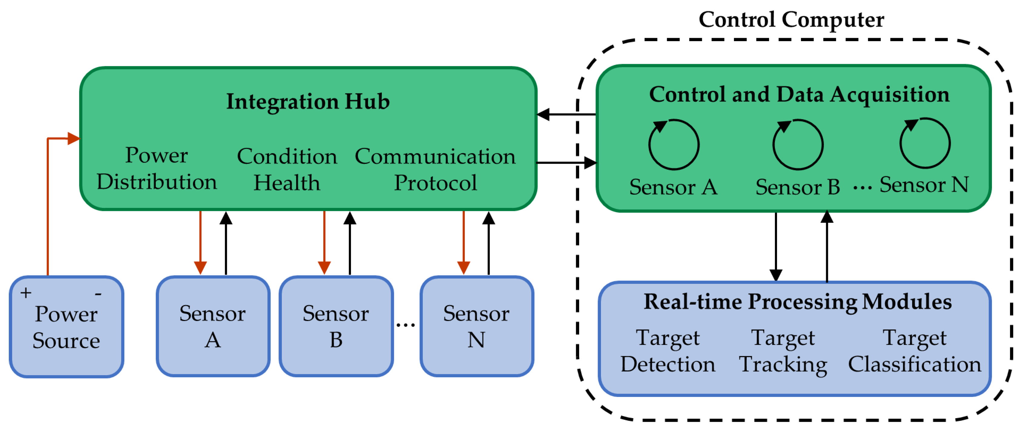
2. System Architecture

At a high level, the AMP has three subsystems: the package of integrated sensors, an external power source, and a control computer. Some elements are deployment-agnostic (e.g., integration hub), while other elements (e.g., sensors) are specific to a deployment. As shown in Figure 1, power demands and bi-directional communications for individual sensors are aggregated at an integration hub, which receives power from a single source and distributes this to several direct current (DC) buses for use by instruments. Because data rates exceed 1 Gbps and the distance between the hub and control computer can exceed 1 km (the maximum distance, limited by fiber optic signal attenuation with existing hardware, is 40 km), the backbone communication between the integrated sensors and control computer is by fiber optic media conversion. The control computer provides several functions: configuring individual sensors, holding temporary data from all sensors in memory, processing these data in real time, and archiving data when targets of interest are detected.
The following sections describe the integration hub, individual sensors, and software architecture in more detail.

2.1. Integration Hub

At the core of the AMP is the power and data integration hub. The hub aggregates data streams from connected sensors, converts these to Ethernet protocol, if necessary (e.g., serial to Ethernet conversion), and converts from copper to fiber media for transmission over an umbilical. This link is bi-directional and allows the control computer to adjust sensor configuration during deployment. The hub monitors the current draw on each output channel to detect spikes that could indicate a sensor malfunction. Similarly, the hub contains temperature and humidity sensors, as well as an inertial measurement unit. Finally, the hub generates analog trigger signals for each active sonar to prevent acoustic interference across channels (i.e., “cross-talk”).
Power supply to the hub can be at two input levels: 200–400 VDC for power transmission over a shore cable or 48 VDC for battery power proximate to the sensors. The hub uses custom electronics to distribute power to sensors with nominal inputs of 48, 24, 12, or 5 VDC. There are 10 instrument ports on the hub that can be electrically isolated (e.g., in the event of a ground fault) by double-pull/double-throw relays for power and opto-isolated communication lines. However, the hub can support more than 10 sensors by aggregating multiple sensors to a single instrument port (e.g., a hydrophone array using only one instrument port on the hub).
Key component specifications are summarized in Table A1. The power draw for these “hotel” loads is approximately 30 W. Power conversion efficiency depends on the instantaneous sensor loads and supply voltage, but has generally been above 90 %.

2.2. Mechanical Components

Considerations for mechanical integration include site, deployment, and operational constraints. Impact design factors include access to cables during assembly, sensor field of view orientation, and minimization of structural loading from hydrodynamic drag (e.g., compact form factor, fairings). The integration hub and subsystems that are not already in submersible housings (e.g., optical cameras) are contained in custom cylindrical pressure housings (depth rating of 200 m). If heat dissipation is required, the housings are anodized aluminum tube, otherwise lower-cost schedule 80 PVC is used. Housing endcaps are secured with a filament and sealed with double piston O-rings. Wherever possible, plastics (e.g., homopolymer acetal, PVC) are used to electrically isolate components and eliminate corrosion from dissimilar metal contact. Depending on the target design life of the platform, fastening hardware is selected from either all-coat mild steel, 316 stainless steel, silicon bronze, or titanium. In addition, structural components critical to the deployment and recovery operations include redundant hardware in case of unexpected corrosion.

2.3. Sensor Hardware

As summarized in Table 1, multiple sensors have been integrated with the AMP architecture, though not all of these sensors have been deployed simultaneously on a single AMP. With the exception of the optical cameras, which involved a custom solution for stereo imaging and strobe illumination, commercial instrumentation was integrated with limited modification (e.g., the Simrad WBTmini transceiver required a custom pressure housing). The fields of view for optical and acoustic instruments are shown schematically in Figure 2. The depth rating varies by sensor from a minimum of 20 m for the echosounder transducer to a maximum of 4000 m for the Tritech and Kongsberg multibeam sonars.
Some of the sensors have geometric constraints that drove design decisions. The passive acoustic sensors (fish tag receiver and hydrophones) are ideally located away from obstructions. Furthermore, maximizing the localizing hydrophone array’s baseline extends the practical bandwidth to lower frequencies and can increase location resolution and accuracy [25,26]. For stereo-optical cameras with a target range less than 10 m, baseline separation between the cameras of at least 0.4 m is recommended, as is a camera-light separation of 0.4 m to limit optical backscatter [27,28]. These requirements motivate larger physical dimensions, which conflicts with the operational challenges of working at a marine energy site that motivate the most compact arrangement possible.

2.4. Sensor Software

The AMP control software is written in LabVIEW (National Instruments) and provides users with a graphical user interface (GUI) for direct control of the AMP. The software acquires data, as well as controls the AMP’s main electronics bottle and individual sensors. The software is composed of interconnected LabVIEW “virtual instruments” (VIs), running in parallel. A core module handles communications with the integration hub to toggle power to individual sensors, observe system health sensors (e.g., current draw) and, in the event that normal thresholds are exceeded, automatically disable affected systems. This modular software structure allows a variety of real-time processing codes to be used to control data acquisition and for the sensor mix to be tailored to the requirements of a particular deployment.
Each sensor is operated by an individual VI that handles configuration (e.g., gain, range for a multibeam sonar) and parses the data stream. The specific implementation varies by sensor. Many sensor manufacturers provide application programming interfaces (APIs) for communication over TCP/IP or serial bus according to documented telemetry. Some APIs allow direct communication with an instrument (e.g., Ocean Sonics icListen HF), while others use an external application to mediate between LabVIEW and the instrument (e.g., Kongsberg M3, Simrad WBT Mini). The BlueView M900-2250 uses a .NET-based software development kit (SDK) that can be accessed directly by LabVIEW, while the Tritech Gemini 720is SDK requires an intermediate software layer in C++. Data from sensors with relatively low data rates (e.g., current profiler, optical backscatter) can be continually archived. Data from sensors with relatively high data rates (e.g., optical camera, multibeam sonar) are stored in variable-length ring buffers (typically 60 s) in the computer’s volatile memory. These ring buffers are archived when a command is generated either by a user, on a fixed duty cycle, or by a real-time data-processing module. The ring buffer structure serves three purposes: (1) when an archival command is generated, contextual data before the event is available in temporary storage; (2) processing codes do not need to operate in true “real time”, so long as they process data before they are overwritten in the ring buffer; and (3) data stored in memory can be used to establish background levels for real-time target detection. Real-time processing modules are implemented in either MATLAB (Mathworks) or Python and communicate with the core LabVIEW module via User Datagram Protocol.

2.5. Biofouling Mitigation Measures

For longer-term deployments, biofouling mitigation measures can be critical to maintaining sensor operations. The optical backscatter sensor has an integrated copper shutter with a brush wiper. Similarly, the optical cameras and illumination sources are equipped with mechanical wipers (Hydro-Wiper, Zebra-Tech, Ltd., Nelson, New Zealand) and copper face plates surrounding optical surfaces [30]. Ultraviolet (UV) lighting (AML Oceanographic, Saanichton, Canada) is used to minimize biofouling on transducers both as a precautionary measure due to uncertainties about the impact on performance and to avoid potential damage during cleaning. All biofouling control (e.g., wiper actuation) is integrated into a single, custom package that interfaces with the integration hub such as the other AMP sensors. For the most recent deployment (Section 3.4), which included both wipers and UV lighting, the wipers were actuated every 30 min and the UV lights were operated for 30 min every 60 s. Each wiper actuation draws approximately 6.5 W for 8 s and each UV light draws 2.5 W when illuminated. In addition, prior to each deployment, transducer and hydrophone elements are coated with a zinc oxide paste (40% content diaper rash cream). To reduce clean-up time following extended deployments, we have adopted the practices of wrapping housings in vinyl tape and sheathing cables with plastic “painter’s hose”. These can be easily removed (along with fouling) and disposed of at recovery.

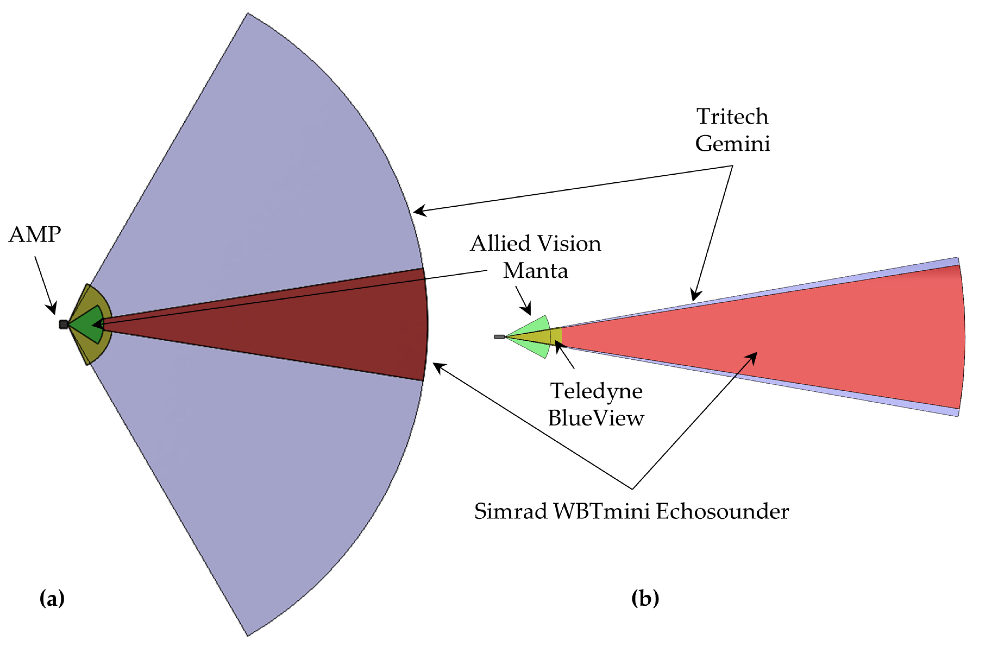
2.6. Adjustable Field of View

For initial deployments, the AMP sensor field of view was fixed. In the most recent deployment (Section 3.4), a tilt actuator (P-25, Remote Ocean Systems, San Diego, CA, USA) was integrated and allows the sensor head (instrumented with directional sensors such as the optical cameras and active sonars) to rotate through an arc of 270 ° .

3. Representative Deployments

In this section, salient details from four AMP deployments are presented in chronological order, each of which demonstrates a particular capability or contrasts modes of operation (Table 2, Figure 3). The primary objective of these deployments was to explore the general benefit of integrated instrumentation, with a secondary objective of collecting opportunistic environmental data (i.e., data that could inform future studies with specific hypotheses or permitting processes).

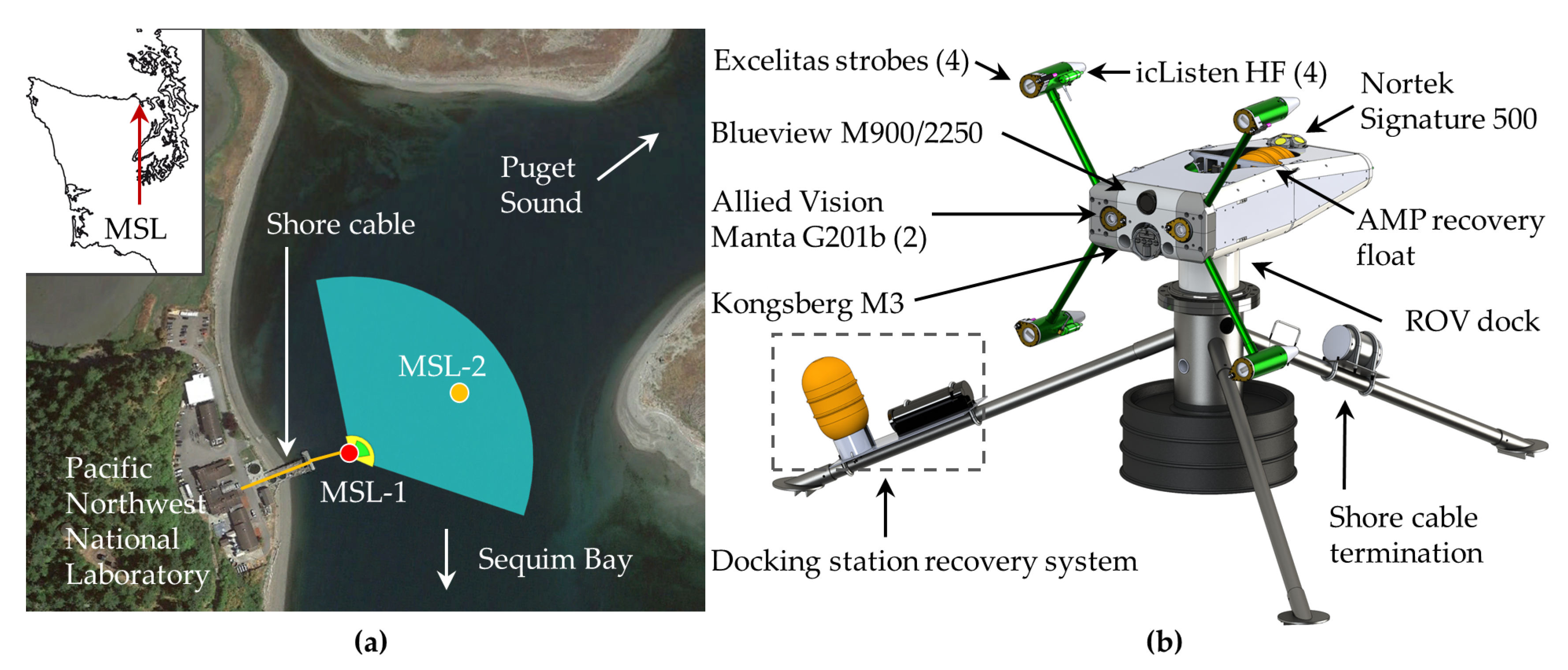
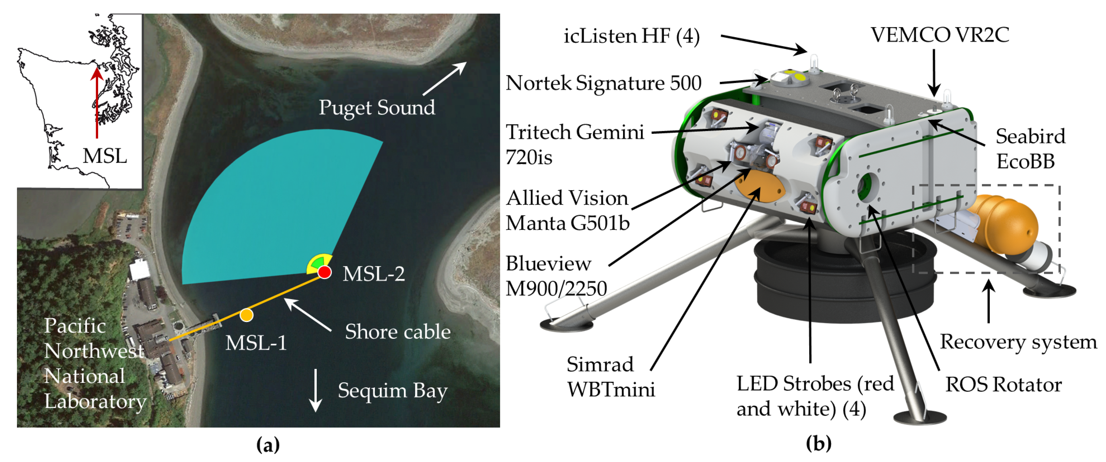
3.1. MSL-1 Demonstration

During this deployment, the AMP was operated over a cable at a marine energy demonstration site, the Pacific Northwest National Laboratory’s Marine Science Lab (PNNL MSL) in Sequim, WA, USA (Figure 4). Sensors were oriented in a horizontal plane approximately perpendicular to the direction of the tidal currents (peak velocity of ≈1.5 m/s). Prior deployments at PNNL MSL (not described) focused on hardware functionality and software development for individual sensors. During this deployment, for the first time, a real-time data-processing module on the shore computer detected and tracked targets in the multibeam sonar data streams (BlueView M900-2250 and Kongsberg M3) [19]. This module generated a data archival command when a tracked target exceeded apparent size and intensity thresholds that were manually tuned ad hoc to generate the maximum number of false positive detections that could be feasibly reviewed by the project team. Data were simultaneously collected on a sparse duty cycle to evaluate the false negative rate of the target detection and tracking module [19]. System availability (Table 2) was deemed sufficient to proceed with higher-risk, autonomous deployments.

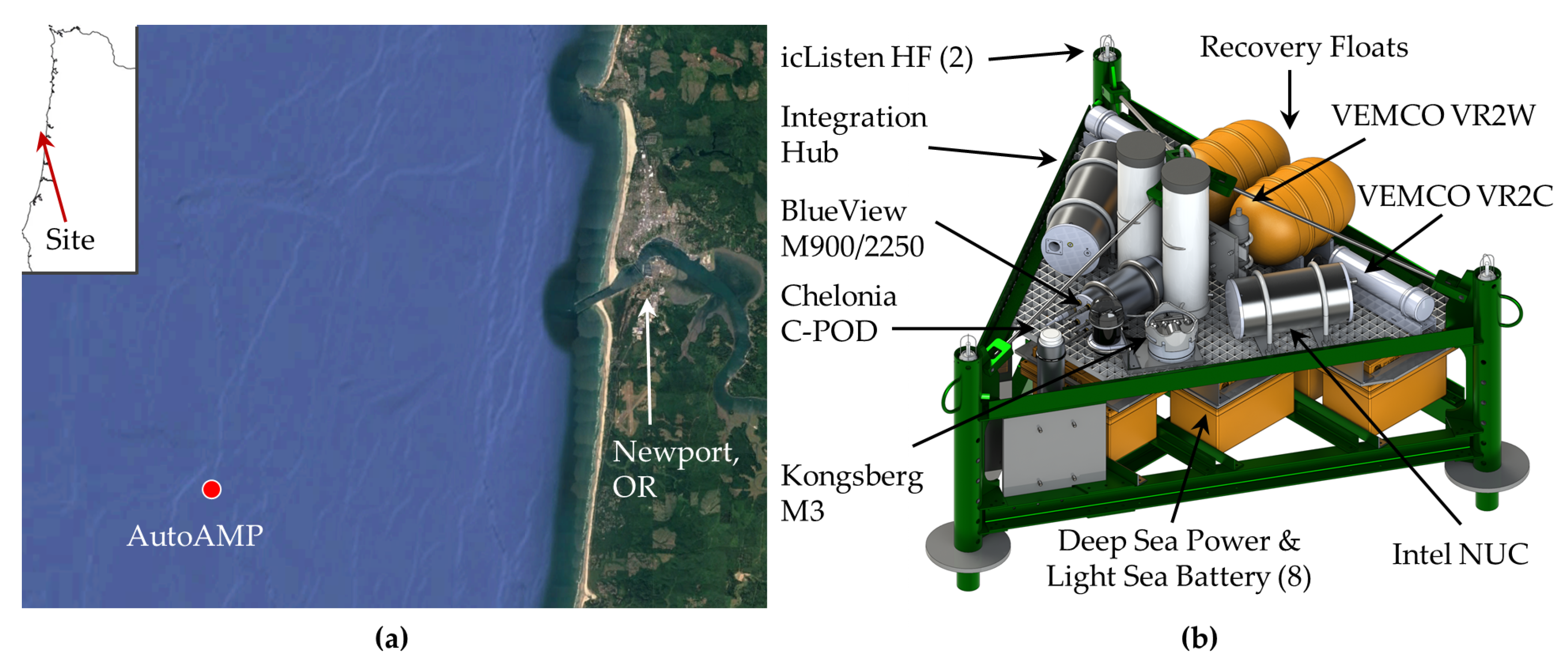
3.2. Autonomous Adaptable Monitoring Package (AutoAMP)

During this deployment, the AMP was operated autonomously using battery power in the Pacific Ocean off of Newport, OR (Figure 5). This location is under development as a grid-connected wave energy test site (PacWave South, pacwaveenergy.org) but does not yet have power or data cables back to shore. While a battery-powered system cannot meet the objectives outlined in Section 1 (i.e., continuous observation and real-time control are infeasible due to the power required), such deployments can collect useful environmental information for site development and permitting activities without incurring the expense of cable installation. Due to the water depth and moderate wave climate, the AMP only experienced significant structural loading during deployment and recovery. The battery bank (eight Sea Battery modules, Deep Sea Power & Light, San Diego, CA, USA) had a capacity of 6900 Wh and data acquisition was controlled by a compact computer (NUC NUC6i7KYK, Intel, Santa Clara, CA, USA) on the platform. This computer had sufficient processing power to record data streams on a duty cycle, but would not have been able to run target detection algorithms used during the MSL-1 deployment even if we had not been energy constrained by the batteries. The system was operated on a duty cycle by a low-power microcontroller, acquiring 120 s of data every 2 h. Prior to each acquisition sequence, 60 s were allocated to boot up and initialize and, following acquisition, up to 60 s to shut down. This duty cycle balanced available battery power and storage capacity (2 TB) for the anticipated deployment duration. In addition, the system was configured to power on and acquire data upon detection of a tagged fish. This was achieved by passing messages from a fish tag receiver (Vemco VR2C) to the microcontroller and enabling power if a tag was detected. In doing so, the AMP could gather contextual environmental information concurrent with the presence of a tagged fish. In contrast to MSL-1, the hardware frame was configured as a bottom lander with vertically oriented instrument and ballast provided by the battery bank.
This deployment did not include optical cameras due to power limitations that prevented the use of artificial lighting to illuminate the scene (a requirement for optical cameras at this depth). Furthermore, due to concerns about acoustic interference, a current profiler was not included (hardware triggering for concurrent operation of all active acoustic instruments was implemented for the MSL-2 deployment). These omissions prohibited optical review of targets or determination of target motion relative to currents.
The system operated as intended for the deployment, with the exception of two missed cycles (out of a total of 577 planned cycles) and one 24 h period early in the deployment during which sensors recorded only 20–30 s of data before shutting down. Neither of these failure modes occurred during dockside testing prior to deployment, nor could they be replicated in the lab post hoc. For each duty cycle, uptime averaged 3.3 min (out of the 4 min allocated), with a range of 2.8–3.8 min due to variations in the start-up and shut-down time on each cycle.

3.3. Wave-Powered Adaptable Monitoring Package (WAMP)

The WAMP was a first-of-a-kind integration of a sensor package with relatively high power requirements with a wave energy converter. This enabled continuous sensor operation and real-time processing, realizing many of the benefits of cabled deployments. Wave-generated power allowed us to maintain full operation of the AMP sensors for 84% of the 3.5 month deployment: an order of magnitude increase in system activity relative to the AutoAMP for a deployment more than twice as long and with significantly higher power draw (Table 2). Data were transmitted back to shore over a high-bandwidth radio frequency link (>200 Mbps, Rocket 5AC Lite, Ubiquiti Networks, New York, NY, USA) that enabled review of collected data prior to system recovery and control of the AMP software. The AMP software was configured to archive data on a duty cycle (once every hour) or when targets were detected and tracked in the multibeam sonar data, using the same real-time processing module as for MSL-1.
The WAMP was deployed at the Wave Energy Test Site (WETS) in Kaneohe, HI (Figure 6). During the deployment, the average wave climate had a significant wave height of 1.9 m and energy period of 8 s, with significant wave height increasing to 4.2 m during a storm. The WAMP was rigidly coupled to the wave energy converter (a BOLT-class Fred. Olsen Lifesaver), with the sensor head at a depth of 2 m. This depth was selected as a trade-off between high cantilever loads on the mounting structure and a desire to avoid interference in the optical and active acoustic data from air bubbles. Joslin et al. [31] presents a complete discussion of structural design, power systems integration, and system performance. While this deployment demonstrated the potential for wave-generated power to enable environmental monitoring, the primary deployment motivation was to characterize marine animal interactions with the Fred. Olsen Lifesaver. This particular wave energy converter, with an outer diameter of 16 m, was capable of generating an order of magnitude more power than required for the WAMP. Smaller wave energy converters designed to power oceanographic observations are an area of active research and development (e.g., [32]).

3.4. MSL-2 Demonstration

The final AMP deployment described here was in Sequim, WA (PNNL MSL), approximately 100 m further into the channel than the first deployment (Figure 7), with peak currents ≈2 m/s. This system relied on real-time processing modules, primarily acquiring data when targets were detected and tracked in the multibeam sonar data and, secondarily, on a sparse duty cycle. Real-time target detection and classification capabilities were demonstrated [23].

4. Results

Here, we discuss trends across the four representative deployments in Section 3 with an emphasis on practical considerations, such as biofouling and corrosion, sensor performance across environments and deployment modes, and the effectiveness of automated detection and classification algorithms that can reduce the volume of data produced by continuous observation.

4.1. Practical Considerations

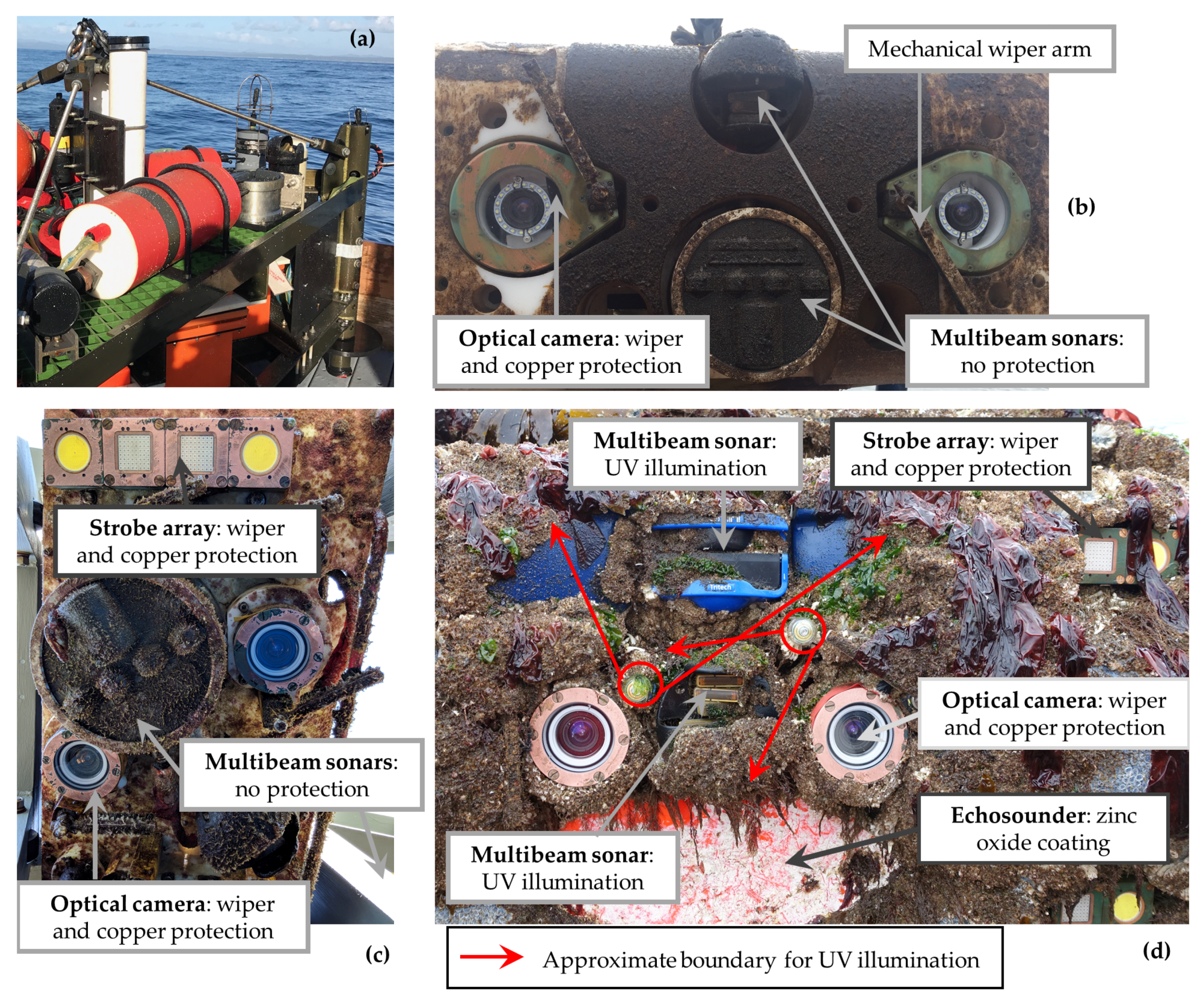
4.1.1. Biofouling and Mitigation

Figure 8 shows the condition of all four deployments at time of recovery, annotated with sensor position and protective measures. Fouling varies strongly with location, depth, duration, and season. For example, MSL-1 occurred entirely before seasonal barnacle recruitment in 2017, but MSL-2 was in the water during recruitment and was recovered a month after barnacles began to grow. An earlier deployment in 2016 was fouled similarly to MSL-2 and motivated the inclusion of UV lights in the MSL-2 build to prevent barnacle colonization of the multibeam sonar transducers. The AutoAMP had accumulated virtually no fouling at recovery and the WAMP, while in the water for longest, was less fouled than MSL-2. Consequently, depending on deployment specifics and mitigation measures, biofouling may either necessitate recovery after several months or be incidental to maintenance cycles.
In terms of mitigation measure effectiveness, mechanical wipers and copper face plates maintained high optical clarity during all deployments. UV illumination for the MSL-2 deployment partially prevented fouling on active sonars (Figure 8d), but multiple UV sources would be required to fully illuminate the transducers, as shadowed areas accumulated significant fouling. We also note that the echosounder, which was coated with zinc oxide paste prior to deployment, experienced limited fouling. Similar treatment may be effective for multibeam transducers if deployment durations are limited.
One type of “biofouling” we did not anticipate was reef effects. For the WAMP deployment, the optical field of view was often “cluttered” by reef fish (dominantly sergeant majors, Abudefduf saxatilis), as discussed in Section 4.3.2. Crabs also caused issues during two deployments. During MSL-1, a crab occupied the interior cavity of the BlueView sonar for several days and generated a large number of automatic detections that archived data without targets of interest. During the AutoAMP deployment, crabs colonized the lander and the scraping of their carapaces on the metal surfaces periodically dominated the soundscape at frequencies up to 1 kHz. Similar soundscape contributions at higher frequencies have been documented for hermit crabs on coral reefs [33].

4.1.2. Corrosion

We ensured that all systems were electrically isolated (Section 2.2), which limited instances of corrosion during all deployments. However, significant corrosion did occur at dissimilar metal interfaces on some manufacturer’s instruments, such as 316 stainless steel—titanium interfaces at bulkheads. Mild steel snap rings applied to these bulkheads were moderately effective at limiting corrosion rates, but complete mitigation would require a redesign by equipment manufacturers. we note that using zinc-alloy anodes to mitigate dissimilar metal corrosion between stainless steel and titanium is not recommended due to the large difference in anodic index [34]. A large anodic index will cause rapid wasting of the anode, such that the base metal can be unprotected for a substantial portion of a longer deployment.

4.1.3. Adjustable Field of View

While the inclusion of a tilt motor for the sensor head adds cost and complexity, our experience from MSL-2 is that these considerations are outweighed by increased functionality. First, the tilt motor allowed us to periodically look at the seabed to confirm sensor and illumination operation, as well as observe gravel and shell hash movement in high currents. Second, after deployment, the tilt motor allowed us to optimally position the active acoustic sensors to minimize interference from the water surface and seafloor. Third, when we conducted testing around the AMP with cooperative targets, we were able to orient the sensors towards the surface to determine when a vessel was directly over the platform.

4.2. Sensor Performance

4.2.1. Optical Cameras

As shown in Figure 9, optical data can help communicate findings from an acoustic image, particularly at close range where it can be difficult to classify targets using sonar [23]. Overall, optical camera imagery can be used for species-level classification, is more easily interpreted than sonar data, and is more robust to platform motion.
The effective range of optical cameras is strongly site specific. At WETS, visibility greater than 10 m was common and, in strong sunlight, the seabed was visible at a range of 30 m. In comparison, visibility at MSL was generally less than 5 m. At night, even with artificial illumination, range was reduced to a few meters at MSL and WETS. Depending on the size of marine energy converters, this range limitation can be a significant challenge for optical observations of interactions (Section 5.2).

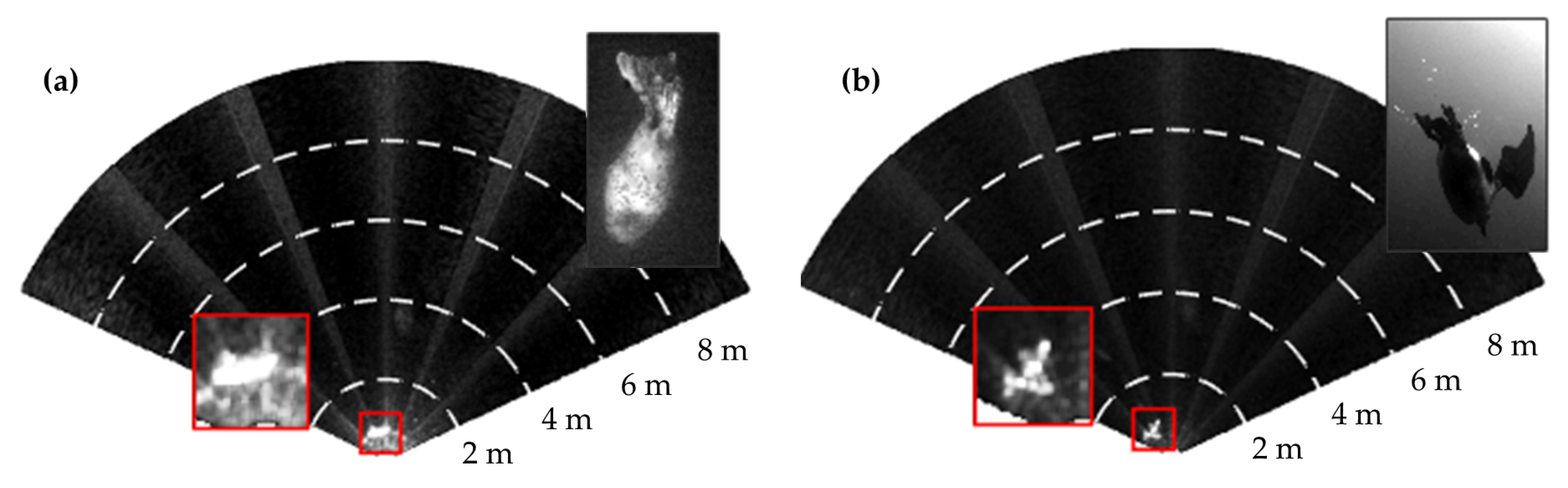
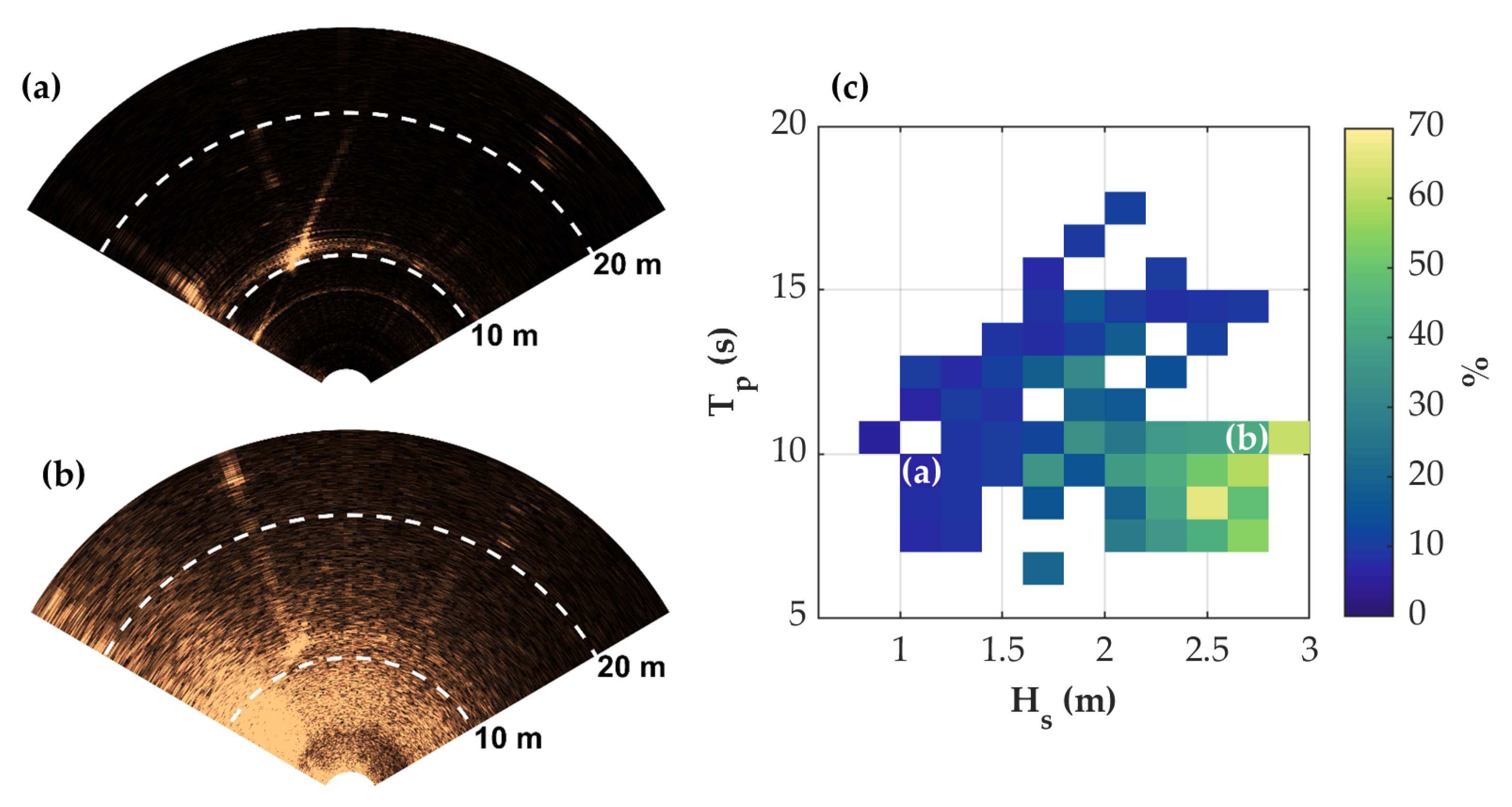
4.2.2. Multibeam Sonars

The functional range of multibeam sonars was significantly greater than the optical cameras, but subject to interference from the seafloor or water surface depending on the position of the sonar in the water column. In a horizontal configuration (MSL-1 and MSL-2), target detection became more difficult once the sonar swath intersected the water surface or seabed.
During the WAMP deployment, when the multibeam sonars were positioned near the surface and oriented at an angle downwards towards one of the mooring lines, air bubbles in the upper water column caused two issues. First, even in calm sea states, air bubbles severely reduced the range of the BlueView’s 2250 kHz transducer, requiring us to switch to the 900 kHz transducer. Second, air bubbles from breaking waves periodically obscured portions of the sonar swath (Figure 10a,b). The degree of obstruction increased in proportion to wave steepness (Figure 10c).

4.2.3. Passive Acoustics

To date, passive acoustics on the AMP have primarily provided useful diagnostic information (e.g., correlating artifacts in sonar imagery with vessel wakes). At MSL, there are few vocalizing marine mammals and while humpback whales (Megaptera novaeangliae) are seasonally abundant at WETS, none were vocalizing during the WAMP deployment.
The localizing performance of the hydrophone array was quantified using “cooperative” targets (Vemco fish tags, Ocean Sonics icTalk HF transducer). During MSL-1, this testing revealed that the AMP body (Figure 4) significantly shadowed sound propagation to some of the hydrophones, depending on source position. This contributed to the redesign of the array for MSL-2 (Figure 7), which achieved more uniform performance in cooperative target testing. Similar interference occurred for the fish tag receiver placement on the AutoAMP (Figure 5). This was corrected for MSL-2 and, during in situ tests, the receiver integrated with the AMP had a similar detection range to an autonomous fish tag receiver on a stand-alone mooring.
In general, passive-acoustic integration poses a design conflict between the need for hydrophones to be unobstructed (to avoid shadowing) and widely spaced (for accurate bearing estimation), and for instrumentation systems to be compact for ease of deployment and recovery. In addition to our experience with the AMP, in one recent tidal turbine deployment, hydrophone nodes were dispersed on a turbine’s support structure, which provided sufficient baseline separation for source localization. However, even with redundant hydrophones at each node, instrumentation failures rendered portions of the array inoperable, as the elements could not be serviced without recovering the entire turbine [35].

4.3. Automatic Target Detection and Classification

An outcome of hardware and software integration is the ability to work with multiple data streams in real time. This can enable continuous observation without accruing unmanageable volumes of data, as well as control sensors to minimize animal bias. As an example, if the AMP sensors for MSL-2 (Table 1 and Table 2 were to continuously archive data, 1.2 TB of storage would be required per day, or ≈0.5 PB of storage per year. Automatic, real-time target detection that avoids archiving “empty” data can greatly reduce these storage requirements. Further reductions are possible with real-time target classification if not all targets in the field of view are of equal interest for an environmental monitoring study. For these reasons, automatic target detection and classification were implemented in real-time for multibeam sonar data for the MSL and WAMP deployments, and in post-processing for optical camera data. In this section, we summarize these efforts and some of the operational challenges encountered in their implementation. Full details of algorithm development and validation for the multibeam sonar are provided in separate publications [19,23].

4.3.1. Multibeam Sonar

For multibeam sonar processing, we emphasize that target detection (i.e., determining that a target is present in the sonar field of view) is independent from target classification (i.e., assigning a class to a detected target). Algorithms developed to date have been primarily applied to imagery from the BlueView M900-2250, but initial explorations suggest these results are transferable to the Tritech Gemini [24] and may be similarly transferable to the Kongsberg M3.
The real-time detection module first implemented during MSL-1 triggered data archival when targets were present in the multibeam sonar data using manually tuned thresholds for apparent size and intensity. While this method produced a relatively high number of false positives (i.e., >40% of data acquisition triggers were caused by “non-biological targets”, such as sonar artifacts or high-intensity backscatter attributed to entrained air), it reduced the volume of data by an order of magnitude relative to continuous archiving [19]. To quantify detector accuracy, we reviewed nearly 1000 sequences when a data acquisition command was not generated by the detection module (e.g., no target was predicted to be present) and acquisition occurred on a regular duty cycle. Only 1% of these sequences contained a target that was not automatically detected, which is an acceptable false negative rate. We also simulated duty cycle data collection and estimated that a 5% duty cycle (45 s of data every 15 min) would be expected to capture just 6% of the automatically detected events, and less than 2% of recorded sonar sequences would contain a target of interest [19]. This means that duty cycle observation is unlikely to capture targets of interest that are infrequently present (i.e., “rare events”).
Target detection for the WAMP deployment proved more challenging because a mooring line and subsea float in the field of view created moving artifacts of comparable apparent size and intensity to biological targets of interest. This meant that target detection based on size and intensity thresholds was ineffective because thresholds that admitted biological targets would also admit most artifacts. we attempted to compensate for this by masking regions of the swath, but because the sonar motion was independent of float motion, the artifacts varied in apparent size, position, and intensity. Preliminary investigation suggests that the algorithm used for optical camera processing (Section 4.3.2) may be an effective alternative target detector for sonar imagery acquired from stationary and moving platforms and will be tested in future AMP deployments.
This detection step also facilitated the training of machine learning algorithms for automatic target classification. By reviewing only sequences with detected targets, relatively limited human effort was required to annotate the data to train machine learning algorithms for classification, as compared to annotating continuously acquired data. In post-processing, a random forest algorithm discriminated between biological (e.g., seals, schools of fish, and diving birds) and non-biological targets with a recall rate (true positive classifications relative to actual members of the target class) of 0.97 and precision (true positive classifications relative to all positive classifications) of 0.60 [23]. Furthermore, this algorithm was able to distinguish targets associated with seals, birds, and fish schools with recall rates of 0.91, 0.88, and 0.91, respectively. The inputs to the classification model are an optimized set of hand-engineered features that describe statistical attributes of all detections making up a target’s track (e.g., 75th percentile major axis length) and environmental covariates (e.g., time of day) [23].
These training data were used to evaluate classification model performance and implement real-time, automatic classification for MSL-2 [23]. Initially, when the classification model used for MSL-2 was trained only using data collected at MSL-1, the model performed relatively poorly—less than 50% of biological targets were correctly classified (recall rates for biological target classes <0.5) [23]. This reduction in performance relative to recall rates of ≈0.9 in post-processing of MSL-1 data is attributable to differences in site characteristics and biological activity between MSL-1 and MSL-2. Specifically, the stronger currents at MSL-2 produced more non-biological targets associated with entrained air. Similarly, at MSL-1, temporal patterns of biological activity were, in retrospect, affected by artificial lighting on shore. Specifically, harbor seals appeared primarily at night during MSL-1, likely because they were using the dock lighting to forage, but appeared throughout the day during MSL-2. However, after a relatively small volume of new training data from MSL-2 was added to the classification model, performance improved significantly, with greater than 70% of biological targets correctly classified (recall rates for biological classes >0.7). The site-specific nature of biological classification algorithms trained with smaller volumes of data agrees with the findings of Rosa et al. [36] for classification of birds in radar data.

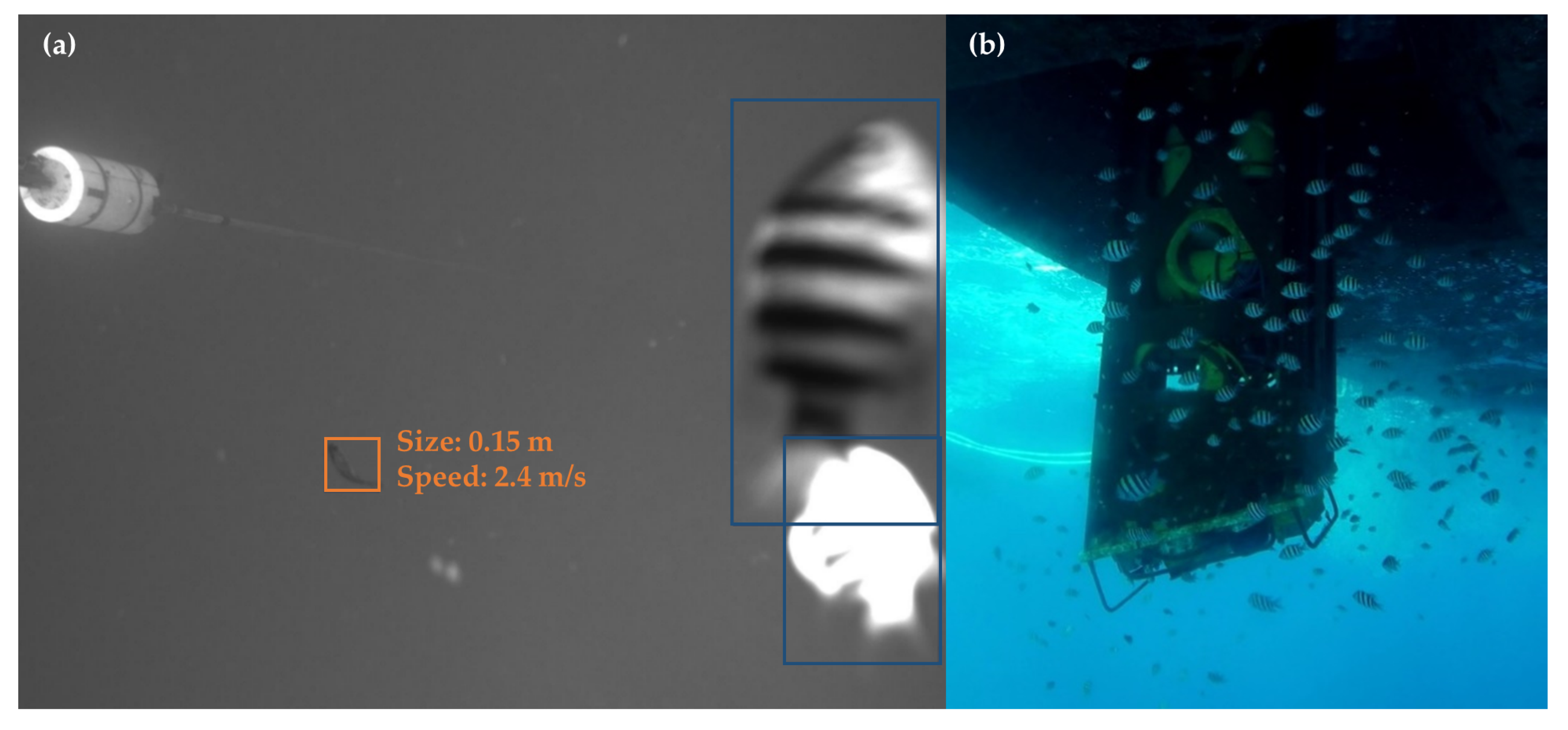
4.3.2. Optical Cameras

Optical processing methods implemented to date involve concurrent target detection and classification using the YOLO (You Only Look Once) deep-learning algorithm [37,38]. Our motivation for using this algorithm stems from prior demonstrated success using this approach to detect fish in optical imagery [39]. The YOLO algorithm produces both class identification and bounding box target location in candidate images. Using a binary (i.e., biological vs. non-biological) YOLO model with annotated imagery from MSL and WETS, we were able to obtain recall of 0.83 and precision of 0.96 in WETS data when predicted bounding boxes had a 0.4 overlap divided by area (i.e., Intersection over Union) threshold measured against ground truth data. Additionally, a two-class model to distinguish reef fish (e.g., sergeant majors) from non-reef fish (e.g., a tuna-like species) produced a recall of 0.71 and precision of 0.96, averaged over the two classes, using the same evaluation criteria. To develop this model, we employed an iterative process of training the model with limited data, then curating the output and retraining with the expanded image set. At the end of this iterative process, we had curated 17,481 training images from MSL (primarily without targets present) and 2469 training images from WETS. In addition, automatic stereo image processing shows promise in extracting target size and speed (Figure 11). To estimate target size, we: (1) extract YOLO-produced bounding boxes; (2) predict corresponding targets between stereo images by searching for a similarly sized bounding box along a rectified image epipolar line [40], and; (3) triangulate the 3D bounding box corner positions using the calibrated stereo extrinsics [41]. Similarly, to estimate target speed, we search temporally identified YOLO bounding boxes for similarly sized-targets, and estimate speed as distance traveled divided by time between captured frames. As target motion is not constrained, correspondence between temporal frames cannot be limited to an epipolar line search, which makes accurate temporal correspondence more difficult. As such, speed estimates have a relatively high implicit uncertainty, particularly when multiple targets are present.

5. Discussion

5.1. Evidenced Requirements for Integrated Instrumentation

Our experiences with AMP deployments evidence several requirements for effective use of integrated instrumentation systems at marine energy sites. First, to observe “rare events” without producing unmanageable volumes of data, it is essential to provide sufficient power for continuous sensor operation and real-time processing [19], whether by cable or in situ energy harvesting. When limited by batteries, as for the AutoAMP (Section 3.2), the type of sensors that can be supported and the maximum allowable duty cycle are relatively low, given power requirements for sensing and real-time processing (Table 1 and Table 2). As another example, the initial deployments of the FLOWBEC platform relied on battery power [12], which limited deployments to 14 days, restricted the sensor suite, did not allow real time data processing, and devoted the majority of the platform structure to battery storage.
Second, deployment outcomes are improved by providing connectivity for continuous data transmission. By reviewing data products in near real-time, problems can be rapidly identified and corrected, rather than only becoming apparent during a post-deployment analysis phase. For example, during the WAMP deployment, we initially enabled the 2250 kHz head on the BlueView sonar based on our favorable experience during MSL-1 and AutoAMP deployments. If we had not been able to review data during the WAMP deployment, we would not have discovered that air bubbles rendered it mostly ineffective until after recovery. The ability to access and review data at the time of collection also minimizes the risk of inadvertently accruing and curating large volumes of irrelevant data, as well as providing the opportunity for iterative model training (c.f., Section 4.3.2).
Third, integrated instrumentation should be designed to be maintained at intervals no longer than six months. Although no critical sensor failures have occurred during AMP deployments, problems such as corrosion at dissimilar metal interfaces on manufacturer-supplied equipment have been developed over our longest deployments. While it is likely is that engineering solutions and biofouling mitigation measures can extend endurance beyond what we have demonstrated, and we believe it is critical to design integrated instrumentation systems for recovery and repair.

5.2. Operational Concepts for Integrated Instrumentation

When integrated instrumentation is used to monitor marine energy installations, there are multiple deployment options, all of which involve trade-offs. The first two evidenced requirements for integrated instrumentation (power availability and data connectivity) are most easily satisfied by a cabled connection to terrestrial facilities. Consequently, satisfying the third evidenced requirement (maintenance intervention) suggests operational strategies that share several features with maintenance of grid-connected marine energy converters (MECs). Specifically, if the instrumentation is connected to a cable, then either the cable needs to be recovered along with the instrumentation or a “docking” capability is required to connect to and disconnect from the cable. Similarly, there are two approaches to securing the instrumentation package: integrating it into the structure of a MEC or using a separate structure.
Operational concepts for integrated instrumentation can be classified by three attributes:
  • Securement strategy: integrated with a MEC and independent structure;
  • Position in the water column: surface, mid-water, and seabed; and
  • Marine energy resource: waves, oscillating tidal currents, and continuous ocean currents.
The securement strategy restricts the range of stand-off distances between the integrated instrumentation package and a MEC. Specifically, if the securement strategy is to integrate the instrumentation with a MEC, then the maximum stand-off distance between the sensors and components of interest on the MEC is likely on the order of 10 m, given the size of existing MECs. Conversely, if an independent structure is used, then the minimum stand-off distance is likely on the order of 10 m due to space requirements for marine operations to install and maintain the independent structure, regardless of the position of the structure in the water column.
If a monitoring objective is to observe interactions between marine animals and a MEC, then integrating instrumentation with a MEC is preferred. Our experience suggests that automatic classification of targets in multibeam sonars becomes increasingly difficult at ranges greater than 10 m. Similarly, outside of tropical waters, the range of optical cameras is generally less than 10 m. Given this, the field of view will likely only include a portion of most utility-scale MECs. While sonar deployment from an independent platform at greater stand-off distance may place an entire MEC within the field of view [12], this arrangement significantly reduces image resolution, such that detection and classification of smaller targets would be more difficult. In addition, moored, independent platforms add data processing complexity due to relative motion and operational complexity due to the need to control position and orientation during deployment.
The position in the water column imposes several restrictions for docking instrumentation to a cabled node or recovering the cable. For surface deployments, docking or cable recovery is relatively straightforward as the “docking” connection and cable handling can occur out of the water (c.f., the WAMP). For subsurface deployments, docking and cable recovery have different challenges. For docking, wet-mate power and data connections with sufficient bandwidth for integrated instrumentation can be costly and the mating process often requires relatively fine alignment and moderate engagement force. For example, a Teledyne ODI NRH connector can only tolerate a linear offset <4 mm and an angular offset <10 ° during mating and requires >500 N engagement force. Early AMP developments included successful demonstration of a wet-mate system using an inspection-class ROV (Figure 12), and docking station [42,43], but the complexity, risk, and cost motivated a cable recovery strategy for MSL-1 and MSL-2. For cable recovery, the connectors can be dry-mate, with substantially lower cost, but this requires a customized approach to controlling package orientation during redeployment, maintenance operations put the cable and instrumentation system at risk, and steps must be taken to avoid collision or entanglement with a nearby MEC. For the MSL deployments, the water was shallow enough for us to coarsely orient the AMP with guy lines as it was deployed, but this would not be feasible in deeper water.
General operation and maintenance considerations for each resource type, depending on position in the water column and securement strategy, are summarized in Table 3. In doing so, we have assumed a nominal “mid-water” depth of 25 m and a nominal seabed depth of 50 m for tidal and wave energy, and a nominal seabed depth of 300 m for ocean current energy [5]. Each combination is assigned a qualitative difficulty denoted by the color shading, which progresses from relative ease (no shading) to operations that are infeasible with existing technology (dark blue). There are several apparent trends. First, there are no scenarios in which both operation and maintenance can be achieved with relative ease. Second, there is a trade-off between the simplicity of operations and the simplicity of maintenance. Third, wave energy installations are the most straightforward to instrument, followed by tidal currents. Ocean currents present several significant technical challenges for sub-surface instrumentation maintenance. Overall, operations and maintenance considerations should be central to instrumentation development and, optimally, a “co-design” exercise between those engaged in environmental monitoring and those deploying MECs.
We note that these capability concepts can be facilitated by complimentary technology developments. For example, non-contact power and data transfer solutions are under development and could substantially simplify the complexity of docking operations by eliminating physical connectors. Similarly, reducing the sensor payload would reduce the size of instrumentation packages and facilitate deployment and recovery. This requires environmental studies to identify the minimum sensor set needed to answer a specific question, which will likely only become apparent as questions are answered using a broader set of sensors.

5.3. Cost-Benefit of Integration

Instrument integration into a compact package is a difficult task. The successful demonstrations of AMP systems have had to overcome interference between active sonars, electrical noise on shared power busses3, Ethernet traffic conflicts, and the need to rewrite instrument control and data acquisition software. This raises the question of whether integration is worthwhile.
One way to think about integration is in terms of “phases”, with each phase enabling a fundamental capability. we define Phase 1 integration as providing power and data connectivity to a range of sensors through a common backbone. This enables hardware deployment as a single, integrated package. Phase 2 integration involves a common software architecture for sensor control and data acquisition. This enables synchronous and duty-cycled data acquisition. Phase 3 integration builds on this by evaluating data streams in real time to make decisions about data acquisition and sensor control.
In our opinion, there are clear benefits to each phase, but the cost-benefit trade-off may not always favor integration. Phase 1 integration dramatically simplifies maintenance. Furthermore, if a MEC-integrated strategy is employed (Section 5.2), the interface specification for an integrated package on a turbine or wave energy converter can be as simple as a bolt pattern and a cable for power and data. Distributing instrumentation across a wider area can have benefits for passive acoustic tracking [35] and stand-off distance, but significantly increases integration cost and precludes the evidenced requirement for independent maintenance of sub-surface instrumentation. Phase 1 integration also allows multiple fields of view to be observed from a single platform and make concurrent observations of marine animals with different sensing modalities (Figure 9 and Figure 13). Overall, our experience is that the benefits of Phase 1 integration outweigh the costs.
Phase 2 integration requires setting aside much of the software written by manufacturers and rebuilding functionality using manufacturer-provided software development kits or communication protocol specifications. it would be difficult to overstate the difficulty we encountered in this process. While Phase 2 integration does simplify duty-cycle acquisition and guarantees that all acquisition occurs on the same master clock (though does not preclude master clock drift without a cabled connection or GPS), it could be argued that the cost to achieve this is disproportionate to the benefits. In general, outside of stereo image processing, precise timing is not critical—knowing that an animal was present with sub-second accuracy is not likely much more informative than knowing it was present within a 10 s period.
However, Phase 2 integration is a precursor to Phase 3 integration, which, in our experience, is the only way to address the prioritized monitoring requirements laid out in Section 1 and resolve the implicit conflict between the priorities. In addition to reducing data volumes from continuous observation (Section 4.3), when data are evaluated in real time, the risk of behavioral bias associated with some observations can be substantially mitigated. For example, decisions can be made about enabling artificial illumination for optical acquisition based on target proximity, as determined from a multibeam sonar. Phase 3 integration also provides real-time classification models access to environmental correlates, such as water current velocity and direction. In our opinion, the greatest benefits from Phase 3 integration are the ones that have yet to be realized, as the marine biology community should be able to use integrated architectures to conduct new types of targeted observation (e.g., long-term predator-prey interaction studies). This could also enable machine learning already employed in oceanographic studies (e.g., [44]) to be used in real time. Similarly, integrated instrumentation has clear applications to port and harbor security and, perhaps, other applications yet to be considered.

6. Conclusions

In this paper, we presented details of the AMP system, described system and sensor performance across four, multi-month deployments, and demonstrated the feasibility of integrated instrumentation in cabled and autonomous modes of operation. Our experience with AMP development is that an integrated instrumentation system can provide a reliable and cost-effective solution to environmental monitoring at marine energy sites. However, we emphasize that significant non-recurring engineering effort is required to develop such systems and, consequently, this should not be undertaken lightly. System design must consider the specific environmental questions to be studied, as well as considerations for operation and maintenance in marine energy environments (e.g., biofouling mitigation, deployment strategy). Full integration of hardware and software allows rare events to be observed, minimizes the volume of data not containing interactions of interest, avoids biasing animal behavior while sensing, and enables tractable maintenance strategies. Concurrent developments in marine energy and integration instrumentation have implications beyond our ability to monitor environmental interactions for utility-scale marine energy converters. As demonstrated by the WAMP deployment, coupling integrated instrumentation with small wave energy converters or current turbines can enable observations similar to a cabled observatory—but without the cable. While hardware and software challenges undoubtedly remain, integrated instrumentation systems, such as the AMP, have reached a point of maturity where they can effectively contribute to the body of knowledge about the environmental effects of marine energy.

Author Contributions

Conceptualization, B.P., J.J., A.S., and E.C.; methodology, B.P., J.J., A.S., E.C., P.M., and C.B.; software, E.C., P.M., and M.S.; formal analysis, E.C. and M.S.; investigation, J.J., P.M., P.G., E.C., and M.S.; data curation, E.C., P.M., and M.S.; writing—original draft preparation, B.P., J.J., E.C., P.G., P.M., M.S.; writing—review and editing, C.B. and A.S.; visualization, P.G., E.C., M.S., B.P., and J.J.; supervision, B.P. and A.S.; project administration, B.P. and A.S.; funding acquisition, B.P. and A.S. All authors have read and agreed to the published version of the manuscript.

Funding

This material is based upon work supported by the U.S. Department of Energy’s Office of Energy Efficiency and Renewable Energy (EERE) under the Water Power Technologies Office award numbers DE-EE0006788 and DE-EE0007827. The WAMP deployment was supported by the U.S. Department of Defense’s Naval Facilities Engineering Command (N00024-08-D-6323 Task Order No. 16). E.C. was supported by a National Science Foundation Graduate Research Fellowship.

Acknowledgments

The authors would like to acknowledge the technical contributions of the following individuals and organizations: University of Washington: Haleh Bahadori, Eric Boget, Robert Cavagnaro, Corey Crisp, Jesse Dosher, Bryan Ford, Craig Hill, John Horne, Trina Litchendorf, Ben Maurer, Darshan Mehta, Jessica Noe, Andy Reay-Ellers, Chris Siani, Zack Tully, and Benjamin Williamson; Oregon State University: Sarah Henkel, Geoff Hollinger, and the crew of R/V Pacific Storm; Pacific Northwest National Laboratory: Kate Hall, Genevra Harker-Klimes, Kailan Mackereth, Margaret Pinza, Shari Matzner, Sue Southard, Garrett Staines, and John Vavrinec; University of Hawai’i: Patrick Cross and Andrew Druetzler; Sea Engineering, Inc.: Patrick Anderson and Andrew Rocheleau; and Fred. Olsen Renewables: Even Hjetland.

Conflicts of Interest

J.J. is commercializing the AMP technology through MarineSitu, Inc. The funders had no role in the design of the study; in the collection, analyses, or interpretation of data; in the writing of the manuscript, or in the decision to publish the results.

Abbreviations

The following abbreviations are used in this manuscript:
3DThree-dimensional
AMPAdaptable Monitoring Package
APIApplication Programming Interface
AutoAMPAutonomous AMP
DCDirect Current
MSLMarine Science Laboratory
PNNLPacific Northwest National Laboratory
ROVRemotely Operated Vehicle
SDKSoftware Development Kit
WAMPWave-powered AMP
WETSWave Energy Test Site

Appendix A

Table A1. Key integration hub components.
Component FunctionManufacturerModel(s)
DC-DC power conversionVicor, MA, USADCM 200-400 VDC, DCM 48-48 VDC,
Mini 48-24 VDC, Mini 48-12 VDC
Media conversionMoxa, TaiwanEDS-G516E Series
Serial to Ethernet conversionMoxa, TaiwanNPort-5200 Series
Table A2. Sensor configurations for data rates shown in Table 1.
SensorSetting
Nortek Signature 5000.5 m resolution and range of 8 m (MSL-1 and MSL-2)
BlueView M900-2250Compressed JPEG image format in polar coordinates (range and
transducer agnostic)
Tritech GeminiCompressed JPEG image format in Cartesian coordinates (range and
transducer agnostic)
Kongsberg M3ASCII format with arc resolution of 0.95 ° (15 ° vertical beam angle), range
resolution of 0.03 m, and range of 50 m (MSL-1 and WAMP)
Simrad WBTminiSingle operational channel logging to a range of 75 m with the smallest file
configuration (narrowband operation with high data compression). The data rate
is sensitive to signal types (broadband vs. narrowband), data compression
options, and logging range [29]. The use of broadband signals with minimal
compression increases the data rate by approximately two orders of magnitude.
Allied Vision
Manta G507b
Compressed JPEG from 8-bit, monochrome image (5 Mpx)

References

  1. Copping, A.; Sather, N.; Hanna, L.; Whiting, J.; Zydlewski, G.; Staines, G.; Gill, A.; Hutchison, I.; O’Hagan, A.; Simas, T.; et al. Annex IV 2016 State of the Science Report: Environmental Effects of Marine Renewable Energy Development around the World; Technical Report; International Energy Agency Ocean Energy Systems: Lisbon, Portugal, 2016.
  2. Copping, A.; Hemery, L. OES-Environmental 2020 State of the Science Report: Environmental Effects of Marine Renewable Energy Development Around the World; Technical Report; International Energy Agency Ocean Energy Systems: Lisbon, Portugal, 2020.
  3. Gunn, K.; Stock-Williams, C. Quantifying the global wave power resource. Renew. Energy 2012, 44, 296–304. [Google Scholar] [CrossRef]
  4. Falnes, J.; Kurniawan, A. Ocean Waves and Oscillating Systems: Linear Interactions Including Wave-Energy Extraction; Cambridge University Press: Cambridge, UK, 2020; Volume 8. [Google Scholar]
  5. Barnier, B.; Domina, A.; Gulev, S.; Molines, J.M.; Maitre, T.; Penduff, T.; Le Sommer, J.; Brasseur, P.; Brodeau, L.; Colombo, P. Modelling the impact of flow-driven turbine power plants on great wind-driven ocean currents and the assessment of their energy potential. Nat. Energy 2020, 5, 240–249. [Google Scholar] [CrossRef]
  6. Karsten, R.; Swan, A.; Culina, J. Assessment of arrays of in-stream tidal turbines in the Bay of Fundy. Philos. Trans. R. Soc. A Math. Phys. Eng. Sci. 2013, 371, 20120189. [Google Scholar] [CrossRef] [PubMed] [Green Version]
  7. Polagye, B.; Thomson, J. Tidal energy resource characterization: Methodology and field study in Admiralty Inlet, Puget Sound, WA (USA). Proc. Inst. Mech. Eng. Part A J. Power Energy 2013, 227, 352–367. [Google Scholar] [CrossRef]
  8. Lewis, M.; Neill, S.; Robins, P.; Hashemi, M. Resource assessment for future generations of tidal-stream energy arrays. Energy 2015, 83, 403–415. [Google Scholar] [CrossRef] [Green Version]
  9. Bassett, C.; Thomson, J.; Polagye, B. Sediment-generated noise and bed stress in a tidal channel. J. Geophys. Res. Ocean. 2013, 118, 2249–2265. [Google Scholar] [CrossRef]
  10. Polagye, B.; Copping, A.; Suryan, R.; Kramer, S.; Brown-Saracino, J.; Smith, C. Instrumentation for Monitoring around Marine Renewable Energy Converters: Workshop Final Report; Technical Report PNNL-23100; Pacific Northwest National Laboratory: Seattle, WA, USA, 2014.
  11. Hasselman, D.; Barclay, D.; Cavagnaro, R.; Chandler, C.; Cotter, E.; Gillespie, D.; Hastie, G.; Horne, J.; Joslin, J.; Long, C.; et al. Environmental Monitoring Technologies and Techniques for Detecting Interactions of Marine Animals with Marine Renewable Energy Devices. In OES-Environmental 2020 State of the Science Report: Environmental Effects of Marine Renewable Energy Development Around the World; Copping, A.E., Hemery, L.G., Eds.; International Energy Agency Ocean Energy Systems: Lisbon, Portugal, 2020; pp. 177–212. [Google Scholar]
  12. Williamson, B.J.; Blondel, P.; Armstrong, E.; Bell, P.S.; Hall, C.; Waggitt, J.J.; Scott, B.E. A self-contained subsea platform for acoustic monitoring of the environment around Marine Renewable Energy Devices–Field deployments at wave and tidal energy sites in Orkney, Scotland. IEEE J. Ocean. Eng. 2015, 41, 67–81. [Google Scholar]
  13. Hastie, G.D.; Gillespie, D.M.; Gordon, J.C.; Macaulay, J.D.; McConnell, B.J.; Sparling, C.E. Tracking technologies for quantifying marine mammal interactions with tidal turbines: Pitfalls and possibilities. In Marine Renewable Energy Technology and Environmental Interactions; Springer: Berlin, Germany, 2014; pp. 127–139. [Google Scholar]
  14. Cotter, E.; Murphy, P.; Bassett, C.; Williamson, B.; Polagye, B. Acoustic characterization of sensors used for marine environmental monitoring. Mar. Pollut. Bull. 2019, 144, 205–215. [Google Scholar] [CrossRef]
  15. Marchesan, M.; Spoto, M.; Verginella, L.; Ferrero, E.A. Behavioural effects of artificial light on fish species of commercial interest. Fish. Res. 2005, 73, 171–185. [Google Scholar] [CrossRef]
  16. Widder, E.; Robison, B.; Reisenbichler, K.; Haddock, S. Using red light for in situ observations of deep-sea fishes. Deep. Sea Res. Part I Oceanogr. Res. Pap. 2005, 52, 2077–2085. [Google Scholar] [CrossRef]
  17. Wiesebron, L.E.; Horne, J.K.; Hendrix, A.N. Characterizing biological impacts at marine renewable energy sites. Int. J. Mar. Energy 2016, 14, 27–40. [Google Scholar] [CrossRef]
  18. Wilding, T.A.; Gill, A.B.; Boon, A.; Sheehan, E.; Dauvin, J.C.; Pezy, J.P.; O’beirn, F.; Janas, U.; Rostin, L.; De Mesel, I. Turning off the DRIP (‘Data-rich, information-poor’)—Rationalising monitoring with a focus on marine renewable energy developments and the benthos. Renew. Sustain. Energy Rev. 2017, 74, 848–859. [Google Scholar] [CrossRef]
  19. Cotter, E.; Murphy, P.; Polagye, B. Benchmarking sensor fusion capabilities of an integrated instrumentation package. Int. J. Mar. Energy 2017, 20, 64–79. [Google Scholar] [CrossRef]
  20. Cowles, T.; Delaney, J.; Orcutt, J.; Weller, R. The ocean observatories initiative: Sustained ocean observing across a range of spatial scales. Mar. Technol. Soc. J. 2010, 44, 54–64. [Google Scholar] [CrossRef]
  21. Hayes, S.; Mangum, L.; Picaut, J.; Sumi, A.; Takeuchi, K. TOGA-TAO: A moored array for real-time measurements in the tropical Pacific Ocean. Bull. Am. Meteorol. Soc. 1991, 72, 339–347. [Google Scholar] [CrossRef] [Green Version]
  22. Kohler, P.C.; LeBlanc, L.; Elliott, J. SCOOP-NDBC’s new ocean observing system. In Proceedings of the IEEE OCEANS 2015-MTS/IEEE, Washington, DC, USA, 19–22 October 2015; pp. 1–5. [Google Scholar]
  23. Cotter, E.; Polagye, B. Automatic classification of biological targets in a tidal channel using a multibeam sonar. J. Atmos. Ocean. Technol. 2020. [Google Scholar] [CrossRef]
  24. Cotter, E.; Polagye, B. Biological detection and classification capabilities of two multibeam sonars. Limnol. Oceanogr. Methods. In revision.
  25. Watkins, W.A.; Schevill, W.E. Sound source location by arrival-times on a non-rigid three-dimensional hydrophone array. Deep. Sea Res. Oceanogr. Abstr. 1972, 19, 691–706. [Google Scholar] [CrossRef]
  26. Wahlberg, M.; Møhl, B.; Teglberg Madsen, P. Estimating source position accuracy of a large-aperture hydrophone array for bioacoustics. J. Acoust. Soc. Am. 2001, 109, 397–406. [Google Scholar] [CrossRef] [Green Version]
  27. Jaffe, J.S. Underwater optical imaging: The design of optimal systems. Oceanography 1988, 1, 40–41. [Google Scholar] [CrossRef] [Green Version]
  28. Joslin, J.; Polagye, B.; Parker-Stetter, S. Development of a stereo-optical camera system for monitoring tidal turbines. J. Appl. Remote. Sens. 2014, 8, 083633. [Google Scholar] [CrossRef]
  29. Demer, D.; Andersen, L.; Bassett, C.; Berger, L.; Chu, D.; Condiotty, J.; Cutter, G. Evaluation of a Wideband Echosounder for Fisheries and Marine Ecosystem Science; Technical Report 336; ICES Cooperative Research Report; ICES: Copenhagen, Denmark, 2017. [Google Scholar]
  30. Joslin, J.; Polagye, B. Demonstration of biofouling mitigation methods for long-term deployments of optical cameras. Mar. Technol. Soc. J. 2015, 49, 88–96. [Google Scholar] [CrossRef] [Green Version]
  31. Joslin, J.B.; Cotter, E.D.; Murphy, P.G.; Gibbs, P.J.; Cavagnaro, R.J.; Crisp, C.R.; Stewart, A.R.; Polagye, B.; Cross, P.S.; Hjetland, E.; et al. The wave-powered adaptable monitoring package: Hardware design, installation, and deployment. In Proceedings of the 13th European Wave and Tidal Energy Conference, Napoli, Italy, 1–6 September 2019. [Google Scholar]
  32. Mundon, T.R. Performance evaluation and analysis of a micro-scale wave energy system. In Proceedings of the 13th European Wave and Tidal Energy Conference, Napoli, Italy, 1–6 September 2019; pp. 1686-1–1686-8. [Google Scholar]
  33. Freeman, S.E.; Rohwer, F.L.; D’Spain, G.L.; Friedlander, A.M.; Gregg, A.K.; Sandin, S.A.; Buckingham, M.J. The origins of ambient biological sound from coral reef ecosystems in the Line Islands archipelago. J. Acoust. Soc. Am. 2014, 135, 1775–1788. [Google Scholar] [CrossRef]
  34. Roberge, P.R. Handbook of Corrosion Engineering; McGraw-Hill: New York, NY, USA, 2000. [Google Scholar]
  35. Malinka, C.E.; Gillespie, D.M.; Macaulay, J.D.; Joy, R.; Sparling, C.E. First in situ passive acoustic monitoring for marine mammals during operation of a tidal turbine in Ramsey Sound, Wales. Mar. Ecol. Prog. Ser. 2018, 590, 247–266. [Google Scholar] [CrossRef] [Green Version]
  36. D. Rosa, I.M.; Marques, A.T.; Palminha, G.; Costa, H.; Mascarenhas, M.; Fonseca, C.; Bernardino, J. Classification success of six machine learning algorithms in radar ornithology. Ibis 2016, 158, 28–42. [Google Scholar] [CrossRef]
  37. Redmon, J.; Divvala, S.; Girshick, R.; Farhadi, A. You only look once: Unified, real-time object detection. In Proceedings of the IEEE Conference on Computer Vision and Pattern Recognition, Las Vegas, NV, USA, 27–30 June 2016; pp. 779–788. [Google Scholar]
  38. Redmon, J.; Farhadi, A. Yolov3: An incremental improvement. arXiv 2018, arXiv:1804.02767. [Google Scholar]
  39. Xu, W.; Matzner, S. Underwater fish detection using deep learning for water power applications. In Proceedings of the IEEE International Conference on Computational Science and Computational Intelligence (CSCI), Las Vegas, NV, USA, 13–15 December 2018; pp. 313–318. [Google Scholar]
  40. Papadimitriou, D.V.; Dennis, T.J. Epipolar line estimation and rectification for stereo image pairs. IEEE Trans. Image Process. 1996, 5, 672–676. [Google Scholar] [CrossRef]
  41. Hartley, R.I.; Sturm, P. Triangulation. Comput. Vis. Image Underst. 1997, 68, 146–157. [Google Scholar] [CrossRef]
  42. Rush, B.; Joslin, J.; Stewart, A.; Polagye, B. Development of an Adaptable Monitoring Package for marine renewable energy projects Part I: Conceptual design and operation. In Proceedings of the 2nd Marine Energy Technology Symposium, Seattle, WA, USA, 15–18 April 2014. [Google Scholar]
  43. Joslin, J.; Polagye, B.; Rush, B.; Stewart, A. Development of an adaptable monitoring package for marine renewable energy projects Part II: Hydrodynamic performance. In Proceedings of the 2nd Marine Energy Technology Symposium, Seattle, WA, USA, 15–18 April 2014. [Google Scholar]
  44. Sheehan, E.V.; Bridger, D.; Nancollas, S.J.; Pittman, S.J. PelagiCam: A novel underwater imaging system with computer vision for semi-automated monitoring of mobile marine fauna at offshore structures. Environ. Monit. Assess. 2020, 192, 11. [Google Scholar] [CrossRef]
1.
Specialized hydrophones that continuously monitor for unique identifiers that are acoustically broadcast by tags attached to or implanted in fish.
2.
This is common practice for some autonomous sensors. For example, one passive acoustic sensor for quantifying cetacean presence-absence, the C-POD-F (Chelonia Ltd., Cornwall, UK) continuously monitors frequencies between 20 kHz and 160 kHz by sampling at 1 MHz, but processes the data in real time to identify candidate echolocation clicks and archives only statistical information about those clicks for post-recovery analysis. Similar principles apply to fish tag receivers. The Vemco VR2W (Innovasea, Bainbridge Island, WA, USA) continuously monitors for tags with a transmit frequency of 69 kHz, but only stores the time and unique tag identifier of decoded detections.
3.
As a specific example, the load on the primary Vicor DC-DC power converters in the integration hub (Table A1) had a measureable effect on the noise floor for the WBTmini echosounder, even though the power busses were nominally independent. In passive mode, the WBTmini noise floor varied by more 14 dB, based on which instruments were energized, including mechanical wipers and UV lights. This change in noise floor has the effect of reducing the echosounder’s operational range and signal-to-noise ratio.
Figure 1. AMP architecture schematic. Black arrows denote flows of data, red arrows denote flows of power, and shading differentiates between deployment-specific (blue) and deployment-agnostic (green) components.
Jmse 08 00553 g001
Figure 2. AMP sensor field of view for a horizontally oriented deployment showing the AMP body to scale for (a) top-view and (b) side-view with the Manta optical cameras to 8 m (nominal range), BlueView sonar to 10 m, Gemini sonar to 80 m, and Simrad echosounder to 80 m.
Jmse 08 00553 g002
Figure 3. AMP configurations from select deployments: (a) MSL-1, (b) AutoAMP, (c) WAMP, and (d) MSL-2. Top row: Photographs of AMP configurations. Middle row: constant-scale profile view of instrumentation and core platform elements (excludes mounting structures). Bottom row: constant-scale view of primary sensor head.
Jmse 08 00553 g003
Figure 4. MSL-1 AMP deployment showing (a) site layout with MSL-2 location noted and (b) AMP and docking station lander. The AMP control computer was located on shore.
Jmse 08 00553 g004
Figure 5. AutoAMP deployment showing (a) site layout and (b) AMP lander.
Jmse 08 00553 g005
Figure 6. WAMP deployment showing (a) site layout, (b) AMP configuration, excluding power take-off modules on the Fred. Olsen Lifesaver, and (c) AMP sensors.
Jmse 08 00553 g006
Figure 7. MSL-2 deployment showing (a) site layout and (b) AMP configuration.
Jmse 08 00553 g007
Figure 8. AMP biofouling at recovery for the four deployment case studies: (a) AutoAMP: 44 day at 70 m—negligible fouling, (b) MSL-1: 77 days at 8 m depth— limited fouling, (c) WAMP: >200 days (system in water longer than operated) at 2 m depth—moderate fouling, and (d) MSL-2: 118 days at 7 m depth— heavy fouling.
Jmse 08 00553 g008
Figure 9. Comparison of optical and active acoustic (BlueView multibeam sonar, 2250 kHz) representations of a (a) seal and (b) diving bird from MSL-1. Adapted from [19].
Jmse 08 00553 g009
Figure 10. Kongsberg M3 multibeam sonar during WAMP deployment with (a) low and (b) high levels of bubble intrusion. (c) Average percentage of the sonar image (Kongsberg M3) that was obscured by bubbles as a function of the significant wave height ( H s ) and peak wave period ( T p ), based on an analysis of 147 sonar sequences. Sea states for (a) and (b) are annotated. The obstructed region was determined by applying a threshold to the image, and finding the region of the image above the threshold connected to the surface (e.g., left-hand side of (a)). Morphological filters (dilation and fill) were then applied to reduce the effects of noise.
Jmse 08 00553 g010
Figure 11. (a) Automated size and speed estimation from WAMP deployment imagery. Size is reported as the diagonal length of predicted 3D bounding box. The reef fish on the right margin have been automatically identified as not of interest. (b) Representative reef clutter observed by external camera during WAMP inspection.
Jmse 08 00553 g011
Figure 12. ROV deployable version of AMP tested prior to MSL-1. The ROV delivered the AMP to a pre-placed, cabled docking station (frame in Figure 4), engaged a wet-mate power and fiber connector (Teledyne ODI NRH), and then returned to the surface.
Jmse 08 00553 g012
Figure 13. (a) Three fish automatically detected by the YOLO optical algorithm (outlined in magenta) also apparent in (b) BlueView multibeam sonar data (manually outlined in magenta).
Jmse 08 00553 g013
Table 1. AMP sensors. For some sensors, data rates depend on settings, as summarized in Table A2.
CategorySensorInput
Voltage
[VDC]
Maximum Acquisition
Rate (Stand-Alone /
AMP Synchronized)
[Hz]
Power Requirement
(Synchronized
Acquisition Rate)
[W]
Data Rate
(Single
Instrument)
Comms
Protocol
Field
of View
Maximum
Range [m]
Acoustic Doppler
current profiler
Nortek Signature
500 (Norway)
12–488/523<3 × 10 4 RS-232 or
Ethernet
2.9 ° beam
width
70
Multibeam sonarBlueView M900-2250
(U.S.)
12–4815/1019.2<0.1
MB/frame
Ethernet130 × 20 °
swath
200 kHz: 10
900 kHz: 100
Tritech Gemini (U.K.)19–7297/1916–27<0.1
MB/frame
Ethernet130 × 20 °
swath
120
Kongsberg M3
(Norway)
12–3640/1024.0< 1.3
MB/frame
Ethernet120 ° ×
3,7,15, or 30 °
swath
150
EchosounderSimrad WBTmini
(w/ 38/200 kHz combi-
transducer) (Norway)
12–1638 kHz: <4/<4
200 kHz: >10/10
Passive: > 10 /10
38 kHz: 6
200 kHz: 3
Passive: 2
0.002
MB/ping
Ethernet18 ° beam
width
38 kHz: >500
200 kHz:
>100
Passive acousticVemco VR2C (Canada)10–32N/A0.2< 0.001
MB/message
RS-232Omni-
directional
N/A
icListen HF
(Ocean Sonics, Canada)
24512,000/512,0003.63 × 10 6
MB/sample
Ethernet
Optical
backscatter
SeaBird ecoBB
(650 nm) (U.S.)
7–158<13 × 10 6
MB/sample
RS-232N/AN/A
Optical cameraAllied Vision Manta
G201b & G507b
(Canada)
1223/104.8<0.3
MB/frame
Ethernet65 × 56 ° 0–30
Xenon strobeExcelitas MVS-500
(U.S.)
1214/1063.6N/AN/AN/AN/A
LED strobe
(red/white)
Custom LED Arrays48Continuous/
camera-limited
49N/AN/AN/AN/A
Table 2. Adaptable Monitoring Package deployment summary. “System availability” is % of time available for sensing and “system activity” is % of time actively sensing. Power requirements are only for offshore components.
DeploymentMSL-1AutoAMPWAMPMSL-2
LocationSequim Bay, WA, USA (MSL)
48 ° 4.76’ N, 123 ° 2.68’ W
Newport, OR, USA (PacWave)
44 ° 32.86’ N, 124 ° 13.78’ W
Kaneohe, HI, USA (WETS)
21 ° 27.94’ N, 157 ° 45.04’ W
Sequim Bay, WA, USA (MSL)
48 ° 4.79’ N, 123 ° 2.60’ W
Dates (duration)10 January–28 March 2017
(77 days)
15 August–29 September 2017
(44 days)
15 October 2018–28 January 2019
(105 days)
30 January–28 May 2019
(118 days)
System availability/activity≈90%/90%>99%/1.7%84%/84%96%/96%
Deployment typeCabled bottom landerAutonomous bottom landerAutonomous surface platformCabled bottom lander
Distance to shore0.1 km12.5 km1.5 km0.2 km
Water depth8 m (MLLW)70 m30 m7 m (MLLW)
Dominant environmentTidal currentWaveWaveTidal current
Power requirement373 W161 W696 W240 W
Power sourceShore cableBattery bank
(6900 Wh capacity)
Battery-backed wave
energy converter
Shore cable
Real-time processingMultibeam sonar
triggered acquisition
Multibeam sonar
triggered acquisition
Multibeam sonar
triggered acquisition
and classification
Primary sensor orientationAcross-channel, fixedUpward-looking, fixedDownward-looking, fixedAcross-channel, variable tilt
Biofouling mitigationCamera and strobe wipersCamera and strobe wipersCamera and strobe wipers
UV lights for sonars
Optical sensors
CamerasAllied Vision Manta G-201bAllied Vision Manta G-507bAllied Vision Manta G-507b
IlluminationExcelitas MVS-5000Custom white and red LEDsCustom white and red LEDs
Optical backscatterSeabird ecoBB
Passive acoustic sensors
HydrophoneOceanSonics icListen HF (4)OceanSonics icListen HF (3)OceanSonics icListen HF (2)OceanSonics icListen HF (4)
Fish tag receiverVemco VR2CVemco VR2C
Active acoustic sensors
Multibeam sonarsBlueView M900-2250
Kongsberg M3
BlueView M900-2250
Kongsberg M3
BlueView M900-2250
Kongsberg M3
BlueView M900-2250
Tritech Gemini 720is
EchosounderSimrad WBTmini
Acoustic Doppler current profilerNortek Signature 500Nortek Signature 500
Table 3. Generalized operation and maintenance considerations wave wave, tidal and ocean current systems. Color progression from light to dark denotes difficulty. For waves, if water depth decreases (50 m nominal), wave orbital velocities are appreciable over relatively more of the water column. For oscillatory tidal currents, if water depth decreases (50 m nominal), currents near the seabed and at mid-water converge towards surface values. For continuous ocean currents, the region of significant currents extends to >50 m depth.
OperationsMaintenance
EnvironmentInstrument Location Integrated with MECIndependent Platform
Surface (<2 m)• High structural loads on sensors
• Significant platform motion possible
• Air bubbles occlude field of view
• Air-side access to sensors• Air-side access to cable
WavesMid-water (25 m)• Moderate structural loads and
limited platform motion
• ROV or diver
intervention
• Heavy lift capacity to raise
platform and cable to surface
(more significant mooring and
anchoring requirement than
platform on seabed)
Seabed (50 m)• Low structural loads and no
platform motion
• ROV intervention• Moderate lift capacity to raise
platform and cable to surface
Surface (<2 m)• Highest structural loads:
strongest currents at surface
Air bubbles occlude field of view
• Air-side access to sensors• Air-side access to cable
Oscillatory
Tidal Currents
Mid-water (<2 m)• Moderate structural loads:
currents decrease with depth
• ROV or diver intervention
during slack water
• Heavy lift capacity to raise platform
and cable to surface during slack water
Seabed (50 m)• Lowest structural loads:
currents at minimum near seabed
• ROV intervention
during slack water
• Heavy lift capacity to raise platform
and cable to surface during slack water
Surface (<2 m)• Highest structural loads:
strongest currents at surface
• Air bubbles occlude field of view
• Air-side access to sensors• Air-side access to cable
Continuous
Ocean Currents
Upper water
column (50 m)
• Moderate structural loads:
currents decrease with depth
• High-thrust ROV required• Heavy lift capacity vessel
with high thrust required
Seabed (300 m)• Stand-off between sensors and
turbine exceeds sensor range
• ROV with launch
and recovery system to overcome
drag in upper water column
• Heavy lift capacity vessel
with high thrust required

