Design of the Depth Controller for a Floating Ocean Seismograph

Abstract

Floating ocean seismograph (FOS) is a vertical underwater vehicle used to detect ocean earthquakes by observing P waves at teleseismic distances in the oceans. With the requirements of rising to the surface and transmitting data to the satellite in real time and diving to the desired depth and recording signals, the depth control of FOS needs to be zero overshoot and accurate with fast response. So far, it remains challenging to implement such depth control due to the variation of buoyancy caused by the seawater density varying with the depth. The deeper the water is, the greater the impacts on buoyancy are. To tackle it, a fuzzy sliding mode controller considering the influence of seawater density change is proposed and simulated in MATLAB/SIMULINK based on the variable buoyancy system and state space function of FOS. Compared with proportional-integral-derivative (PID) controller, fuzzy PID controller and sliding mode controller, the simulation results indicate that the proposed controller shows its superiority regardless of the disturbing force. Its advantages include smaller steady-state error, faster response time, smaller system chatter, and well robustness. This proves that the designed fuzzy sliding mode controller is able to meet the working requirements and thus, lays a foundation for FOS application.

1. Introduction

With the development of human science and technology, the exploration process of the ocean is gradually expanding to include deeper depths and more remote locations, and the research on the structure and the internal dynamics of the deep earth has become critical. The detection of ocean seismic waves serves to notice the thermal or compositional anomalies in Earth’s mantle and core [1,2,3], and to image the mantle plume [4]. However, the lack of the ocean seismic stations poorly constrained the unveiling of the earth structure due to its 70% coverage by water. The formation of the ocean seismograph network is of great significance and value to scientific research [5], and floating ocean seismographs (FOS) can exactly realize such value [6]. It is a vertical underwater vehicle used to observe P waves (primary waves, the first signal from an earthquake) in ocean earthquakes [7,8].

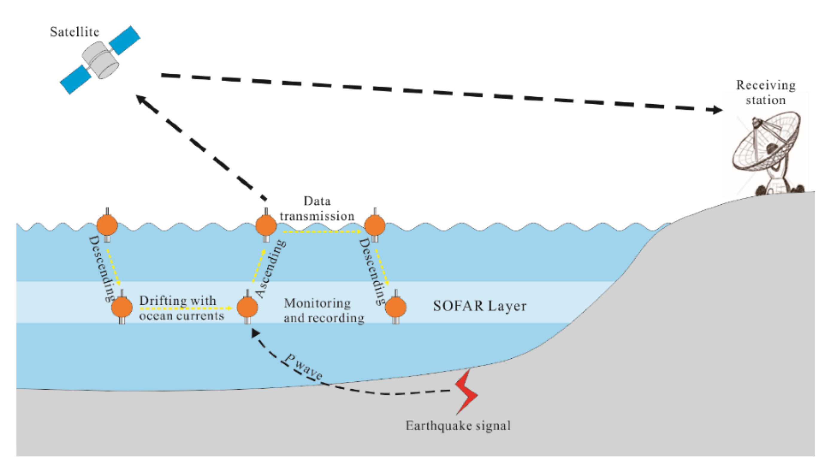
Unlike the conventional stationary land seismic stations and submersible ocean bottom seismographs (OBS), FOS is suspended in the water column during its work time after diving to the desired parking depth set in the SOFAR (sound fixing and ranging channel) layer shown in Figure 1 [1]. It is used to detect seismic waves and record seismic signals while drifting with ocean currents. It rises to the surface and transmits the data to the satellite when P waves are detected or the memory card is full. Then, it dives and another cycle starts. After a number of FOSs are densely deployed, they drift along with ocean currents with no need of a horizontal thruster or any other form of power engine and spread over the oceanic area, forming a global scope of seismic monitoring network [9]. Its global positioning system (GPS) makes the real-time transmission of data more convenient [2]. Its buoyancy control system controls its dive to the preset parking depth and float to the surface to communicate with satellite.

In the working process, FOS fluctuates with flows and currents at the water depth of 1000 m and may be subject to disturbance forces from flows, currents, sea animals, and other uncertain objects. This would affect the real depth of FOS resulting in lower measurement accuracy and even lead to bottoming out with unsatisfactory depth control. It is also known that as the depth of the FOS increases, its buoyancy varies due to the density change of seawater. While the variable buoyancy system (VBS) is used to adjust FOS drainage volume to change its buoyancy, mainly depending on its design is difficult to achieve the accurate depth control. Furthermore, to reduce the impact caused by the disturbing forces, the response performance of FOS under the disturbing forces should also be critical and be verified, as well. Therefore, to tackle the abovementioned challenges, this paper mainly proposes the design of a depth controller for FOS with fast response, zero overshoot, nearly no steady-state error, and high robustness, so that when FOS detects a seismic wave, it could respond accurately, rising to the surface and sending the data signal to satellite, and then quickly diving to the desired parking depth to resume the detection work without accidental bottoming damage. In addition, precise depth position can keep different FOSs at different depths so that they would not collide with each other in the future network control research.

At present, the existing basic control methods mainly include proportional–integral–derivative (PID) control [10], sliding mode control (SMC) [11], neural network control [12], predictive control [13], and fuzzy logic control (FLC) [14,15]. Their advantages and disadvantages are as shown in

Table 1. Advantages and disadvantages of different basic control methods.

Types		Advantages	Disadvantages
Type	Acronym
Proportional–integral–derivative	PID	Easy to implement and maintain	Mainly used for linear time invariant systems
Sliding mode control	SMC	Used for nonlinear systems	Cause actuator tremors, energy waste, and error proneness
Neural network control	NNC	Convergence to a precise model	Need longer training time and slower learning rate to get accurate model
Predictive control	PC	Good performance, strong robustness, low requirements for model accuracy	Heavy calculations, not suitable for fast time-varying systems
Fuzzy logic control	FLC	Simple control structure, efficient design, good robustness, strong anti-interference ability, no need for precise models	Lower accuracy and worse quality with simple fuzzy information, have steady-state errors

[16].

With the consideration that FOS requires long-term steady work under water and the movement of diving and surfacing to transmit signals cannot be too slow, neural network control and predictive control are not considered because they need a long time to train and calculate. The PID control method is widely used in marine industrial products because of its simple structure and easy operation [17,18], the fuzzy logic control method is renowned for its simplicity, robustness, and anti-interference ability [14,19], and sliding mode control is useful for nonlinear system despite its tendency to cause “tremor” (small, rapid fluctuations in position). Two of these three control methods could be incorporated to control nonlinear systems such as FOS, and such controllers are mainly fuzzy PID controller (F-PID) [20,21] and fuzzy sliding mode controller (F-SMC) [22,23]. To some extent, the fuzzy logic method can improve the weak points of PID control and sliding mode control, but we do not know which is better. To deal with the problem that which one of the controllers is the most suitable for the FOS depth control, different controllers should be designed and analyzed. In addition, the controller to be designed for FOS thereupon is required to be able to achieve the following four goals:

• Satisfy the depth control requirements, especially the ability to maintain position at a parking depth.
• Control FOS with sufficient stability, shorter adjustment time, smaller overshoot, and smaller steady-state error approaching zero while hovering in the sea.
• Have better dynamic characteristics compared with a traditional PID controller and a sliding mode controller (fuzzy logic control has certain steady-state error, so it is not taken into consideration).
• Have good anti-interference ability and robustness.

After a brief introduction, this paper is organized as follows. Section 2 analyzes the forces that FOS is subject to and derives its dynamic model as the controller design basis with the consideration of the influence of seawater density change on the buoyancy. Section 3 describes the design of different controllers for FOS depth control, including PID controller, fuzzy PID controller, sliding mode controller, and fuzzy sliding mode controller. In Section 4, the simulation comparisons and the analysis results are elaborated and conclusions are presented in Section 5.

2. Dynamic Models

Dynamic models are used to describe the regularity of changes in the system variables over time. In the modeling, the FOS needs to maintain its working depth of 1000 m in the water column, despite buoyancy changes due to seawater density variations, which has certain impacts on FOS when considering its diving and surfacing movement control. In this section, the structure of FOS seismograph was illustrated first and then its subjected forces were analyzed in which the hydrodynamic equation was established and the transfer function of depth to the vertical force were derived.

2.1. Coordinate Systems and Forces

FOS is mainly composed of glass shell, protective housing, iridium, acoustics module, conductivity-temperature-density (CTD), micro control panel, battery pack, VBS, and oil bladder. Its outside view is shown in Figure 2, in which the protective shell at two ends are open and the inner glass float is sealed with the vacuum sealing method. In addition, the devices, such as iridium and acoustics module, outside the glass float are relatively small compared to the glass float, and their volume could be therefore negligible in the forces analysis. In the calculation, FOS is assumed to be spherical, and its vertical plane motion coordinate system is shown in Figure 3. The axis is right-handed. The general coordinate system (E-ξηζ) is fixed to the earth, and the local coordinate system (G-xyz) is fixed to the FOS. The coordinate variables of FOS in its local coordinate system are listed in

Table 2. Variables of FOS in its local coordinate system.

Degree of Freedom	Motion	Forces/Moments	Linear Velocity/Angular Velocity	Positions/Angles
1	Surge	X (N)	u (m/s)	x (m)
2	Sway	Y (N)	v (m/s)	y (m)
3	Heave	Z (N)	w (m/s)	z (m)
4	Roll	K (N·m)	p (rad/s)	φ (rad)
5	Pitch	M (N·m)	q (rad/s)	θ (rad)
6	Yaw	N (N·m)	r (rad/s)	ψ (rad)

.

FOS is mainly subject to two static forces, i.e., buoyancy and its own gravity. The gravity here is taken as the total displacement of FOS in water, denoted by W. Additionally, the total buoyancy B here includes the full drainage volume buoyancy of FOS B₀, the changes of buoyancy caused by the variance of seawater density B_ρ, and the buoyancy provided by the variable buoyancy system F_VBS, as shown below:

$$B=B_0+B_{\rho }+F_{VBS}$$

(1)

Here, the buoyancy variation B_ρ is given by [24]:

$$B_{\rho }=\left(\rho \left(\zeta \right)-{\rho }_0\right)g\nabla$$

(2)

and the density ρ(ζ) is substituted by potential density as shown in Equation (3):

$$\rho \left(\zeta \right)=\sigma \left(\zeta \right)+1000{ \mathrm{kg}/\mathrm{m}}^3$$

(3)

where ρ(ζ) is the density function varying with the depth (the data of conditional density σ(ζ) came from South China Sea observations in 2012) and could be expressed as Equation (4) by data fitting shown in Figure 4; ζ is the depth from sea surface in the general coordinate system; ρ₀ is the sea surface density;$\nabla$ is the full drainage volume of FOS.

$$\rho (\zeta )=\{\begin{array}{ll}1020.56{ \mathrm{kg}/\mathrm{m}}^3& 0<\zeta <66.37 \mathrm{m}\\ \left(26.13e^{4.674\times {10}^{-5}\zeta }-11.36e^{-0.01052\zeta }+1000\right){ \mathrm{kg}/\mathrm{m}}^3& \zeta \ge 66.37 \mathrm{m}\end{array}$$

(4)

Accordingly, the variation of buoyancy caused by change of sea density B_ρ can be described as:

$$B_{\rho }=\{\begin{array}{ll}0& 0<\zeta <66.37 \mathrm{m}\\ \left(\rho \left(\zeta \right)-1020.56{ \mathrm{kg}/\mathrm{m}}^3\right)g\nabla & \zeta \ge 66.37 \mathrm{m}\end{array}$$

(5)

In addition, the buoyancy provided by the variable buoyancy system F_VBS can be expressed as:

$$F_{VBS}={\displaystyle {\int }_0^{t_1}\rho \left(\zeta \right)g{q}_{1}dt}-{\displaystyle {\int }_0^{t_2}\rho \left(\zeta \right)g{q}_{2}dt}$$

(6)

where q₁ is the volume flow rate while pumping oil from the bladder to the tank and q₂ is the volume flow rate while pumping oil in the opposite direction, and therefore these two parts cannot coexist. The values of t₁ and t₂ depend on the maximum buoyancy adjustment volume and volume flow rate of VBS.

When balancing counterweights, the gravity W is equal to the full drainage volume buoyancy B₀. Therefore, the residual static load of FOS △P can be obtained:

$$\Delta P=W-B=W-\left(B_0+B_{\rho }-F_{VBS}\right)=F_{VBS}-B_{\rho }$$

(7)

When △P > 0, FOS sinks; when △P < 0, FOS rises up; when △P = 0, FOS is in buoyancy equilibrium.

2.2. Dynamic Models

For depth control of FOS, its six degree of freedom hydrodynamic equation should be established. The well-known hydrodynamic equation [25] can be simplified as equation (8) for FOS [26] with assumptions and specific simplifications as shown below:

• Only the motion of FOS in the vertical plane is considered due to the particularity of movement of the ocean current. Then, the movement state variables in Table 2 can be simplified as u, w, and q, namely the horizontal speed, the vertical speed, and the angular speed around the y-axis, respectively. In addition, the value of sway, pitch, and yaw is zero v = p = r = 0.
• Higher-order damping, second-order terms in u and q are neglected in the motion of FOS. The horizontal speed, the angular speed around the y-axis, the horizontal acceleration, and the angular acceleration around the y-axis are assumed as zero for convenience, that is $u=q=\dot{u}=\dot{q}=0$.
• Buoyancy equal to weight (B = W) at the initial time. Two centers of gravity and buoyancy coincide with each other. Only the disturbance force in z-direction d is considered.

  $$\left(m-Z_{\dot{w}}\right)\dot{w}-Z_{w}w=Z+d$$

  (8)

  where m is mass of FOS; w is vertical speed; $\dot{w}$ is vertical accelerate; $Z_{\dot{w}}$ denoting partial derivative of vertical force with respect to vertical acceleration is approximately the additional mass of a ball, and its formula is shown in Equation (9); Z_w denoting partial derivative of vertical force with respect to vertical speed is calculated as Equation (10) according to the ITTC nondimensional physical quantity definition [27]; Z is the vertical force, and Z = △P; d is a sinusoidal disturbance force.

  $$Z_{\dot{w}}=-\frac{1}{2}\rho \cdot \frac{4}{3}\pi R^3=-\frac{2}{3}\rho \pi R^3$$

  (9)

  $$Z_w=\frac{1}{2}\rho {\left(2R\right)}^{2}U{Z^{\prime }}_w=2\rho R^{2}U{Z^{\prime }}_w$$

  (10)

In the assumption, the value of roll, pitch, and yaw is zero, so z = ζ and the variable ζ in Equations (2)–(6) can be replaced by z. Additionally, because the derivative of depth to time is equal to the vertical velocity $\dot{z}=w$, Equation (8) can be transformed as:

$$\ddot{z}=\frac{Z_w}{m-Z_{\dot{w}}}\dot{z}+\frac{1}{m-Z_{\dot{w}}}\left(F_{VBS}-B_{\rho }+d\right)$$

(11)

Therefore, the state-space equation is given by:

$$\left[\begin{array}{c}\dot{z}\\ \ddot{z}\end{array}\right]=\left[\begin{array}{cc}0& 1\\ 0& \frac{Z_w}{m-Z_{\dot{w}}}\end{array}\right]\left[\begin{array}{c}z\\ \dot{z}\end{array}\right]+\left[\begin{array}{c}0\\ \frac{1}{m-Z_{\dot{w}}}\end{array}\right]\left(F_{VBS}-B_{\rho }+d\right)$$

(12)

In Equations (9)–(10), the density ρ is approximately constant for convenience of calculation. According to the hydrodynamic coefficients of round disc underwater vehicles and ellipsoidal underwater vehicles [28,29], the hydrodynamic coefficient of this spherical FOS is estimated as Z’_w = -0.4. In addition, the numerical values of the major parameters in the calculation are listed in

Table 3. The major parameters in the calculation.

Parameters	Numeric Values	Physical Significances
ρ	1025 kg/m3	Density of sea water
m	43.20 kg	Mass of FOS
R	0.216 m	Radius of floating ocean seismograph
U	0.8 m/s	Freestream velocity
V	1.5 L	Maximum buoyancy adjustment volume
q1, q2	1.5×10-4 m3/s	Volume flowrate of VBS

.

3. Depth Controller Design

3.1. Depth Control Principle

The depth control of FOS is realized by a variable buoyancy system and a depth controller, and the control block diagram thereof is shown in Figure 5. In the diagram, the input of the system is the desired depth z_d, and the inputs of the depth controller are the depth error e and the depth error change rate $\dot{e}$ of FOS. The output of the depth controller is the expected buoyancy B_exp after the adjustment, and the system output is the actual depth z of FOS derived from the variable buoyancy system and FOS dynamic system function. The variable buoyancy system is an actuator for FOS. The depth sensor serves as a feedback for measuring the depth, and the controller continuously adjusts the variable buoyancy system according to the feedback information to reach the target depth. At the meantime, the seawater density at actual depth is fed back to the controller in real time, which allows the more accurate buoyancy adjustment.

The expression equation of the depth error e is as follows:

$$e=z_{\mathrm{d}}-z$$

(13)

Different depth controllers are proposed in Section 3.2–Section 3.5, including PID controller, fuzzy PID controller, sliding mode controller, and fuzzy sliding mode controller. The PID controller and sliding mode controller are enhanced into fuzzy PID controller and fuzzy sliding mode controller, respectively. Their design and analysis are as follows.

3.2. PID Controller

The block diagram of PID controller is shown in Figure 6. The control input of this controller is merely the depth deviation e. The control output of the PID controller is the expected buoyancy B_exp given by Equation (14):

$$B_{\exp }=K_{\mathrm{P}1}+K_{\mathrm{I}1}{\displaystyle \int e\mathrm{d}t}+K_{\mathrm{D}1}\frac{\mathrm{d}e}{\mathrm{d}t}+B_{\rho }$$

(14)

where K_P1, K_I1, and K_D1 are proportional, integral, and differential coefficients, respectively.

3.3. Fuzzy PID Controller (F-PID)

To enhance the PID controller, the fuzzy logic method is used to allow time-variable tuning of proportional, integral, and differential coefficients, which is fuzzy PID controller. The block diagram of the fuzzy PID controller is as shown in Figure 7 [16,30], in which the controller parameters K_P, K_I, and K_D can be calculated as:

$$\{\begin{array}{c}{K}_{\mathrm{P}}=K_{\mathrm{P}0}+\alpha \Delta K_{\mathrm{P}}\\ K_{\mathrm{I}}=K_{\mathrm{I}0}+\beta \Delta K_{\mathrm{I}}\\ K_{\mathrm{D}}=K_{\mathrm{D}0}+\gamma \Delta K_{\mathrm{D}}\end{array}$$

(15)

where K_P0, K_I0, and K_D0 are the initial values of PID parameters; α, β, and γ are correction factors which can be adjusted according to the actual control effect to lower the requirements for accuracy from the fuzzy control rule tables [30,31,32]; △K_P, △K_I, and △K_D are adjusting parameters used for regulating the values of K_P0, K_I0, and K_D0 within a certain range.

The self-adaptive fuzzy PID controller takes error e and the depth error change rate $\dot{e}$ as inputs. k_e and k_ee are adjustment factors used for regulating the range of e and $\dot{e}$, respectively to meet the input requirements of fuzzy inference module. The controller modifies the PID parameters online using the fuzzy inference to realize the self-adaptive adjustment requirements for the PID parameters K_P, K_I, and K_D with different values of e and $\dot{e}$. Therefore, its controlled object will have a good dynamic and static performance with anti-interference ability. The fuzzy inference is constructed by the fuzzy rules and the membership functions. The output of the controller can be described as:

$$B_{\exp }=K_{\mathrm{P}}+K_{\mathrm{I}}{\displaystyle \int e\mathrm{d}t}+K_{\mathrm{D}}\frac{\mathrm{d}e}{\mathrm{d}t}+B_{\rho }=K_{\mathrm{P}0}+\alpha \Delta K_{\mathrm{P}}+\left(K_{\mathrm{I}0}+\beta \Delta K_{\mathrm{I}}\right){\displaystyle \int e\mathrm{d}t}+\left(K_{\mathrm{D}0}+\gamma \Delta K_{\mathrm{D}}\right)\frac{\mathrm{d}e}{\mathrm{d}t}+B_{\rho }$$

(16)

The inputs of the fuzzy inference module are the depth error e and the depth error change rate ec, and their fuzzy domain is [-4, 4]. The outputs are △K_P, △K_I, and △K_D, and their fuzzy domain is [-3, 3]. Then, the fuzzy domains above use the same fuzzy subset which are negative big (NB), negative middle (NM), negative small (NS), zero (ZO), positive small (PS), positive middle (PM), and positive big (PB). Additionally, the types of membership function of input and output variables are Gaussian and triangular, respectively [26]. Mamdani-type fuzzy rules are adopted, of which the specifics are shown in

Table 4. Fuzzy control rules for △K_P, △K_I, and △K_D with inputs e·k_e and $\dot{e}$ ·k_ee.

△KP/△KI/△KD	$\dot{\mathit{e}}$·kee
e·ke	NB	NM	NS	ZO	PS	PM	PB
NB	PB/NB/PB	PB/NB/PB	PM/NM/PM	PM/NM/PM	PS/NS/PS	PS/ZO/ZO	ZO/ZO/ZO
NM	PB/NB/PB	PM/NB/PB	PM/NM/PM	PS/NS/PS	PS/NS/PS	ZO/ZO/ZO	NS/ZO/ZO
NS	PM/NB/PB	PM/NM/PM	PS/NS/PS	PS/NS/PS	ZO/ZO/ZO	NS/PS/NS	NS/PS/NS
ZO	PM/NM/PM	PS/NM/PM	PS/NS/PS	ZO/ZO/ZO	NS/PS/NS	NS/PM/NM	NM/PM/NM
PS	PS/NM/PM	PS/NS/PS	ZO/ZO/ZO	NS/PS/NS	NS/PS/NS	NM/PM/NM	NM/PB/NB
PM	PS/ZO/ZO	ZO/ZO/ZO	NS/PS/NS	NS/PS/NS	NM/PM/NM	NM/PB/NB	NB/PB/NB
PB	ZO/ZO/ZO	NS/ZO/ZO	NS/PS/NS	NM/PM/NM	NM/PM/NM	NM/PB/NB	NB/PB/NB

[20,33,34]. An example is provided here with highlight. When e·k_e is characterized as the negative middle and $\dot{e}$·k_ee is characterized as the positive middle, then the corresponding table entry ZO/ZO/ZO indicates that zero values are returned for △K_P, △K_I, and △K_D, respectively.

3.4. Sliding Mode Controller (SMC)

In the process of designing the sliding mode control law, the sliding surface s is defined as:

$$s=\lambda e+\dot{e}$$

(17)

where λ is a positive constant.

The output of the controller is designed based on Equation (11) as:

$$B_{\exp }=\left(m-Z_{\dot{w}}\right)\left[\lambda \dot{e}+{\ddot{z}}_d-\frac{Z_w}{m-Z_{\dot{w}}}\dot{z}+\eta \mathrm{sgn}\left(s\right)\right]+D\mathrm{sgn}\left(s\right)+B_{\rho }$$

(18)

where η is a positive constant; D is the upper bound of |d|, that is |d|≤ D.

For the stability analysis, the Lyapunov function V is chosen as:

$$V=\frac{1}{2}{s}^2$$

(19)

Therefore, combined with Equations (12)~(13), we can get:

$$\dot{V}=s\dot{s}=s\left(\lambda \dot{e}+\ddot{e}\right)=s\left(\lambda \dot{e}+{\ddot{z}}_d-\ddot{z}\right)=s\left[\lambda \dot{e}+{\ddot{z}}_d-\frac{Z_w}{m-Z_{\dot{w}}}\dot{z}-\frac{1}{m-Z_{\dot{w}}}\left(F_{VBS}-B_{\rho }+d\right)\right]$$

(20)

Replace F_VBS with controller output B_exp, Equation (20) can be written as:

$$\dot{V}=s\left(-\eta \mathrm{sgn}\left(s\right)-\frac{1}{m-Z_{\dot{w}}}d-\frac{1}{m-Z_{\dot{w}}}D\mathrm{sgn}\left(s\right)\right)=-\eta \left|s\right|-\frac{1}{m-Z_{\dot{w}}}\left(ds+D\left|s\right|\right)\le -\eta \left|s\right|\le 0$$

(21)

According to the Lasalle invariance principle, when $\dot{V}\equiv 0$,$s\equiv 0$, and the system is asymptotically stable. That is to say, when $t\to \infty$, $s\to 0$, and its convergence speed depends on η. Additionally, for the controller, the larger the value of D, the better the robustness, but it will also increase the tremor of the system.

3.5. Fuzzy Sliding Mode Controller (F-SMC)

The parameter D in sliding mode controller may lead to trembling, so the fuzzy logic method is used to adjust the value of D to reduce the tremor caused by sliding mode controller. The schematic of implementation of fuzzy sliding mode controller is shown in Figure 8, of which the sliding mode control law is established in the same way as Section 3.4.

The output of the controller is then given as:

$$B_{\exp }=\left(m-Z_{\dot{w}}\right)\left[\lambda \dot{e}+{\ddot{z}}_d-\frac{Z_w}{m-Z_{\dot{w}}}\dot{z}+\eta \mathrm{sgn}\left(s\right)\right]+\widehat{D}\mathrm{sgn}\left(s\right)+B_{\rho }$$

(22)

$$\widehat{D}=K{\displaystyle {\int }_0^t\Delta D\mathrm{d}t}$$

(23)

where K is a gain factor; △D depends on fuzzy inference.

The stability analysis of the controller is the same as the sliding mode controller, so it is omitted.

When the system reaches the sliding surface, it will stay on it only if $s\dot{s}<0$. In other words, for the fuzzy rules: If $s\dot{s}>0$, $\Delta D$ should increase; if $s\dot{s}<0$, $\Delta D$ should decrease. The fuzzy inference is then designed based on these rules, and its input can be adjusted by the scale factor K_s.

The input of the fuzzy inference module is $s\dot{s}$, and its fuzzy domain is [-4, 4]. The output of the fuzzy inference module is △D, and its fuzzy domain is [-8, 8]. The fuzzy subsets used for fuzzy domains both are (NB, NM, NS, ZO, PS, PM, PB). The types of membership function of fuzzy input and output are shown in Figure 9, and the fuzzy rules are shown in

Table 5. Fuzzy control rules for input variable $s\dot{s}$.

$s\dot{s}$	NB	NM	NS	ZO	PS	PM	PB
△D	NB	NM	NS	ZO	PS	PM	PB

using Mamdani-type.

4. Simulation Results and Analysis

The different depth controllers designed in Section 3 are implemented and simulated in MATLAB/SIMULINK, and their performance is compared with each other.

To analyze the effect of seawater density change, the PID controller is used to compare the two cases with and without the variation of buoyancy caused by the change of seawater density B_ρ, and the response curves are shown in Figure 10.

This figure shows that when the depth is lower than 200 m, whether considering the influence of seawater density has little effect on the response result; while the depth exceeds 200 m, the response time with considering the influence of seawater density is significantly faster than that without consideration of B_ρ. Therefore, subsequent simulations are implemented considering the variation of buoyancy caused by the change of sea density B_ρ.

4.1. Simulation and Analysis without Disturbing Force

The response of the system can be observed by inputting a step signal with an amplitude of 1000 signifying the target parking depth. The processes of FOS first diving from the surface (z = 0 m) to 1000 m and then suspending are simulated. For discussion, the results are compared with each other based on four performance parameters, which is the rise time, settling time, steady-state error, and maximum overshoot. The descriptions of different controllers are listed in

Table 6. Parameters of different controllers.

Controller Types	Control Parameters
PID	KP = 0.2, KI = 0.000002, KD = 60
F-PID	Ke = 0.018, Kee = 0.4, KP0 = 0.2, KI0 = 0.000002, KD0 = 60, α = 0.2, β = 0.00002, γ = 20
SMC	λ = 0.02, D = 15, η = 0.5
F-SMC	λ = 0.02, η = 0.5, Ks = 0.000001, K = 0.8

.

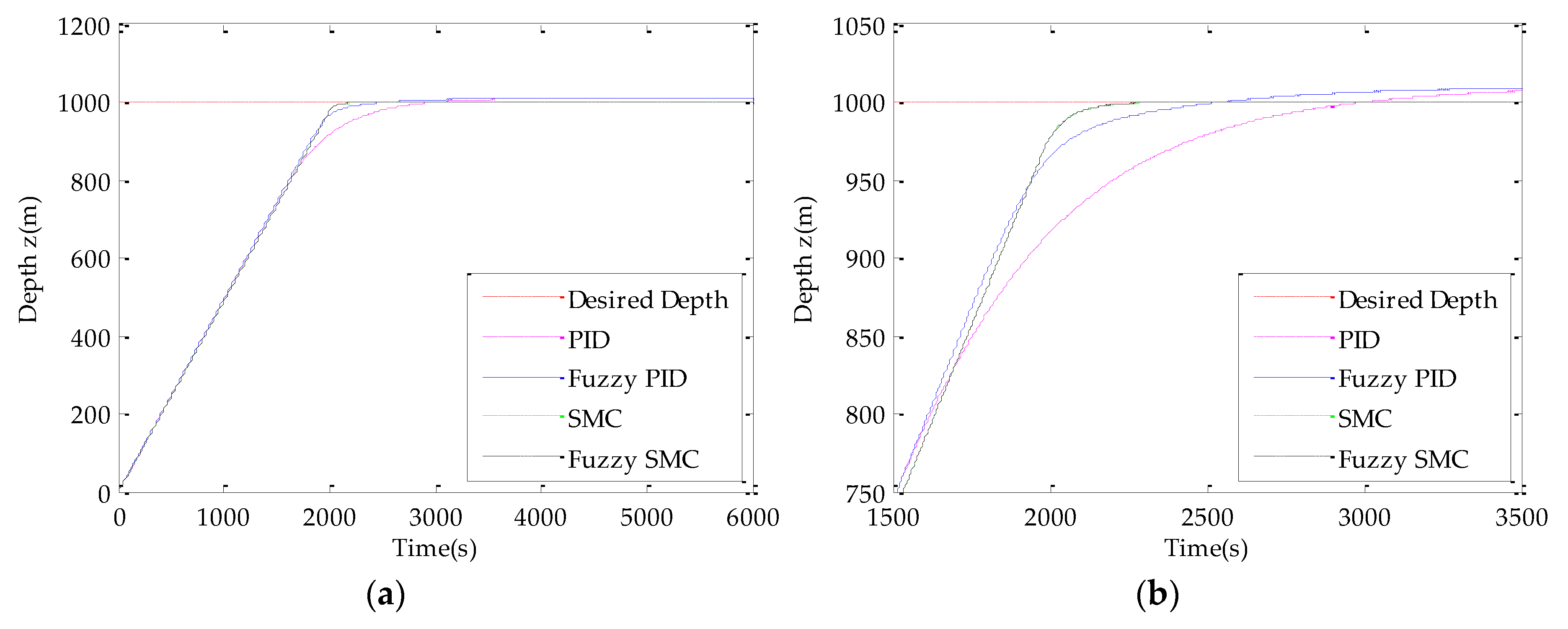
The depth control response curves of FOS with PID, fuzzy PID, sliding mode, and fuzzy sliding mode controllers are shown in Figure 11. It indicates that the depth response curves of the four control methods have almost no oscillation and tend to be stable. Approximately from 0–1500 s, the curves of the four controllers almost coincide due to the maximum volume flow rate of VBS. The velocity curves based on the four controllers are shown in Figure 12. It can be seen from the figure that the sinking speeds of the FOS with different controllers are 0.50 m/s (PID, Fuzzy PID), 0.49 m/s (SMC, Fuzzy SMC), respectively. For further analysis, characteristic response parameters obtained from the simulation results are presented in

Table 7. Characteristic parameter table of four controllers.

Controller Types	Rise Time (s)	Settling Time (s)	Steady-State Error (m)	Maximum Overshoot (%)
PID	1702.0	2671.5	10.2	1.027
F-PID	1610.6	2213.2	9.9	0.996
SMC	1632.7	2040.1	-0.2	≈ 0
F-SMC	1632.7	2040.0	-0.1	≈ 0

. Since the depth curves of SMC and fuzzy SMC methods do not reach 1000 with the steady-state error of -0.2 m, their maximum overshoots are approximately equal to 0.

Compared with the traditional PID controller, the fuzzy PID controller has better performance with the rise time reduced by 5.37%, the settling time decreased by 17.16%, the steady-state error decreased by 2.94%, and the maximum overshoot decreased by 3.02%. Compared with the sliding mode controller, the characteristic parameters of fuzzy sliding mode controller change a little. However, its velocity is more stable than the SMC method, which greatly saves its energy consumption. These indicate that in the depth control of FOS, the performance of fuzzy PID controller and fuzzy sliding mode controller is significantly better than pure PID controller and SMC controller. Furthermore, except for the rise time, the fuzzy sliding mode controller has shorter settling time (decreased by 7.8%), smaller steady-state error (decreased by 99.02%), and lower maximum overshoot compared with the fuzzy PID controller. The conclusion can be drawn that the designed fuzzy sliding mode controller has the advantages of fast response, high precision, and excellent steady-state performance without disturbing force.

4.2. Simulation and Analysis with Disturbing Force

To analyze the anti-interference ability of the designed controller, a disturbing force as Equation (24) is added to the system. The response curves of the four controllers in the presence of disturbing force are shown in Figure 13, of which the corresponding characteristic parameters are shown in

Table 8. Characteristic parameter table after adding interference to the four controllers.

Controller Types	Rise Time (s)	Settling Time (s)	Maximum Overshoot (%)
PID	1726.1	2693.9	1.057
F-PID	1615.3	2233.9	1.007
SMC	1633.3	2061.3	0.013
F-SMC	1632.6	2061.4	0.013

(due to the existing of the disturbing force, the response curves are fluctuating and the steady-state error does not exist.).

$$d=15\sin \left(\pi t/2\right)$$

(24)

In general, the parameters of these four control methods have changed while adding the disturbing force. To further compare the performance of the four control methods in the presence of disturbing force, the characteristic parameters without external disturbing force are subtracted from that with disturbing force, and the change of each parameter is shown in

Table 9. Changes of characteristic parameters.

Controller Types	Rise Time (s)	Settling Time (s)	Maximum Overshoot (%)
PID	+24.1	+22.4	+0.030
F-PID	+4.7	+20.7	+0.011
SMC	+0.6	+21.2	+0.013
F-SMC	-0.1	+21.4	+0.013

.

It shows that under the same conditions of disturbing force, the changes of parameters for fuzzy PID control, SMC, and fuzzy SMC are less than that for the PID control. While the changes of settling time have only slight differences among the four controllers, the change of rise time for the fuzzy SMC method is the littlest. Additionally, its maximum overshoot is always small. Therefore, the designed fuzzy SMC controller shows better anti-interference capability and robustness and has better dynamic performance.

5. Conclusions

For the depth control of FOS, its mathematical model has been obtained based on the hydrodynamic equation and on the characteristic parameters of the buoyancy control device with considering the variation of seawater density with depth. By simulating the processes of diving and suspending in the cases with and without disturbing force, the designed fuzzy sliding mode controller has been compared with a traditional PID controller, a fuzzy PID controller, and a sliding mode controller. The results demonstrate that in both cases, the fuzzy sliding mode controller could achieve the expected depth in the nearly shortest time with the minimum steady-state error and overshoot, which indicates its rapid response capability, good stability, and high accuracy. In addition, its change of rise time caused by disturbing force is smaller than the other three controllers. This indicates its possession of good robustness and anti-interference ability. Moreover, the consideration of the changes of seawater density with depth in the design of the depth controller for FOS to enable the adaptive adjustment in real time is a highlight for the controller design. Therefore, we carefully draw the conclusion that the proposed fuzzy sliding mode controller could satisfy the depth control requirements of FOS.

In the application of depth control for the similar underwater vehicle, if a PID controller must be used, the fuzzy logic method can be implemented with it as fuzzy PID to reach the stable depth faster. If a sliding mode controller is able to be used, it is better than PID and F-PID, but it cannot guarantee the stability of the actuator. If good depth response performances and actuator stability are required at the same time, the fuzzy sliding mode controller is much better. However, in our research, there remains some issues here that the anti-interference performance of the FOS is still not optimal, so an observer will be considered in our next step work, and the experiments in South Sea shall be carried out to test FOS performances.

References

1. Ding, W.; Huang, H.; Zhu, X.; Sun, G.; Niu, X. A new mobile oceanic seismic recording system and its application in marineseismic exploration. Prog. Geophys. 2019, 34, 292–296. [Google Scholar]
2. Hello, Y.; Ogé, A.; Sukhovich, A.; Nolet, G. Modern mermaids: New floats image the deep Earth. EOS Trans. Am. Geophys. Union 2011, 92, 337–338. [Google Scholar] [CrossRef]
3. Sukhovich, A.; Bonnieux, S.; Hello, Y.; Irisson, J.; Simons, F.J.; Nolet, G. Seismic monitoring in the oceans by autonomous floats. Nat. Commun. 2015, 6, 8027. [Google Scholar] [CrossRef] [PubMed] [Green Version]
4. Nolet, G.; Hello, Y.; van Der Lee, S.; Bonnieux, S.; Ruiz, M.C.; Pazmino, N.A.; Deschamps, A.; Regnier, M.M.; Font, Y.; Chen, Y.J. Imaging the Galápagos mantle plume with an unconventional application of floating seismometers. Sci. Rep. 2019, 9, 1326. [Google Scholar] [CrossRef] [PubMed] [Green Version]
5. Jones, N. Global seismic network takes to the seas. Nature 2014, 507, 151. [Google Scholar] [CrossRef] [PubMed] [Green Version]
6. Nolet, G. MERMAID seismometry in the oceans: Resolving the detail of geodynamic processes. In Proceedings of the EGU General Assembly Conference Abstracts, Vienna, Austria, 17–22 April 2016; Volume 18. [Google Scholar]
7. Simons, F.J.; Dando, B.D.E.; Allen, R.M. Automatic detection and rapid determination of earthquake magnitude by wavelet multiscale analysis of the primary arrival. Earth Planet. Sci. Lett. 2006, 250, 214–223. [Google Scholar] [CrossRef]
8. Joubert, C.; Nolet, G.; Bonnieux, S.; Deschamps, A.; Dessa, J.X.; Hello, Y. P-Delays from floating seismometers (MERMAID), part I: Data processing. Seismol. Res. Lett. 2016, 87, 73–80. [Google Scholar] [CrossRef]
9. Simons, F.J.; Nolet, G.; Georgief, P.; Babcock, J.M.; Regier, L.A.; Davis, R.E. On the potential of recording earthquakes for global seismic tomography by low-cost autonomous instruments in the oceans. J. Geophys. Res. Solid Earth 2009, 114, B5307. [Google Scholar] [CrossRef] [Green Version]
10. Zanoli, S.M.; Conte, G. Remotely operated vehicle depth control. Control Eng. Pract. 2003, 11, 453–459. [Google Scholar] [CrossRef]
11. Bessa, W.M.; Dutra, M.S.; Kreuzer, E. Depth control of remotely operated underwater vehicles using an adaptive fuzzy sliding mode controller. Robot. Auton. Syst. 2008, 56, 670–677. [Google Scholar] [CrossRef]
12. Wei, H.; Dong, Y. Adaptive Fuzzy Neural Network Control for a Constrained Robot Using Impedance Learning. IEEE Trans. Neural Netw. Learn. Syst. 2017, 29, 1174–1186. [Google Scholar]
13. Geng, T.; Zhao, J. Generalized predictive control with constraints for autonomous underwater vehicle depth control. In Proceedings of the 2012 International Conference on Modelling, Identification and Control, Wuhan, China, 24–26 June 2012; pp. 618–623. [Google Scholar]
14. Debitetto, P.A. Fuzzy logic for depth control of Unmanned Undersea Vehicles. IEEE J. Ocean. Eng. 1995, 20, 242–248. [Google Scholar] [CrossRef]
15. Li, H.; Wang, X.; Song, S.; Li, H. Vehicle control strategies analysis based on PID and fuzzy logic control. Procedia Eng. 2016, 137, 234–243. [Google Scholar] [CrossRef] [Green Version]
16. Khodayari, M.H.; Balochian, S. Modeling and control of autonomous underwater vehicle (AUV) in heading and depth attitude via self-adaptive fuzzy PID controller. J. Mar. Sci. Tech. 2015, 20, 559–578. [Google Scholar] [CrossRef]
17. Esfahani, H.N.; Azimirad, V.; Danesh, M. A Time Delay Controller Included Terminal Sliding Mode and Fuzzy Gain Tuning for Underwater Vehicle-Manipulator Systems. Ocean Eng. 2015, 107, 97–107. [Google Scholar] [CrossRef]
18. Skjong, S.; Pedersen, E. Model-based control designs for offshore hydraulic winch systems. Ocean Eng. 2016, 121, 224–238. [Google Scholar] [CrossRef]
19. Hu, J.; Hu, D.; Xiao, J. Research on motion control and simulation of underwater vehicle based on fuzzy theory. Sh. Sci. Technol. 2017, 39, 59–63. [Google Scholar]
20. Mehndiratta, M.; Kayacan, E.; Kumbasar, T. Design and experimental validation of single input type-2 fuzzy PID controllers as applied to 3 DOF helicopter testbed. In Proceedings of the 2016 IEEE International Conference on Fuzzy Systems (FUZZ-IEEE), Vancouver, BC, Canada, 24–29 July 2016; pp. 1584–1591. [Google Scholar]
21. Zhang, W.; Wang, H.; Bian, X.; Yan, Z.; Xia, G. The application of self-tuning fuzzy PID control method to recovering AUV. In Proceedings of the IEEE Oceans, Hampton Roads, VA, USA, 14–19 October 2012; pp. 1–5. [Google Scholar]
22. Fang, Y.; Fei, J.; Hu, T. Adaptive backstepping fuzzy sliding mode vibration control of flexible structure. J. Low Freq. Noise Vib. Act. Control 2018, 37, 1079–1096. [Google Scholar] [CrossRef] [Green Version]
23. Wang, Y.; Karimi, H.R.; Shen, H.; Fang, Z.; Liu, M. Fuzzy-model-based sliding mode control of nonlinear descriptor systems. IEEE Trans. Cybern. 2018, 49, 3409–3419. [Google Scholar] [CrossRef] [Green Version]
24. Li, J.P. Research on Buoyancy Regulating System and Depth Control Technology of Underwater Vehicle. Master’s Thesis, Harbin Engineering University, Harbin, China, 2010. [Google Scholar]
25. Roberts, G.N.; Sutton, R. Advances in Unmanned Marine Vehicles; Institution of Electrical Engineers: London, UK, 2006; Volume 69. [Google Scholar]
26. Zhang, C.; Shen, Y.; Wu, Y.; Wu, G.; Liu, X.; Huang, H. Depth Control of Floating Ocean Seismograph Based on Variable Buoyancy System. In Proceedings of the OCEANS 2018 MTS/IEEE Charleston, Charleston, SC, USA, 22–25 October 2018; pp. 1–4. [Google Scholar]
27. Sun, Y.Q.; Ma, Y.Y.; Deng, Z.C. Modern Maneuver Theory and Application of Submarine and Deep-Diving Submersible Vehicle; National Defense Industry Press: Beijing, China, 2011. [Google Scholar]
28. Wang, T.; Ye, X.; Wang, L.; Li, H. Grid Search Optimized SVM Method for Dish-like Underwater Robot Attitude Prediction. In Proceedings of the Fifth International Joint Conference on Computational Sciences and Optimization, Harbin, China, 23–26 June 2012; pp. 839–843. [Google Scholar]
29. Huang, K.L.; Pang, Y.J.; Yu-Ming, S.U.; Zhu, J. Research on linearity hydrodynamic coefficients calculation method of submergible vehicle. J. Sh. Mech. 2008, 12, 697–703. [Google Scholar]
30. Chen, J.; Xing, J. Depth control of submarine based on fuzzy adaptive PID. Sh. Sci. Technol. 2011, 33, 56–60. [Google Scholar]
31. Yang, S.; Li, K.; Jiao, S. Design and Simulation of the Longitudinal Autopilot of UAV Based on Self-Adaptive Fuzzy PID Control. In Proceedings of the International Conference on Computational Intelligence and Security, Beijing, China, 11–14 December 2009; pp. 634–638. [Google Scholar]
32. Li, J. Research on Motion Control of a Manned Underwater Vehicle Model Based on Fuzzy PID Control. Master’s Thesis, Harbin Engineering University, Harbin, China, 2012. [Google Scholar]
33. Wang, Y.; Zheng, R.; Wu, J. Research on AUV Depth Control Based on the Variable Buoyancy System. Autom. Instrum. 2015, 4, 6–10. [Google Scholar]
34. Hammad, M.M.; Elshenawy, A.K.; El Singaby, M.I. Trajectory following and stabilization control of fully actuated AUV using inverse kinematics and self-tuning fuzzy PID. PLoS ONE 2017, 12, e179611. [Google Scholar] [CrossRef] [PubMed] [Green Version]
Figure 1. Working principle diagram of the floating ocean seismograph (FOS).
Jmse 08 00166 g001
Figure 2. Outside view of floating ocean seismograph.
Jmse 08 00166 g002
Figure 3. Vertical plane motion coordinate system.
Jmse 08 00166 g003
Figure 4. Seawater density fitting curves vary with depth at a point of South China Sea.
Jmse 08 00166 g004
Figure 5. Depth control block diagram.
Jmse 08 00166 g005
Figure 6. Proportional–integral–derivative (PID) depth controller block diagram.
Jmse 08 00166 g006
Figure 7. Fuzzy PID depth controller block diagram (ke and kee are adjustment for fuzzy inference inputs; α, β, and γ are correction factors for fuzzy inference outputs).
Jmse 08 00166 g007
Figure 8. Block diagram of fuzzy sliding mode depth controller.
Jmse 08 00166 g008
Figure 9. Types of membership function of input and output variables.
Jmse 08 00166 g009
Figure 10. Depth response of PID depth controller.
Jmse 08 00166 g010
Figure 11. Control response curves without disturbing force. (a) Depth response curves. (b) Magnified view of depth response curves.
Jmse 08 00166 g011
Figure 12. Velocity curves of depth control without disturbing force.
Jmse 08 00166 g012
Figure 13. Control response curves with disturbing force. (a) Depth response curves. (b) Magnified view of depth response curves.
Jmse 08 00166 g013