Wake behind a Compound Wing in Ground Effect

Abstract

Flow structure is a crucial point for the conceptual design of Wing-in-Ground effect (WIG) crafts. In this study, pressure distributions around a compound wing, velocity and the turbulent intensity distribution in the wake area after trailing of the wing, have been investigated numerically. Computational simulations were completed regarding various angles of attack in-ground-effect. Two parts made up the compound wing: The first composed by one rectangular wing in the center, the second composed by a reverse taper wing, consisting of an anhedral angle at the side. A realizable k-ε turbulent model exhibited the flow field in the physical domain about the wing surface. The numerical results of the compound wing were validated using the data provided by wind tunnel tests. The flow structures around the compound wing were compared with that of a rectangular wing for different conditions. It was found that the pressure distribution on the rectangular wing was weaker than at the lower surface for the compound wing. However, the suction effect on the upper surface of the rectangular wing was higher. Also, the velocity defect and the turbulence level in the wake area was greater behind the compound wing.

1. Introduction

The Wing-In-Ground (WIG) effect vehicles are unconventional vehicles that are designed to attain sustained flight over a level surface (usually over the sea), by making use of the ground effect. This unconventional vehicle could be an interesting transportation solution due to some specific aspects. The WIG effect vehicles are a very-fast transportation system, and do not require any large infrastructure (e.g airports, runways, etc.). In fact, the WIG effect vehicles are a transportation way extremely fast like an airplane, but are able to dock/undock like a small boat as well. However, differently from a boat, they have a power-to-weight ratio higher than a fast boat (typically a planing hull). Furthermore, they are able with the same installed power to reach a speed at least twice that of a planing hull with comparable installed power.

For these reasons, this kind of transportation system could represent an effective solution, in particular in the archipelagic areas (e.g., South-East Asia, Oceania Islands, the Aegean Islands, etc.).

The development of WIG craft was initiated in the early 1960s, when the first researchers and developers tried to exploit the favorable aerodynamic behavior of wings near a ground surface (e.g., water, ice and snow). The researchers have attempted to create advantages for the ground effect for many civilian and military applications by means of WIG effect vehicles. The increase of lift and drag-reduction for the WIG are the main benefits when WIG crafts fly close to the ground. At low ground clearance, the immobility point transfers to the lesser exterior of the wing, and consequently, an air cushion is generated, which leads to the existence of the highest pressure, i.e., the ram pressure. In addition, the drag force drops because the downwash velocity decreases when the wing reaches the ground, as indicated in Ahmed and Sharma [1].

The ground level represents a constraint for the structure of flow below the suction exterior of the overturned wing. The flow accelerates significantly, while the wing moves toward the proximity of the ground. Thus, resulting in a greater suction force, and accordingly, more force downwards in comparison with a freestream condition, as shown in Zerihan and Zhang [2].

Many researchers have demonstrated the same downforce behavior of an inverted wing, although the reasons are different for the downforce-reduction phenomenon. Ranzenbach and Barlow [3] believed that the merging of boundary layers with the ground is the main reason for the reduction of downforce at low critical height. However, Zerihan and Zhang [2] demonstrated that this phenomenon is related to the increase in adverse pressure gradients. For this reason, boundary layer separation is developed on the suction surface with the reduction of ground level. Pailhas et al. [4], Vassiloulos and Gai [5] and Khorrami et al. [6] investigated the wake and vortex shedding on an airfoil with a finite trailing edge. Pailhas et al. [4] investigated the dense trailing edge of a wing with Laser Doppler Anemometry (LDA). These researchers observed two counter-rotating vortices in the trailing edge, and explored the downstream flow.

Zhang and Zerihan [7] analyzed the turbulent wake flow in the back of the trailing edge of an overturned airfoil in the ground closeness by means of experimentation. They showed a decrease in the height of a wing when the wake region grew. They could not measure the exact thickness of the wake area, due to the merging of the wake with the ground. The top of the wake region was recorded as constant, while the bottom of the wake dropped when the height of the airfoil decreased. The extension of the wake area toward the ground was related to the rise of the maximum velocity deficit as the ground clearance reduced. The rise of an adverse pressure gradient led to the separation of the boundary layer on the suction surface in a small ground level, and consequently, the wake area would be wide.

Galoul and Barber [8] carried out a flow visualization for an inverted wing, with endplates using smoke trace and LDA. The authors examined the effects of height and endplates on the velocity field and turbulence intensity behind the wing. A small width endplate was used in the simulations. The presence of these endplates enhanced the downforce as the tip vortex was lessened. In addition, the flow behavior on the wing would be similar for two-dimensional flow. Conversely, the different pressure on the upper surface and bottom surface generated two co-rotating vortices at the up and down of the endplate. The flow behavior in both vortices was affected by the size of endplates. According to their visualizations, the longitudinal velocity in the vortices was lower than in freestream. This deficit was produced with the high rotational velocity that caused low pressure at the core of the vortices. Hence, the vortex would be strong when the longitudinal velocity was low at its core. The ground clearance of airfoils influences the wake region behind the trailing edge significantly; see Wen et al. [9].

Further, Hsiun and Chen [10] showed that the principal aerodynamic coefficients of two-dimensional airfoils could be affected via the form of the area across the lower side of the airfoil and the free surface of the ground. Wen et al. [9] studied the wake flow behavior at the trailing edge of the airfoil with respect to the different airfoil height from the free surface. The airfoil was mounted at the upper boundary layer of the free surface. Later, the authors concentrated upon analyzing the influence of free surface on the wake flow structures.

According to the investigational outcomes, they found that the vortex shedding from the lower side of the airfoil was evidently affected by the free surface. When the height of the airfoil decreased, the expansion of reverse flow in the back of the trailing edge of an airfoil was observed because of the shift of the separation point to the leading edge.

Zhang and Zerihan [11] investigated the wake region located in the downstream of an overturned wing by means of experimentation. It was displayed that when the motion was downstream, there was an increase in the wake size. However, there was a decrease in the velocity deficit. At the time the wing advanced to the ground, the denser wake and greater velocity deficit were observed. The oppositional flow of the pressure gradient was detected across the wake region and the ground exterior.

Zerihan and Zhang [12] investigated the aerodynamics of a wing with a Gurney flap. According to the flow separation on the wing with a Gurney flap, the reduction of downforce was sharper than the clean wing. Gurney flaps produced a larger and thicker wake compared with the clean wing. In addition, the authors observed a thick wake as the ground clearance decreased.

The momentum of the flow was diminished by a high adverse pressure gradient; then, the flow separation appeared from the wing surface [13,14]. Various processes are available for flow dissociation control; for example, vortex generator jets and vortex generators (VGs) [15,16]. These devices improve the momentum of the boundary layer by transferring the momentum from the outer flow to the boundary layer flow.

Zerihan and Zhang [17] investigated the pressure scattering and wake area throughout a single element in a numerical manner. A Reynolds-Averaged Navier–Stokes (RANS) approach was applied for two-dimensional imagery with a designed grid, and the k-ω SST and Spalart–Allmaras turbulence replicas were engaged for the unstable flow definition throughout the wing. Mahon and Zhang [18] demonstrated that k-ω SST and realizable k-ε turbulence models are suitable for estimating the pressure distributions and the visualization of wake region, respectively. They used multiblock hybrid grids. Also, Kieffer et al. [19] applied the standard k-ε turbulence model for a racing car wing.

Soso and Wilson [20] performed an experimental analysis in order to research the aerodynamic performance of an inverted wing-in-ground effect in the wake region. A diffuser bluff body with a back wing created this wake area. A higher downforce reduction was observed as the wing’s ground clearance went up. Then the authors discovered that almost all of the portions of this decrease were associated with the wing suction exterior. Furthermore, Soso and Wilson [21] examined the consequences of the height of the bluff body and the diffuser ramp angle on the downstream wing-in-ground effect in a wind tunnel. The authors demonstrated that the stiffness of the downstream wing’s wake area expanded with the decrease of the bluff body height.

Ahmed and Sharma [1] experimentally investigated the velocity distribution on the wake region and the pressure distribution on a symmetrical wing. They showed that the pressure coefficient on the suction surface had an insignificant effect alongside ground clearance, particularly for greater attack angles. Therefore, the improvement of the lift force is due to the enhancement of the distribution of pressure on the surface of pressure. Additionally, the authors recorded an extremely thick turbulent wake region for a high attack angle.

The reduction of suction force on the upper surface of a multi-element airfoil was higher than the increment of pressure at the lower surface with reduction of the ground clearance, and according to the pressure distribution for a multi-element airfoil, the lift force diminished. In addition, the vortices became stronger, and were recorded when the height decreased, as reported in Xuguo et al. [22].

As previously noted, the investigation of the flow structure around a wing close to the ground is a critical task. Several researchers identified that the flow field around a wing still exhibits a lack of information, especially around a special wing configuration. In this current research, the flow near a compound wing was inspected, similarly to Jamei et al. [23].

The special wing configuration, analyzed in the present research, is the compound wing which consists of three parts: Two reversal taper wings, with a dihedral angle at the sides, and a rectangular wing in the center (the aerodynamic characteristics and static stability for this type of wing have been evaluated in Jamei et al. [24,25], and the whole WIG craft has been examined in Mobassher et al. [26]). In this study, the distribution of pressure near the compound wing, velocity and turbulent intensity distributions in the wake region in the back of the wing was explored. In addition, the compound wing’s flow structure was compared with a rectangular wing. Furthermore, the velocity and turbulence contours related to both wings were presented for a better understanding. This research was carried out with respect to the various angles of attack in-ground-effect. Hence, this research demonstrated a comprehensive understanding of the physics of flow near the compound wing, and researchers and designers can ultimately utilize the information as an instruction for the WIG craft vehicles developing.

In this paper, the Computational Fluid Dynamics (CFD) numerical equations are presented in Section 2. Section 3 and Section 4 contain the grid independence analysis and numerical details. In Section 5 the validation process has been exposed. The main results of the paper are presented in Section 6. In Section 7 there are the conclusions, and finally in Section 8, an overview of the future works.

2. CFD Numerical Study

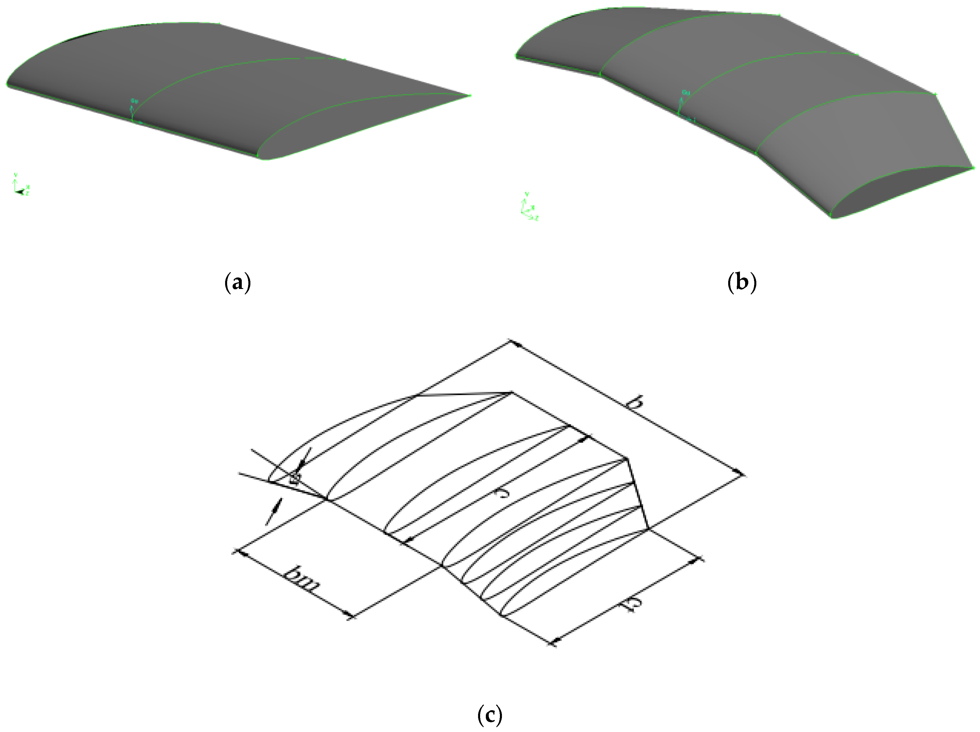
A computational investigation was performed using a compound wing (Jamei et al. [23]) and a common rectangular wing based on NACA 6409 airfoil section. The compound wing, as previously indicated, is a wing composed of three parts, one rectangular wing in the middle, and two reverse taper wings with an anhedral angle on the sides (Figure 1b,c).

Table 1. Principle dimensions of the compound and rectangular wings.

Dimension	Rectangular Wing	Compound Wing
Total wing span (b)	250 mm	250 mm
Root chord length (c)	200 mm	200 mm
Middle wing span (bm)	-	125 mm
Taper ratio (c/ct)	-	1.25
Anhedral angle (a) [°]	-	13°

and Figure 1 displays the key compound wing’s dimensions and the rectangular wing. This simulation campaign was developed with different attack angles and ground clearance (h/c) of 0.15, consisting of an aspect ratio of 1.25. The velocity of air in the free stream was 25.5 m/s. Meanwhile, the ground was considered as moving to remove the ground boundary layers. Ground level (h) is expressed as the distance between the trailing edge of the wings’ center and the ground surface.

The simulations were performed using the commercial code ANSYS-FLUENT. The governing equation, which is used in the CFD simulations is RANS, as the following:

$$\frac{\partial }{\partial t}(\rho {\overline{u}}_i)+\frac{\partial }{\partial x_j}(\rho {\overline{u_{j}u}}_i)+\frac{\partial }{\partial x_j}(\rho \overline{u_j^{’}{u}_i^{’}})=-\frac{\partial \overline{p}}{\partial x_i}+(\mu +{\mu }_t)\frac{{\partial }^2{\overline{u}}_i}{\partial x_j\partial x_i},$$

(1)

where, ρ, $\overline{u}$, $\overline{p}$, u’, µ, and µt are the density of the fluid, time-mean velocity, time-mean pressure, fluctuating velocity, total viscosity and turbulent viscosity, respectively. As a result of RANS, Reynolds stresses appear in the equation that needs to be modeled. So, turbulent modeling has been considered for this issue.

The turbulent flow around the wings was proposed as incompressible and steady-state, using a realizable k-ε turbulence model. The k-ε is based on determining µ_t by solving two transport equations, one for the turbulent kinetic energy (k) and the other for the rate of dissipation of turbulent kinetic energy (ε). Turbulent viscosity has been determined by Equation (2).

$${\mu }_t=\rho C_{\mu }\frac{k^2}{\epsilon },$$

(2)

where, $C_{\mu }$ is a constant value. The turbulent dissipation energy (ε) and the turbulent kinetic energy (k) have been calculated as follows:

$$\frac{\partial }{\partial t}(\rho k)+\frac{\partial }{\partial x_j}(\rho k{u}_j)=\frac{\partial }{\partial x_j}\left[\left(\mu +\frac{{\mu }_t}{{\sigma }_k}\right)\frac{\partial k}{\partial x_j}\right]+G_k+G_b-\rho \epsilon -Y_M+S_k,$$

(3)

$$\frac{\partial }{\partial t}(\rho \epsilon )+\frac{\partial }{\partial x_j}(\rho \epsilon u_j)=\frac{\partial }{\partial x_j}\left[\left(\mu +\frac{{\mu }_t}{{\sigma }_{\epsilon }}\right)\frac{\partial \epsilon }{\partial x_j}\right]+\rho C_{1}S\epsilon -\rho C_2\frac{{\epsilon }^2}{k+\sqrt{\nu \epsilon }}+C_{1\epsilon }\frac{\epsilon }{k}{C}_{3\epsilon }{G}_b+S_{\epsilon }.$$

(4)

where C_k represents the generation of turbulence kinetic energy due to mean velocity gradients, G_b is the generation of turbulence kinetic energy due to buoyancy, Y_M represents the contribution of the fluctuation dilation in the compressible turbulence to the overall dissipation rate, S_ε and S_k are the user-defined source terms respectively, σ_ε and σ_k are the Prandtl numbers for k and ε, respectively, C_1ε, C₂ and C_3ε are the adjustable constants, and S is the wing planform area (C_1ε = 1.44, C₂ = 1.9, σ_k = 1.0, and σ_ε = 1.2). S and C₁ have been defined as follows:

$$S=\sqrt{2S_{ij}{S}_{ij}},$$

(5)

$$C_1=\max \left[0.43,\frac{k}{k+5\epsilon }\right],$$

(6)

where S_ij is the mean rate of the tensor of deformation.

The aerodynamic coefficients and center of pressure in this numerical study were determined as follows:

$$C_L=\frac{L}{0.5\rho U^{2}A},$$

(7)

$$C_D=\frac{D}{0.5\rho U^{2}A},$$

(8)

$$C_M=\frac{M}{0.5\rho U^{2}Ac},$$

(9)

where L is lift force, D is the drag force, M is the moment, A is the area of the wing. So, the center of the pressure can be calculated according to Equation (10).

$$X_{CP}=0.25+\frac{C_M}{C_L\cos \alpha +C_D\sin \alpha }.$$

(10)

where α is the angle of attack, C_L, C_D, and C_M are the lift coefficient, drag coefficient and the moment coefficient, respectively.

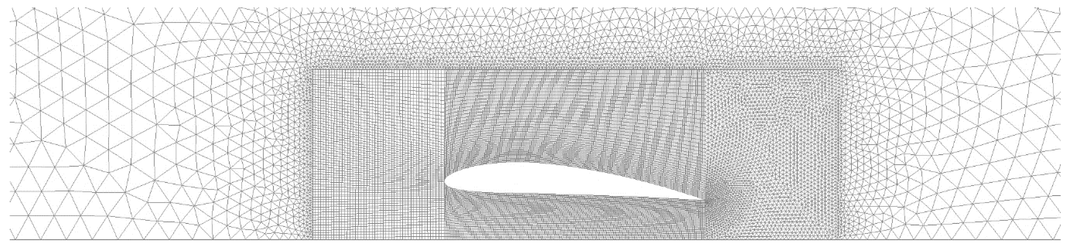
In these simulations, the cells number was about 4,500,000. This number of mesh elements was chosen in order to support high resolution for flow characteristics around the wings. A coupled way of structured (near the wing) and unstructured (far-field) mesh has been applied, as shown in Figure 2.

3. Numerical Setup

The second-order upwind scheme was applied for the discretization of turbulent kinetic energy, momentum equations and turbulent dissipation energy. In addition, the Reynolds stress problem is solved by means of the k-ε turbulence model. The Semi-Implicit Method for Pressure-Linked Equations (SIMPLE) technique was utilized, so that velocity and pressure are coupled.

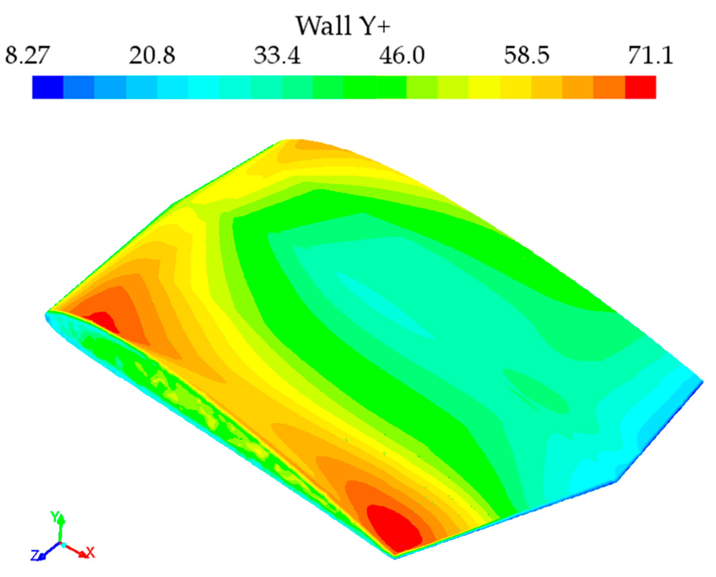
In order to improve the accuracy of this numerical simulation, the turbulent boundary layer must be checked in where the viscosity-affected regions have large gradients in the solution variables. An accurate representation of the near-wall region is determined by the y⁺. The y⁺ is a non-dimensional wall distance for a wall-bounded flow, and it can be defined in the following way:

$$y^{+}=\frac{u^{*}y}{\nu },$$

(11)

where u* is the friction velocity at the nearest hull, y is the distance to the nearest wall, and ν is the local kinematic viscosity of the fluid.

The y⁺ value on the wing surface in turbulent flow was recorded between 10 and 120 (see Figure 3); moreover, it had an acceptable accuracy in the present simulation if a standardized wall function was applied.

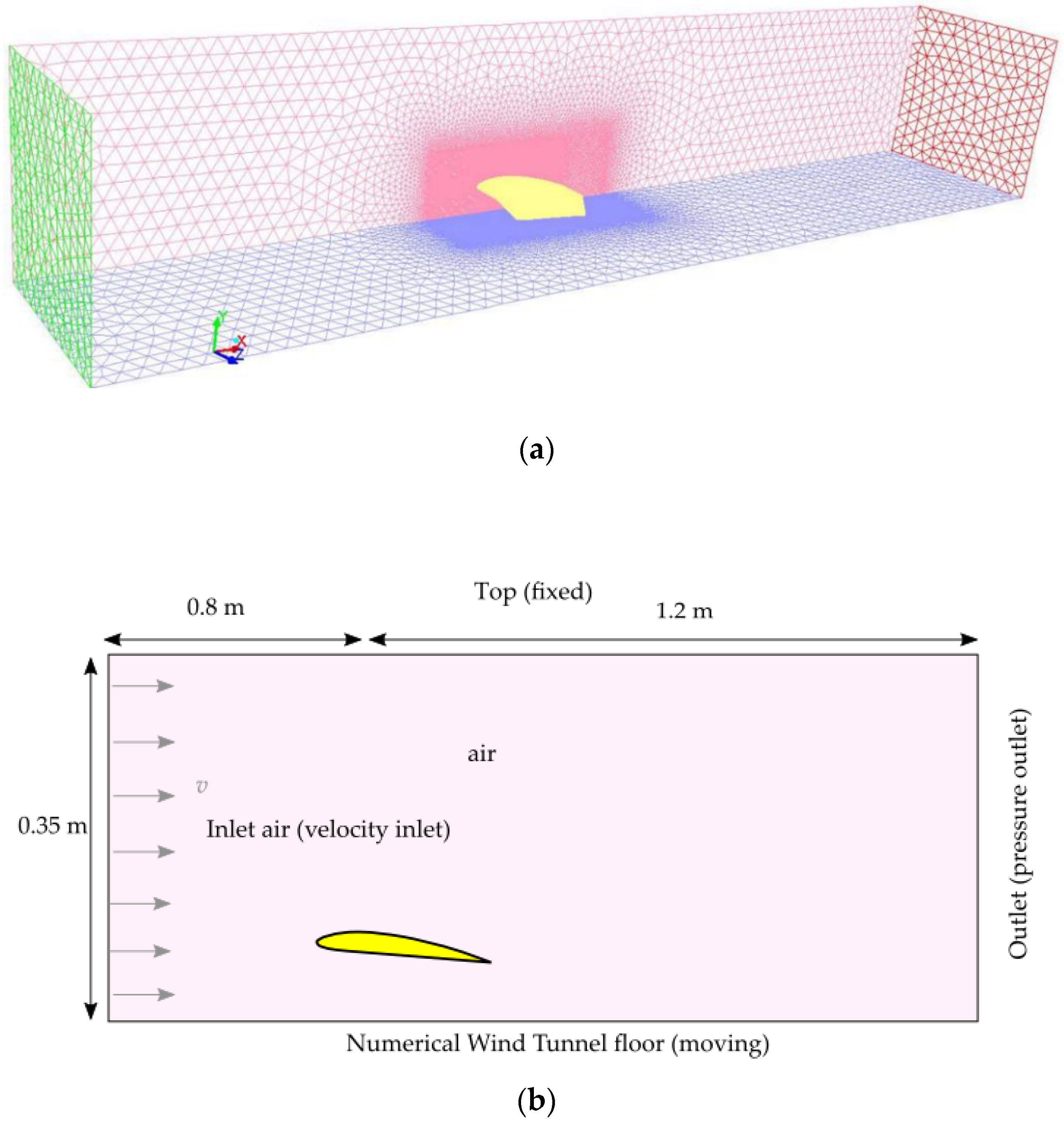
A symmetry-plane was utilized for the compound wing, as shown in Figure 4a, in order to reduce the computational effort.

These simulations were accomplished by the proper physical computational domain, which confirmed that no blockage consequences from the top and the side boundaries were detected. The main dimensions are exposed in Figure 4b. Furthermore, enough space was present across the surface of the wings and the inlet and outlet limitations to prevent connections within them.

As stated before, the simulation campaign was carried out considering the ground (Numerical Wind Tunnel floor) as moving, as indicated in Figure 4b. However, only the validation simulations have been performed with the fixed ground, in order to follow the experimental conditions. No-slip solid and smooth walls were used for the definition of these wings’ surface, ground boundary and the sides of the physical domain. Uniform inlet velocity and outlet pressure without a pressure gradient were engaged on the upstream and downstream, respectively.

4. Mesh Convergence and Verification Analysis

The verification process is the assessment of the simulation uncertainty (U_SN), as indicated in Stern et al. [27]. The grid uncertainty, generally, represents the main sources of numerical uncertainty (e.g., Wilson et al. [28]).

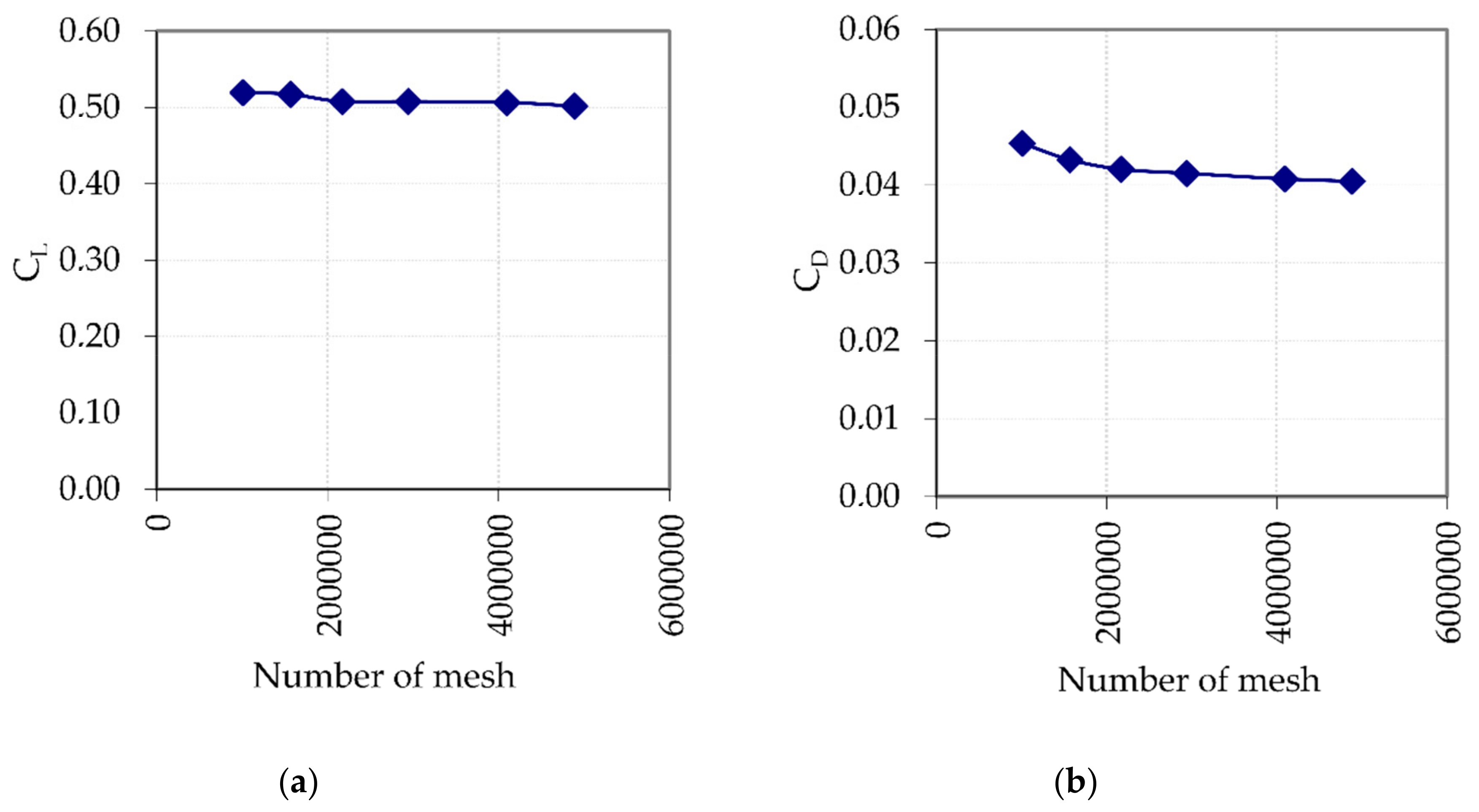
In order to evaluate the mesh effect on the results, a preliminary mesh convergence estimation of the numerical simulation results has been carried out (Figure 5). According to Figure 2, the lift coefficient and drag coefficient values show a convergent trend for the high numbers of cells.

As the second stage, the grid uncertainty (U_G) was evaluated using the Grid Convergence Index (GCI) method (Roache [29,30]), considering the modified version proposed by Eça and Hoekstra [31,32]. This modified approach is based on the Least-Squares Root (LSR) applied to the GCI method. The LSR method is used to minimize the square root of the squares of the residuals in Equation (12):

$$f\left(S_0,q,p_k\right)=\sqrt{{\displaystyle \sum _i^{n_g}{\left(S_i-\left(S_0+q_i{r_k}^{p_k}\right)\right)}^2}},$$

(12)

where n_g is the number of the grid tested, q_i is the coefficient of the i^th order error term, S₀ is the exact solution, p_k is the observed order of accuracy, and r_k defines a constant refinement ratio. The minimum of function f is found by setting its derivatives with respect to S₀, q and p_k equal to zero. Evaluating S₀, q and p_k, it is possible to calculate the error due to the mesh applying the generalized Richardson extrapolation method. More details about this method are available in Eça and Hoekstra [31,32].

The evaluated grid uncertainty for C_L is equal to 4.43% of the finest grid result, and for C_D is equal to 15.01% of the finest grid result. For the L/D, the grid uncertainty is equal to 19.44% of the finest grid result. Other sources of uncertainty, as the iterative uncertainty (U_I), are found to be negligible with respect to grid uncertainty, similarly to what happens in other cases (e.g., Wilson et al. [28], Xing et al. [33], and De Marco et al. [34]).

The simulation Uncertainty (U_SN), according to Stern et al. [27], is defined as follows:

$$U_{SN}^2=U_I^2+U_G^2+U_T^2+U_P^2=U_I^2+{\displaystyle \sum _{j=1}^J{U}_j^2}$$

(13)

The U_P represents the other sources of uncertainty. For the abovementioned reasons the Equation (13) could be simplified as follows:

$$U_{SN}^2\approx U_G^2$$

(14)

Hence, the simulation uncertainty is for C_L equal to 4.43%, for C_D it is equal to 15.01%, and for the L/D, it is equal to 19.44%.

5. Validation of Numerical Study

The CFD simulation performed was compared against experimental results obtained with the use of the low-speed wind tunnel at the Universiti Teknologi Malaysia. This wind tunnel was not equipped by moving ground. The boundary layer thickness is about 40 mm in the wind tunnel’s test chamber. Additionally, the wind tunnel is able to provide air-flow speed up to 80.0 m/s in the test chamber. The test chamber dimensions are the following: 2.0 m of width, 1.5 m of height and 5.5 m of length. Some of the important features regarding the wind tunnel’s internal airflow are:

• the turbulence is < 0.06%,
• flow angularity uniformity < 0.15,
• temperature uniformity < 0.2,
• flow uniformity < 0.15%.

Furthermore, the wind tunnel consists of facilities with high-quality instrumentations that permit the repeatability and correctness of the experimental outcomes [25,35]. The experimental data uncertainty (U_D) of the wind tunnel tests were evaluated according to the ISO GUM procedures [36].

Hence, in order to validate the numerical results (S), the validation uncertainty U_V has been assessed using the experimental data uncertainty, according to the following formula [27,37].

$$U_V^2=U_D^2+U_{SN}^2$$

(15)

The comparison error was estimated using experimental data (D) and S as in the following equation.

$$E=D-S$$

(16)

To determine whatever value has been validated, E is compared with U_V. So, when:

• |E|  <  U_V, the combination of all of the errors in D and S is smaller than U_V, and validation is achieved at the U_V interval.
• |E|  >  U_V, the combination of all errors in both the simulation and in the experimental data is greater than the validation uncertainty. Then validation has not been achieved for this validation uncertainty level.
• U_V  <<  |E|, this case highlights the need to improve the simulation modeling.

The U_V and E results are available in

Table 2. Validation Uncertainty and Comparison Error for Drag coefficient and Lift-to-drag ratio for the compound wing at a velocity of 25.5 m/s and ground clearance of 0.15.

Angle of Attack	UV		│E│
(deg)	CD	L/D	CD	L/D
0	15.02%	19.47%	5.35%	6.59%
2	15.48%	20.07%	6.78%	15.86%
4	15.03%	19.48%	19.88%	20.08%
6	15.29%	19.81%	31.78%	12.82%
8	15.04%	19.55%	35.99%	7.75%

and Figure 6.

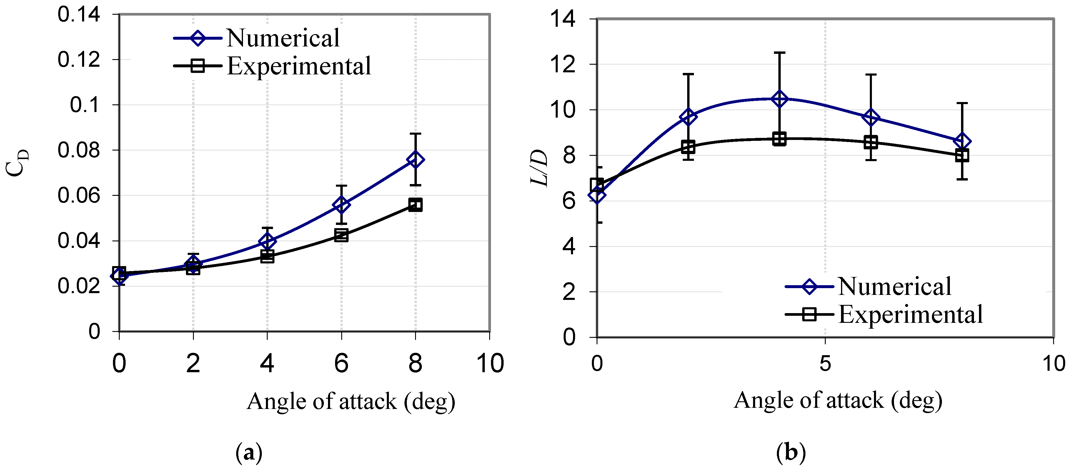
The drag and lift-to-drag ratio against the angle of attack of the compound wing simulated with fixed ground conditions and in a ground clearance of 0.15 is shown in Figure 6. The averages of errors for the drag coefficient and lift-to-drag ratio are 20.0% and 12.6%, respectively, as indicated in Jamei et al. [38].

The comparison between E and U_V shows that validation is achieved for the first two angles of attack for the C_D, and for L/D the validation is achieved for all the angles of attack except for the 4 deg. However, for the C_D, the validation process for the last two angles of attack highlights a shortcoming in the simulation modeling.

This issue was already clearly exposed in Jamei et al. [38], where the modelization error (e.g., turbulence models and wall functions) was found as one of the main sources of error besides the numerical error due to the mesh. The relevance of modelization error, as one of the two main sources of error and uncertainty in a simulation, is widely exposed in Stern et al. [27].

In this study, this modelization error could be related in particular to the simulation of a complex area, such as the ground boundary layer, characterized by a high gradient of pressure and velocity, in particular for the highest angles of attack. This modelization error was detected, in particular for the C_D, also in similar papers (e.g., De Marco et al. [34]). However, the overcoming of the modelization error could require a change from the RANS to an enhanced approach, such as the Large Eddy Simulation (LES).

6. Results and Discussions

As mentioned before, the present research investigated the flow around and behind a rectangular wing and a compound wing. For these purposes, the distribution of pressure near the wings and the wake area in the back of the trailing edges were shown for low ground clearance of 0.15, and for two attack angles: 4° and 6°.

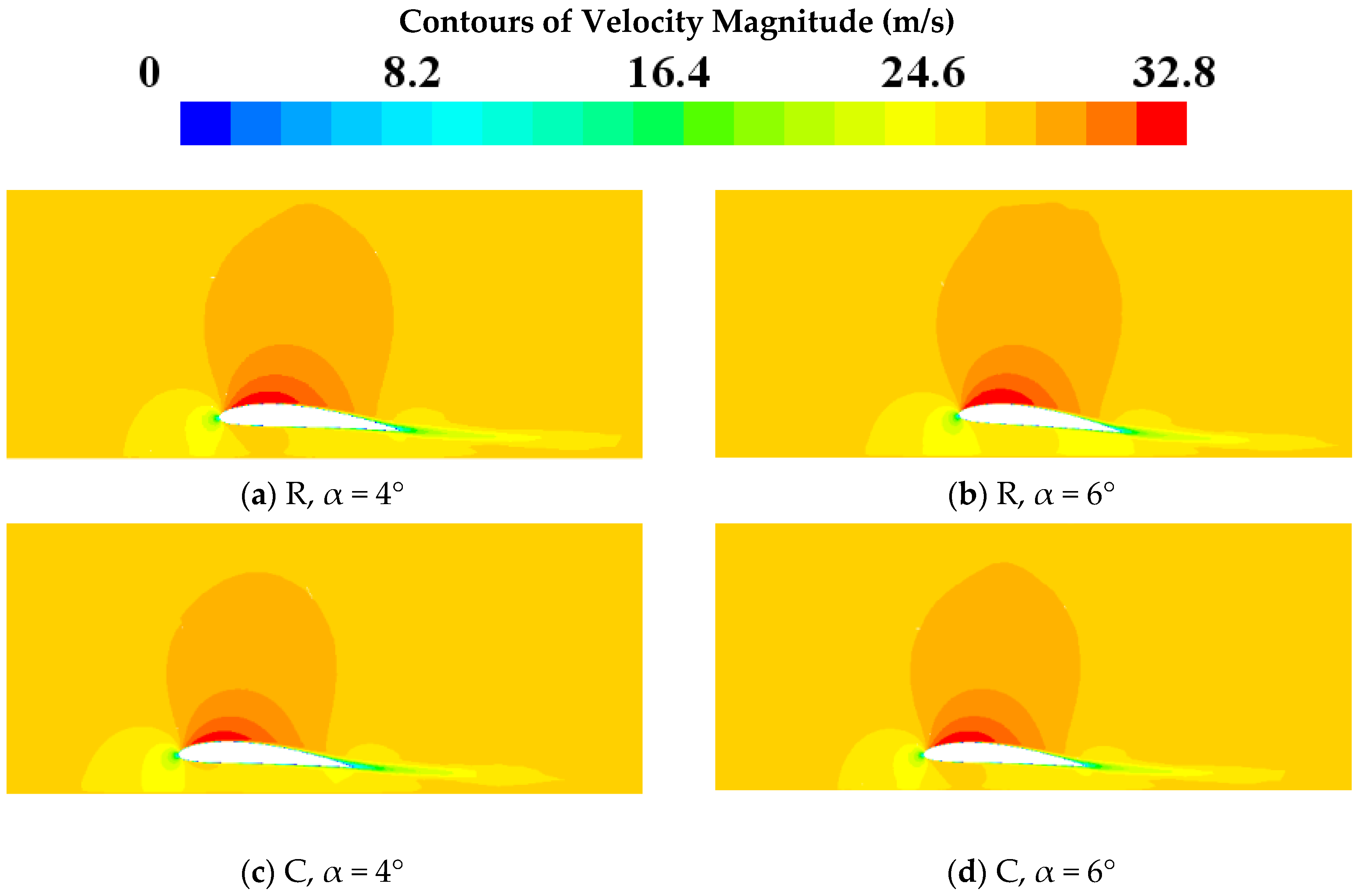
Figure 7 displays the velocity distribution around and behind the compound wing and the rectangular wing. Greater velocity scatterings were present in the middle span of both wings between the lower surface and moving ground at a lesser attack angle (α = 4°). Generally, the velocity under the compound wing surface was slighter than that of the rectangular wing, based on the Bernoulli equation, since the pressure must be greater for the compound wing. The movement of stagnating airflow from leading toward the lower surface was greater for the compound wing, which produced a higher ram effect. On the other hand, when the airflow was diverted to the upper surface with a lower momentum, then the suction effect was lower for the compound wing in comparison to that of the rectangular wing. According to the velocity distribution, the possibility for a separation of airflow for the compound wing was higher due to the lower energy of the airflow on the upper surface. The velocity distribution in the wake area behind the wings depicts that the velocity defect had an increment for both wings at a low ground clearance of 0.15 as the angle of attack increased. However, this defect was gradually higher for the compound wing.

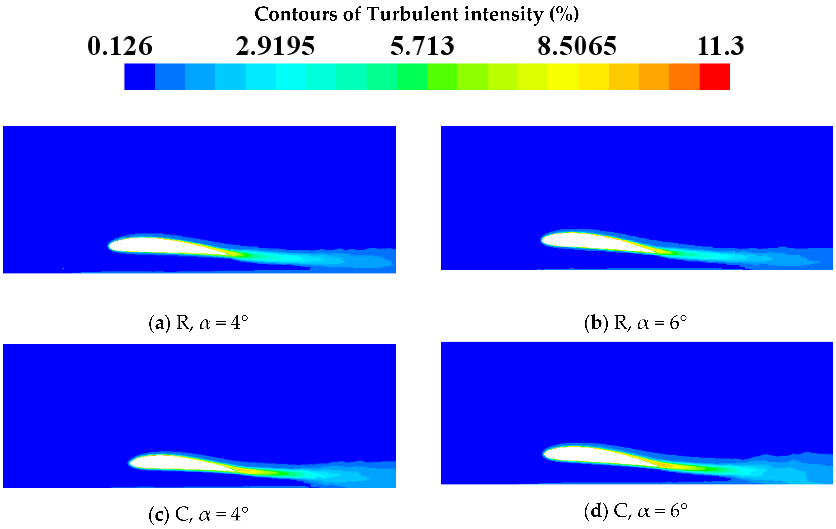
Figure 8 illustrates the turbulent intensity contours at the trailing edge and behind the wing-in-ground effect. When the angle of attack increased, the turbulence of airflow near the trailing edge of both wings was enhanced. The turbulent intensity in the proximity of the trailing edge of a compound wing was higher than in that of the rectangular wing, particularly at a higher angle of attack (α = 6°).

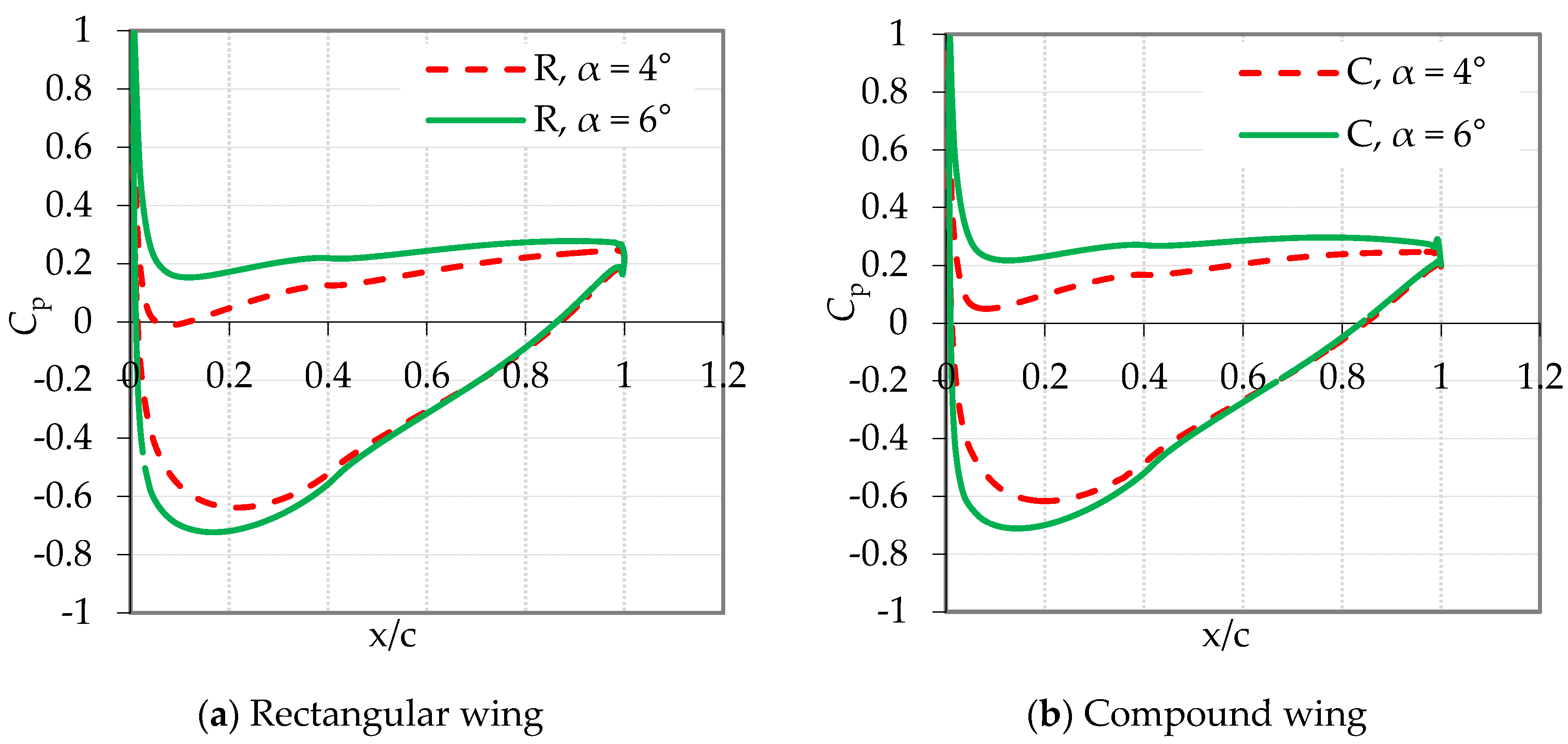
The variation of pressure coefficient (Cp) is shown in Figure 9 at the middle span of the surface of the compound wing and the rectangular wing at a low ground clearance of 0.15 for the various attack angles tested (4° and 6°). The positive pressure on the lower surface and negative pressure (suction effect) on the upper surface of both wings increased, thus augmenting the angle of attack.

This figure demonstrates a positive pressure coefficient of the compound wing, which is higher than that of the rectangular wing, especially from the leading edge to the middle of chord-wise for any angle of attack. However, as depicted in Figure 7, the suction effect on the upper surface of the rectangular wing was slightly greater compared with that of the compound wing. For the angle of attack of 4°, the pressure on the small part of the lower surface near the leading edge of the rectangular wing reached the negative value, while all of the pressures were positive on the lower side of the compound wing. As shown in Figure 9, the adverse pressure gradients were higher on the upper surface of the compound wing, which caused lower turbulent kinetic energy. Furthermore, the defect velocity was higher in its wake region, as demonstrated in Figure 7.

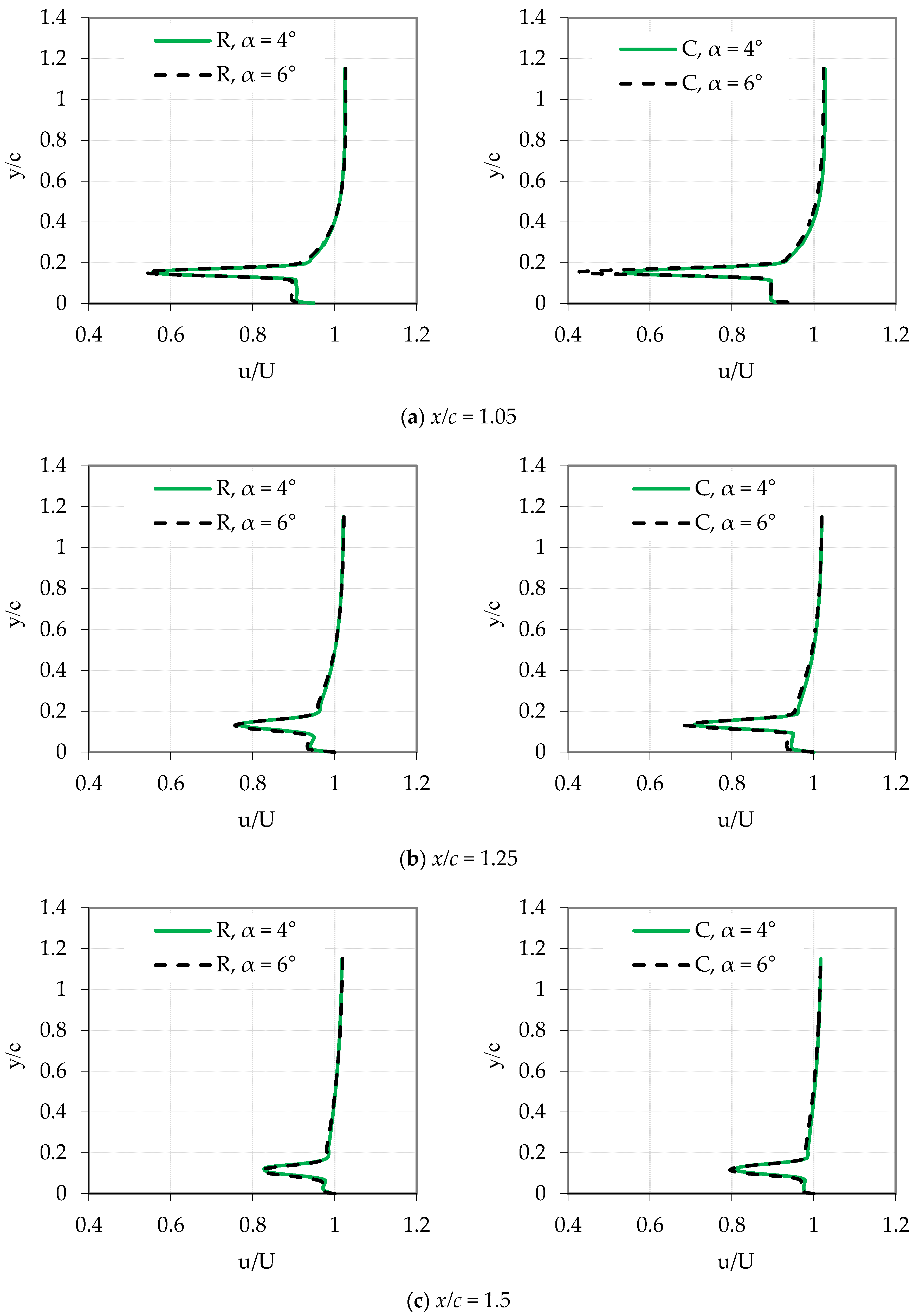
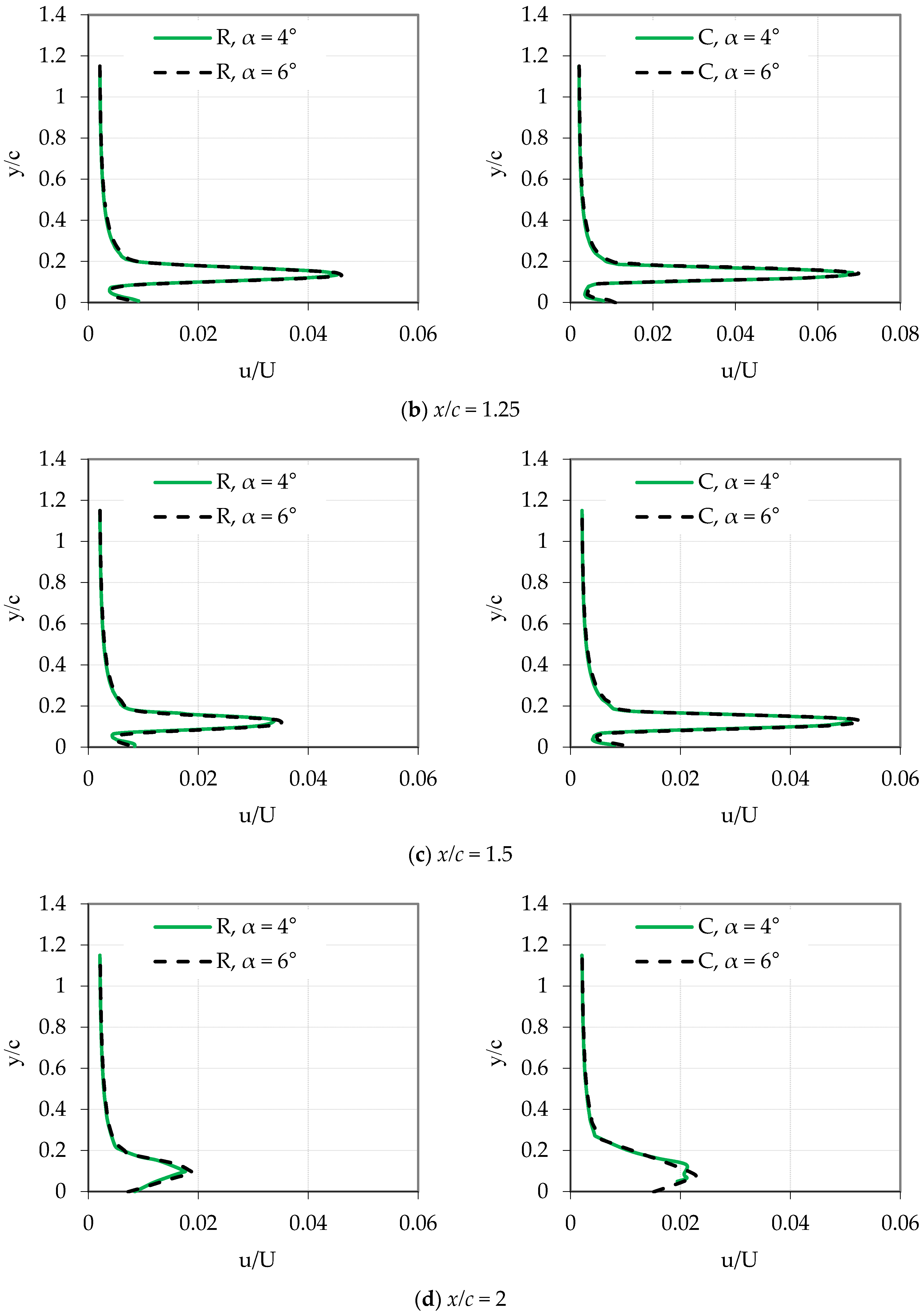
The turbulence intensity and mean velocity releases were obtained in the wake region in the back of the compound wing and the rectangular wing at four axial directions (x/c = 1.05, 1.25, 1.5, 2) from the ground until y/c = 1.15. The reference frame for the coordinates of x and y was the leading edge and the ground surface, respectively. Figure 10 and Figure 11 illustrate the comparisons of the wake region between a present compound wing and a common rectangular wing at a ground clearance of 0.15 and two attack angles at 4° and 6°. These comparisons present the maximum defect velocity, the width of the wake region, and the peak of turbulent intensity.

Figure 10a shows the velocity distribution at x/c = 1.05 and h/c = 0.15 behind both wings. For the compound wing, the velocity defect had a considerable increase; when the angle of attack was enhanced from 4° to 6°. However, for the rectangular wing, only a small variation was recorded. The velocity deficiency in the wake region in the back of the compound wing was noticeability greater than that of the rectangular wing, where the maximum defects for compound and rectangular wings at the angle of attack of 6° were 57% and 46%, respectively, as shown in Figure 10a. As mentioned previously, this higher defect was due to the lower momentum when the airflow left the trailing edge of the compound wing. The thickness of the wakes of both wings had a slight increment with the augmented of the angle of attack, which was around 0.6 times of the chord-wise of the wings (60 mm). The maximum velocity deficiency (d_e) has been calculated as follows:

$$d_e=(1-\frac{u}{U})\times 100.$$

(17)

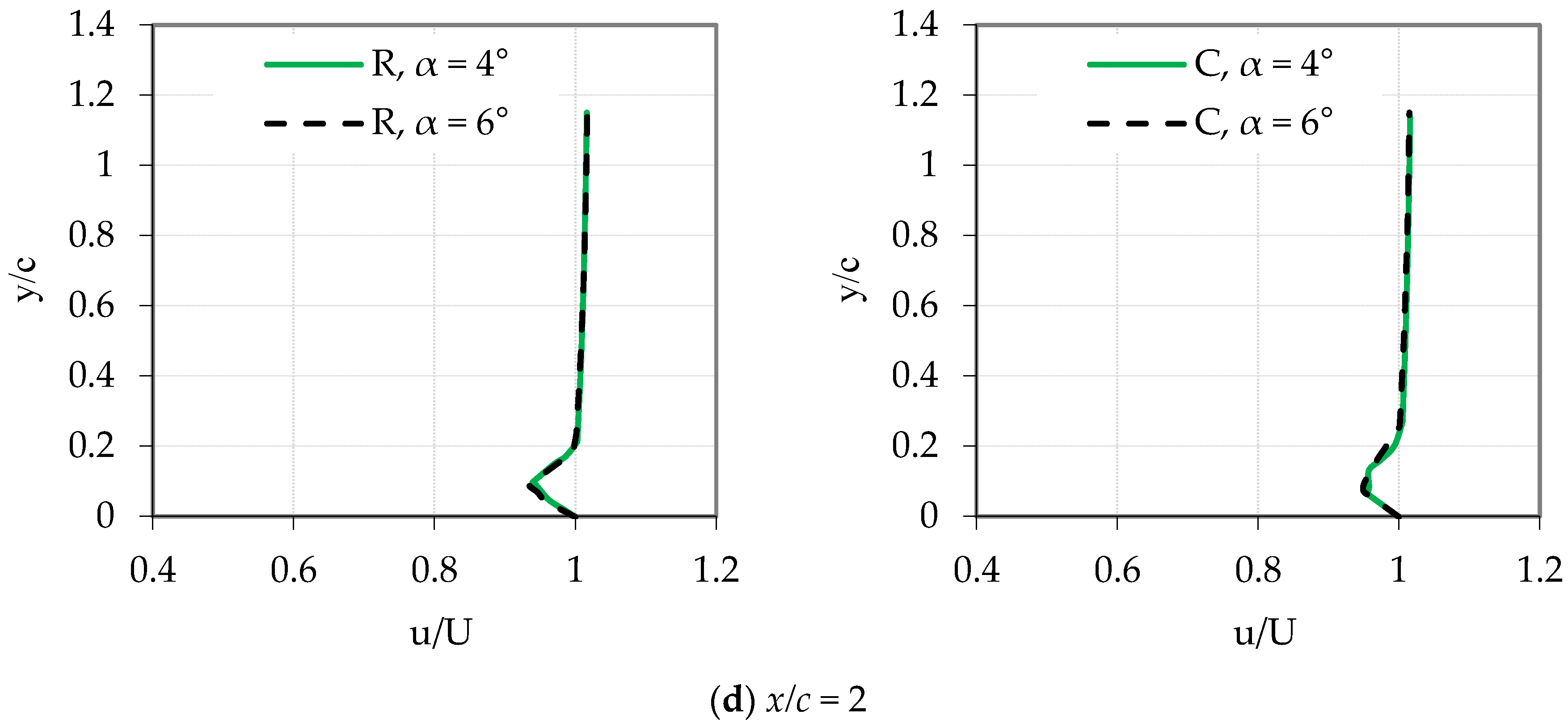
Generally, the defect of the velocity and thickness of the wake region decreased with increasing axial distance from both wings (Figure 10a–d). The maximum velocity defect for both wings at the angle of attack of 6° is shown in

Table 3. Maximum velocity deficiency in the wake area in the back of the compound and the rectangular wing.

x/c	Compound Wing		Rectangular Wing
	α = 4°	α = 6°	α = 4°	α = 6°
1.05	46%	57%	44%	46%
1.25	29%	32%	23%	25%
1.5	19%	20%	17%	18%
2.0	4%	5%	6%	7%

. The velocity defect of the compound was higher until 1.5 c from the leading edge (75 mm from the trailing edge) when the axial distance built up.

Hence, there were little differences between the two wings. The location of the greatest velocity deficiency of both wings was approximately similar. For the adjacent trailing edge, it (y/c) was approximately similar to the ground clearance (h/c = 0.15) of the wings, as shown in Figure 10a. This position reached the ground surface; thus, the axial distance from the trailing edge was enhanced (Figure 10a–d).

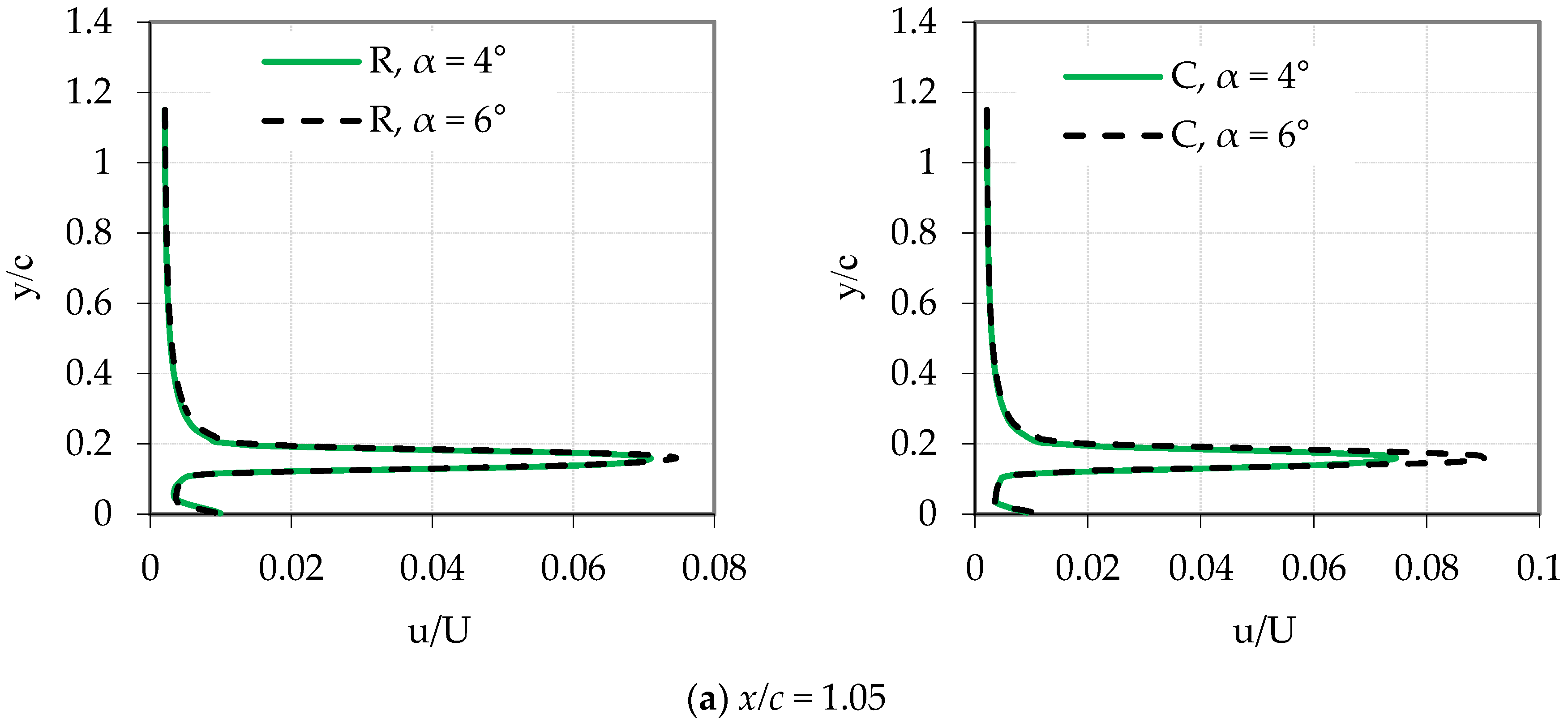
Flow turbulence behind the wings at the ground clearance of 0.15 and two attack angles of 4° and 6° are displayed in Figure 11. The turbulence level of both wings was augmented in the ground effect; therefore, the attack angle increased. At both attack angles, the peak of turbulent intensity for the compound wing was significantly more, particularly at x/c = 1.05 and an attack angle of 6° (Figure 11a). The peaks of turbulence are sorted in

Table 4. The maximum turbulent intensity in the wake region in the back of the compound wing and the rectangular wing.

x/c	Compound Wing		Rectangular Wing
	α = 4°	α = 6°	α = 4°	α = 6°
1.05	7.4%	9%	7%	7.4%
1.25	6.8%	7%	4.5%	4.6%
1.5	5.1%	5.3%	3.4%	3.5%
2.0	2.1%	2.3%	1.8%	1.9%

for the angle of attack of 6°. In addition, the position of this peak near the trailing of both wings was close to the ground clearance, and moved to the ground with the increment of axial distance (x/c).

7. Conclusions

The present research numerically evaluated the flow around and behind a compound wing and a rectangular wing of Wing-in-Ground effect vehicles at various angles of attack working in-ground-effect. The pressure scattering on the compound wing’s surface and detailed exploration of the wake region behind the wings by means of velocity and turbulent intensity are performed. The main outcomes of this analysis are synthesized, as in the following:

(1)

The validation process of the simulation results for the compound wing reveals that the lift-to-drag ratio results are substantially validated, instead of the drag coefficient validation being achieved only for the lower angles of attack. This means a shortcoming in the modelization of the RANS approach in particular, due to the strong gradient of pressure and velocity near to the ground-wall (i.e., at a high angle of attack).

(2)

The recorded positive pressure on the lower surface of the compound wing was noticeably tougher than that of the rectangular wing. However, the suction effect on the upper surface of the rectangular wing was slightly higher.

(3)

At a lower attack angle, negative pressure was observed on the lower surface of the rectangular wing, whereas positive pressure was detected on the lower surface of the compound wing.

(4)

The adverse pressure gradient was higher on the upper surface of the compound wing. The effect of the attack angle of the compound wing on the turbulence level and velocity distribution was higher in the wake area.

(5)

The velocity defect and turbulent intensity near the trailing edge of the compound wing were depicted greater than that of the rectangular wing. However, these differences were reduced as the axial position behind the wings increased.

(6)

The positions of the maximum of velocity defect and turbulence level were near the ground behind the trailing edge of the wings, and this position dropped with enhanced axial distance from the trailing edge.

Hence, this research represents a contribution for the WIG designers in order to evaluate the no-standard (compound) wing geometry combining CFD simulations and experimental output.

8. Recommendations for Future Work

The current work only illustrated in-depth investigation on the present compound wing for various attack-in-ground effect angles. To achieve the next objective and to reply to a recent call for research, the effect of ground clearance, as well as Reynolds number with a higher range of angles of attack and flow structure around and behind the compound wing, will be investigated. In addition, different types of NACA airfoil section or Clark-Y section are needed to examine this extended study. This can deliver useful data on the present wing for researchers and designers.