Abstract
To calculate the environmental capacity of the estuaries of Haizhou Bay in northern Jiangsu, China in 2006 and 2016, this study employed the share ratio approach and established a tidal hydrodynamic model and a water quality diffusion model by the Delft 3D software to perform the numerical simulation. The article compared the environmental capacity in 2006 and 2016, and analyzed the changes between these years. The scenario analysis method was used to explore the influence of factors on the environmental capacity and quantify the contribution of each influencing factor. The results show that the theoretical environmental capacity was reduced by 32.718 tons/day (28.56%) from 114.571 tons/day in 2006 to 81.853 tons/day in 2016. The remaining environmental capacity was reduced by 6.955 tons/day (56.92%) from 12.219 tons/day in 2006 to 5.264 tons/day in 2016. The changes in topography and the amount of runoff into the ocean through the estuaries of Haizhou Bay between 2006 and 2016 reduced the total environmental capacity of the estuaries by an influence ratio of 0.363:0.637. The study will provide the management of the marine environment of Haizhou Bay with information to control the aggregate pollutants flowing into the ocean and support the social and economic sustainable development of Haizhou Bay.
1. Introduction
The ocean is the most low-lying area on the Earth, and land-based pollutants correspondingly end up flowing into the ocean under the influence of gravity. Humans have caused increasingly severe ocean pollution as the economy of coastal areas develops and urbanization accelerates [1,2,3]. The land-based domestic and production sewage brought by the rivers flowing into the ocean has placed a considerable pressure on coastal waters, reducing their water quality, and it may even affect threatened bird habitats [4,5].
As marine development activities gained momentum in recent years, marine pollution has become increasingly serious and impeded the development of coastal areas. To realize sustainable development of coastal areas, it is necessary to accelerate the treatment and restoration of the marine water environment while developing and utilizing marine resources. Therefore, both the government and academics are trying hard to find effective measures to balance marine development and protection. One traditional measure for marine water environment management is limiting the discharge of pollutants. The main pollutants in the coastal waters are mostly from rivers or sewage outlets. For many years, the government, with a vision to protect the water environment, has set limits on discharges of pollutants. Though most coastal areas have controlled the discharges effectively, the offshore seawater quality has not improved, and the total discharge has kept rising. This implies that setting limits on the discharge of pollutants alone is far from enough. First of all, both the river runoff and the discharges from sewage outlets play a decisive role in the total discharge of pollutants, and the increase of the total discharge will worsen the marine environment. Besides, pollutant discharge control often only considers the impact of a single discharge outlet but ignores the superposition of pollutants discharged from multiple outlets in a region. Thus, controlling the discharge of pollutants alone will not be effective in improving the quality of coastal waters or achieving the goal of marine environment protection.
The ocean has a remarkable self-purification capacity and can accommodate tons of pollutants, and transfer, dilute, degrade, and purify pollutants through physical, chemical, and biological actions. It cannot, however, accommodate an unlimited burden of pollutants. The marine environmental capacity refers to the maximum amount of environmental pollutants that can be released into the ocean within a certain period of time to maintain the water quality standard required by specific ecological and environmental functions of a certain water body. Some scholars also call it total maximum allocated load (TMAL) [6]. When the aggregate pollutants released into the ocean are below this capacity, the ocean’s self-purification capability keeps the ocean environment healthy. However, when the aggregate pollutants discharged exceed the upper limit of the marine environmental capacity, both the marine environment and the marine functions will be damaged, and may never fully recover [7]. The traditional approach to managing the marine water environment is prevention and control with a focus on limiting the discharge concentration of pollutants. Most of the main pollutants in coastal waters are discharged into the neighboring waters through rivers flowing into the ocean or sewage outlets. For many years, the water environment has been protected by meeting the standards for discharge concentration, and the pollutant concentration has been controlled. However, the quality of coastal waters has not been improved, and the aggregate discharge of pollutants has continued to increase. A more effective way to manage and control the marine environment may be to determine the marine environmental capacity and use this metric as a basis for controlling the aggregate pollutants discharged into the ocean in a rational way.
In 1986, the Group of Experts on the Scientific Aspects of Marine Environmental Protection (GESAMP) formally defined the concept of environmental capacity: environmental capacity is the characteristic of the environment, and the capacity of the environment to accommodate certain substances on the premise that it will not cause intolerable impact on the environment [8]. The research on marine environmental capacity started earlier outside China. For example, Krom et al. have estimated the environmental capacity of Haifa Bay on the Mediterranean coast of Israel [9]. Nam et al. evaluated the environmental capacity of Woosedo Island off the southwest coast of South Korea [10]. In these years, scholars have focused on the impact of the deterioration of the marine environment on marine life, and explored comprehensive measures for the management of marine ecology. Pandolfi et al., for example, studied the decline of corals around the world [11]. Trela et al. studied the comprehensive management of the Baltic Sea in Sweden [12]. To date, research on the marine environmental capacity in China has largely focused on comparing different methods and on reducing excessive discharges to meet relevant regulations and standards. Some scholars have examined rational ways to reduce pollutant discharge [13], whereas others have explored more accurate ways to calculate the marine environmental capacity of a specific pollutant and thus better control the aggregate discharge of pollutants [14]. Therefore, scientific and reasonable determination of marine environmental capacity has become a hot topic in marine environmental research. Despite the many studies devoted to this field over these years, a universal calculation method has not yet been found, but different methods have been developed for specific coastal areas. There are two kinds of methods for calculating marine environmental capacity. One method is to study the influence of tidal flow and other factors on pollutants, and use mathematical model to calculate the results of environmental capacity, such as sharing rate method [15,16,17,18], optimization method [14,19] and model trial calculation method [20,21,22]; the other method is to collect detailed environmental monitoring data, and obtain the results of environmental capacity through data processing, analysis and calculation, such as box model method [23,24,25] and GIS method [26,27]. Few studies, however, have considered the changes and influencing factors of environmental capacity. Relevant studies are focused on rivers and lakes [28,29], and analysis of the impact of changes in water quality, flow, or amount of water flowing into lakes on the environmental capacity [30,31]. The values of environmental capacity under different circumstances are calculated separately based on different water quality and flows [16,32]. The trends of influence of the myriad factors on the environmental capacity are typically qualitatively analyzed without quantitatively calculating the contribution rates of these factors [33,34]. Research into changes of marine and water environmental capacity has mainly focused on the differences in environmental capacity under different water quality and hydrological conditions, as well as the impact of land reclamation projects on the environmental capacity of bays [35,36]. The study of factors causing changes in environmental capacity is relatively simple, without taking into account the possible superposition effects of multiple factors. Moreover, when examining the factors influencing changes in environmental capacity, previous studies have only focused on qualitative analysis of the trends of influence [15,23], without a quantitative assessment on related coverage concerning the preceding factors.
Haizhou Bay, situated in the northernmost section of Jiangsu province, boasts the richest marine resources in Jiangsu province, China. This coastal area accommodates diverse and intensive development activities, including pond culture, open-water aquaculture, tourism and entertainment, industrial use of sea, sea for land reclamation, and sea for sewage and dumping. Between 2006 and 2016, the area of land reclamation for industrial and urban construction in Haizhou Bay totaled 43.4 km2. In addition, nine rivers in Haizhou Bay flow into the ocean, bringing pollutants from land-based and domestic sewage sources, which damages the coastal environment of Haizhou Bay. According to the report for 2017 Lianyungang Bulletin on Marine Environmental Quality, the water quality in 60.18% of the total area in Haizhou Bay was rated Class I and Class II, whereas water in 39.82% of the total area was rated as Class III. The polluted areas are mainly in the coastal waters, particularly the estuaries. Monitoring results of water quality of main rivers flowing into the ocean in Lianyungang City in 2017 showed that 79.5% of these river samples were poorer than the Class V water quality standard for surface water, with the main pollutants being chemical oxygen demand (COD) emissions, ammonia nitrogen, total phosphorus, and petroleum. Protecting the marine environment of Haizhou Bay and striking a balance between development and protection are important for sustainable development of Haizhou Bay.
At present, the research on marine environmental capacity mainly focuses on the calculation of total emission of pollutants based on the current situation, but few on the variation and mechanism of marine environmental capacity. This study analyzed the changes in the coastline of Haizhou Bay as well as the runoff and water quality of rivers flowing into the ocean in this area. The environmental capacity of the coastal estuaries of Haizhou Bay was calculated in different periods through numerical simulation based on data such as coastal topography, changes in the coastline, runoff of the rivers flowing into the ocean, and the water quality of the river water. Scenario analysis was used to examine the extent to which factors such as the runoff of rivers flowing into the ocean, land reclamation, and river water quality affects the changes in marine environmental capacity in Haizhou Bay. We assumed that one factor in the amount of sewage or topography remains unchanged, and calculated the environmental capacity of a certain scenario. Then we compared it with the actual environmental capacity in order to calculate the influence ratio of each factor on the environmental capacity. These findings will provide a reference for similar future studies, and the management of the marine environment of Haizhou Bay to control the aggregate pollutants flowing into the ocean and support the social and economic sustainable development of Haizhou Bay.
2. Materials and Methods
2.1. Overview of the Study Area
Haizhou Bay, Lianyungang is located in the northeast of Jiangsu province, China, and to the south of Shandong province. It is the westernmost open bay in the south Yellow Sea of China, covering an area of around 820 km2. It ranges from Lanshan Town in Rizhao City, Shandong province in the north (Point A in Figure 1: 35°05′55″ N, 119°21′53″ E), to Gaogong Island in Lianyun District, Lianyungang City, Jiangsu province (Point B in Figure 1: 34°45′25″ N, 119°29′45″ E) in the south. The coastline of the study area is 130.3 km in length. The majority of Haizhou Bay is governed by Lianyungang City, Jiangsu province, and its adjacent administrative districts are Ganyu County and Lianyun District of Lianyungang City. There are nine main rivers in Haizhou Bay (Figure 1). Longwang River flows into Haizhou Bay via Longwang estuary, Xingzhuang River into Haizhou Bay via Xingzhuang estuary, Shangwang River into Haizhou Bay via the barrage of Shangwang River, Qingkou River into Haizhou Bay via the barrage of Qingkou River; the rest five rivers, i.e., Zhuji River, Fanhe River, Xinshu River, Qiangwei River, and Dapu River, converge in Linhong Estuary, and thus all flow into the ocean via Linhong Estuary. Therefore, the nine rivers in the studied waters have five major estuaries. The length and drainage area of main rivers in Haizhou Bay are shown in Table 1.
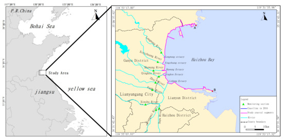
Figure 1.
The location of study area.

Table 1.
The length and drainage area of main rivers in Haizhou Bay.
2.2. Data Sources and Analytical Method
Remote-sensing image interpretation of the LANDSAT images of 2006 and 2016 was carried out through ENVI to determine the coastlines of the research area in the two years, so that the sea reclamation projects from 2006 to 2016 can be analyzed.
The 1:25,000 topographic mapping of Haizhou Bay Sea area in 2006 and 1:20,000 topographic mapping of the area in 2016 were collected. Based on the topographic maps in different time periods, the changes of topographical erosion and deposition in Haizhou Bay were compared and analyzed.
The ownership data of marine development and utilization in 2006 and 2016, as well as marine spatial planning, were collected. ArcGIS was used for data processing and integration, information superimposition, spatial analysis, and the output vector data about the coastal development, submarine topography, and marine spatial planning data for 2006 and 2016. According to the hydrological data from Hydrology and water resources survey Bureau of Jiangsu Province and “Lianyungang Coastal Water Pollution Control Program”, the runoff and the monthly average COD emission concentration of Haizhou Bay in 2006 were obtained.
According to the monitoring data of Lianyungang Rivers into the sea in 2016 provided by Lianyungang Environmental Protection Bureau, the monthly average COD emission concentration and the runoff of main rivers in Haizhou Bay in 2016 were obtained.
2.3. Research Method for Environmental Capacity Estimation
2.3.1. Share Ratio Approach
The share ratio approach was used to build a model for concentration diffusion of pollutants discharged into the ocean based on the investigation of pollution sources and the monitoring of water quality. The share ratio field and response coefficient field of each point source were obtained through numerical simulation, alongside the environmental capacity of pollutants discharged into the ocean according to the targets of water quality and the existing concentration. The sharing ratio method is a total amount control method, which is used to calculate the environmental capacity of estuaries or sewage outlets in order to control the total emission of land-based pollutants.
First, an input–response relationship between the pollution source and the receiving water should be established, which is the key to the control over the aggregate discharge of pollutants. If the hydrodynamic conditions of a certain water body and the discharge and location of the coastal sewage outlets remain unchanged, the concentration field formed by the pollution source at a certain location will also remain unchanged, indicating an unchanged response relationship. The periodic averages of pollutant concentration and response should be used. Based on the principle of linear superposition, the concentration field formed by interactions of multiple pollution sources in a specific water body can be deemed as the linear superposition of the concentration field produced by the individual influence of each pollution source. According to these response relationships, the maximum allowable aggregate discharge of each sewage outlet can be calculated by taking the standards for water quality as constraints.
The response relationship ai (x, y) between each discharge source and the receiving water is established, so the concentration field Ci (x, y) formed by separate discharge of each point source can be treated as a multiple of the response coefficient field, which means that:
where Qi is the source intensity of the ith pollution source; ai (x, y) is the response coefficient, namely the response coefficient field formed when Qi = 1, which represents the response relationship of water quality in the water to a certain point source and is the basis for study of environmental capacity; and (x, y) is a spatial point coordinate.
The convection–diffusion equation can be taken as a linear equation given that the flow velocity and diffusion coefficient are known, which satisfies the superposition principle. The equilibrium concentration field formed by interactions of multiple pollution sources is, therefore, the linear superposition of the concentration field formed by each pollution source at its own existence, written as follows:
The share ratio can be defined as the share (percentage) represented by the influence of each pollution source to that of all pollution sources in the waters, reflecting the contribution rate of a certain pollution source to the overall pollution of the waters. The share ratio is calculated as follows:
where Cs (x, y) is set to the water quality standard of the waters. If the share ratio field of the same pollution source is assumed to be unchanged, the share ratio concentration of the ith point source under the water quality standard is met:
By taking into account the response relationship of the ith point source, we obtain:
The allowable discharge Qsi of the ith point source that meets the target for water quality (the marine environmental capacity) is then obtained:
The discharge of pollutants should be reduced if the existing discharge is greater than the allowable one. The marine environmental capacity has not reached its limit if the existing discharge is less than the allowable one.
2.3.2. Numerical Simulation
The underlying idea of the share ratio approach is the diffusion concentration field formed after pollutants are diffused from the discharge outlet, from which the response coefficient of pollutants is extracted and calculated using a diffusion model for water quality. A model for tidal hydrodynamics of Haizhou Bay was constructed with the numerical simulation software Delft 3D to simulate the tidal field of Haizhou Bay. On this basis, the model for material transport was applied to create a diffusion model for water quality. The marine environmental capacity of the estuaries of Haizhou Bay at different times could be calculated based on the model for tidal hydrodynamics, the diffusion model for water quality, and the share ratio.
Delft 3D Model
(1) Basic principles
Delft3D is a multidimensional (2D, 3D) hydrodynamic (and mass transport) simulation program [37,38,39,40]. It calculates unsteady flow by establishing linear or curvilinear grids suitable for boundary conditions. Based on the Navier Stokes equation, it uses the alternating direction implicit method (ADI) of finite difference method. The governing equations in the corresponding coordinate system are discretized.
(2) The governing equation
Hydrodynamic governing equation is expressed as follows.
The pollutant diffusion equation is expressed as follows.
In the formula, t is time; u and v are velocity components along x and y direction, respectively; h is the distance from the seabed to the stationary sea surface, that is, the still water depth; ζ is the fluctuating water level upward from the stationary sea surface; f is the Coriolis parameter; g is the acceleration of gravity; τbx and τby are the components of the bottom shearing stress in x and y directions under the action of wave and current, respectively; Ex and Ey are the horizontal turbulent viscosity coefficients in X and Y directions, respectively; Sxx, Sxy, Syx and Syy are wave stresses in each direction. C is the concentration of the substance; Kx and Ky are turbulent diffusion coefficients in X and Y directions, respectively; fc is the pollution intensity of pollution source.
(3) Definite solution condition
i. Hydrodynamic equation
The initial conditions:
In the above formula, u0, v0 and ζ0 are the tide level and velocity at the beginning of model calculation. t is the initial calculation time of the model.
Boundary conditions:
In the sea area of the study area, the model adopts the tidal level boundary on the open boundary : .
The tide level is calculated according to the large-scale tidal wave model in the South Yellow Sea. On the closed boundary : Normal velocity = 0, where n represents the outer normal of the boundary.
ii. Pollutant diffusion equation
The initial conditions:
Boundary conditions:
There is no flux at the closed boundary, so the concentration is set at 0. On the open boundary, when the flow direction of tidal current is outward, must be satisfied. If the flow direction is inward, the boundary value is 0.
Model Grid and Parameter Setting
Based on the topography and tidal hydrodynamic characteristics of Haizhou Bay in Lianyungang, the grid was drawn. The numerical simulation of tidal current field in Haizhou Bay is realized by constructing large-scale model and small-scale model nesting. The large-scale model is a large-scale tidal current wave movement model in the South Yellow Sea of China, including the coastline of Jiangsu Province. The model ranges from Shandong to Zhejiang, including the entire Jiangsu coast, Yangtze River Estuary and Hangzhou Bay. The boundary tidal level data of the small-scale model is obtained from the calculation results of the large-scale model. Then the tidal current model of Lianyungang Coastal area can be established. The model ranges from Lanshan District in Rizhao city, Shandong Province to Zhongshan Estuary in Xiangshui County, Yancheng City, Jiangsu Province. It covers the whole coastal area of Lianyungang, as shown in Figure 2.
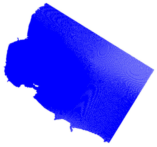
Figure 2.
Grids for numerical simulation calculation.
The Lianyungang area, spanning 113 km from north to south and 120 km from east to west, is taken as the scope for model calculation in this paper. Within this scope, the northwest and southwest boundary are the fixed boundary of Lianyungang land. The northeast and southeast boundaries are the open boundaries of the sea area. The control method of boundary conditions is tidal level control. Orthogonal grids are used to draw the model. There are 387,325 grid cells in the model. In the process of grid drawing, the sea area of Haizhou Bay is encrypted. The smallest grid cell is 82 m × 69 m. The Manning coefficient is 0.02. The initial concentration of COD is set to 0. The water temperature is 5 °C. The annual average wind speed is 5.5 m/s, and the normal wind direction is east.
Model Validation
This paper studies the changes in the environmental capacity of Haizhou Bay from 2006 to 2016. Therefore, in the calculation and validation of the model, the relevant data matching the research time is used. When calculating the marine environmental capacity in 2006, the coastline, seabed topography and hydrological data in 2006 were used for numerical simulation. When calculating the marine environmental capacity in 2016, corresponding data of the study area in 2016 were used for numerical simulation.
(1) Verification station
According to the measured data of Hydrology Bureau of Changjiang Water Conservancy Commission in 2006, the results were verified. The whole course of hydrological survey is from 2 January to 9 January 2006. The calculated time step is 0.5 min. The verification includes tide level verification and tidal current verification. The feasibility of numerical simulation is verified by comparing the measured data with the calculated results of numerical simulation. In this paper, three tide stations are selected. They are M1 station of Lanshan Port, M2 station of Lianyungang oil supply station and M3 station of Xiaodinggang, as shown in Figure 3a. According to the sea area studied in this paper, nine tidal current verification points are selected. The locations are shown in Figure 3a.
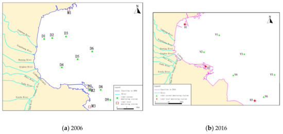
Figure 3.
Locations of verification tide level and current monitoring stations in 2006 and 2016.
The data from the hydrologic survey carried out by Tianjin Water Transport Engineering Survey and Design Institute in the sea area of Haizhou Bay were used for verification. The whole course of hydrological survey is from 23 January 2015 to 29 January 2015. In this paper, three tide stations are selected. They are H1 station in Ganyu port area, H2 station in east-west connecting island and H3 station in Kaishan island. The locations of these six tide stations are shown in Figure 3b. Six tidal current measurement points in the waters near Lianyungang were selected for tidal current verification. The locations are shown in Figure 3b.
(2) Verification results
The results of tide level verification in 2006 are shown in Figure 4. Figure 5 shows the comparison between the measured and calculated values of nine tide stations in 2006.
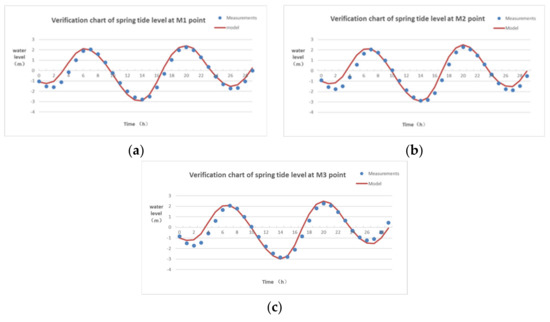
Figure 4.
Tide level verification in 2006. (a) Verification chart of spring tide level at Point M1; (b) Verification chart of spring tide level at Point M2; (c) Verification chart of spring tide level at Point M3.
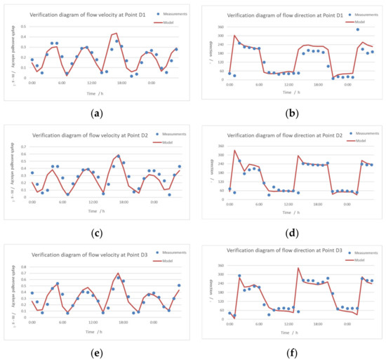
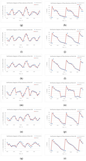
Figure 5.
Tide current verification in 2006. (a) Verification diagram of flow velocity at Point D1; (b) Verification diagram of flow direction at Point D1; (c) Verification diagram of flow velocity at Point D2; (d) Verification diagram of flow direction at Point D2; (e) Verification diagram of flow velocity at Point D3; (f) Verification diagram of flow direction at Point D3; (g) Verification diagram of flow velocity at Point D4; (h) Verification diagram of flow direction at Point D4; (i) Verification diagram of flow velocity at Point D5; (j) Verification diagram of flow direction at Point D5; (k) Verification diagram of flow velocity at Point D6; (l) Verification diagram of flow direction at Point D6; (m) Verification diagram of flow velocity at Point D7; (n) Verification diagram of flow direction at Point D7; (o) Verification diagram of flow velocity at Point D8; (p) Verification diagram of flow direction at Point D8; (q) Verification diagram of flow velocity at Point D9; (r) Verification diagram of flow direction at Point D9.
The results of tide level verification in 2016 are shown in Figure 6. Figure 7 shows the comparison results of measured and calculated values of six tidal current stations in 2016.
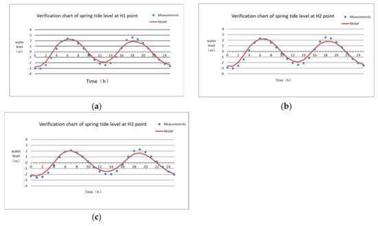
Figure 6.
Tide level verification in 2016. (a) Verification chart of spring tide level at Point H1; (b) Verification chart of spring tide level at Point H2; (c) Verification chart of spring tide level at Point H3.
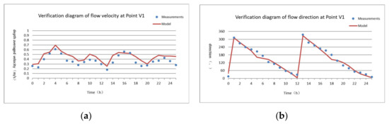
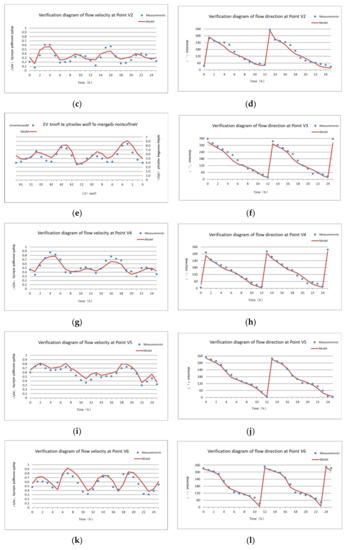
Figure 7.
Tide current verification in 2016. (a) Verification diagram of flow velocity at Point V1; (b) Verification diagram of flow direction at Point V1; (c) Verification diagram of flow velocity at Point V2; (d) Verification diagram of flow direction at Point V2; (e) Verification diagram of flow velocity at Point V3; (f) Verification diagram of flow direction at Point V3; (g) Verification diagram of flow velocity at Point V4; (h) Verification diagram of flow direction at Point V4; (i) Verification diagram of flow velocity at Point V5; (j) Verification diagram of flow direction at Point V5; (k) Verification diagram of flow velocity at Point V6; (l) Verification diagram of flow direction at Point V6.
The verification curve in the figures show that the calculation results of tide level coincide well with the measured values in 2006 and 2016, and there is little difference between the duration of rising and falling tides. The calculated results of the model coincide well with the measured values of tidal current in 2006 and 2016. This means that the model can better reflect the actual situation, and can accurately predict the hydrodynamic characteristics of the sea area near Lianyungang.
2.3.3. Setting of Boundary Conditions for Calculation and Scenario Simulation
According to the share ratio method, the marine environmental capacity of the estuary area in 2006 and 2016 can be calculated by the Delft 3D numerical simulation method based on the landside coastline boundary (actual bathymetric topography), hydrodynamic conditions and the discharge conditions of the nearshore estuary respectively in 2006 and 2016.
In 2006 and 2016, the runoff and pollutant concentration of the rivers entering the sea changed, and the estuary topography and land boundary also changed due to offshore sea reclamation projects, so the estuary marine environmental capacity in 2016 and 2006 was bound to change as well.
In order to quantify the impact of topography and river discharge on the marine environmental capacity of estuaries, two computational boundaries and scenarios were assumed.
Scenario A: The marine environmental capacity under the land-side boundary conditions of the coast of Haizhou Bay in 2006 and the discharge conditions of the coastal estuaries of Haizhou Bay in 2016 (topography in 2006 + estuaries in 2016).
Scenario B: The marine environmental capacity under the land-side boundary conditions of the coast of Haizhou Bay in 2016 and the discharge conditions of the coastal estuaries of Haizhou Bay in 2006 (estuaries in 2006 + topography in 2016).
Scenarios A and B assume that only one condition of the topography and river discharge has changed from 2006 to 2016. The mathematical model is used to calculate the environmental capacity of the estuary under the conditions of Scenario A and Scenario B. Then, by comparing hypothetical Scenarios A and B with the actual environmental capacity in 2006 and 2016, the impact of topography or a single factor of river sewage discharge on the estuary environmental capacity can be quantified.
The difference between Scenario A and 2006 estuary environmental capacity reflects the impact of river discharge amount changes on the environmental capacity; while the difference between 2016 estuary environmental capacity and Scenario A reflects the impact of topographic changes on the estuary environmental capacity.
The difference between Scenario B and the estuary environmental capacity in 2006 reflects the impact of topographic changes on the environmental capacity, while the difference between Scenario B and the estuary environmental capacity in 2016 reflects the impact of river pollutant discharge changes on the estuary environmental capacity.
3. Results
3.1. Changes in Natural Conditions
Between 2006 and 2016, Haizhou Bay coastline extended in length from 106.2 to 130.3 km, an increase of 24.1 km (Figure 8), and some sections moved eastwards as a result of human activities.
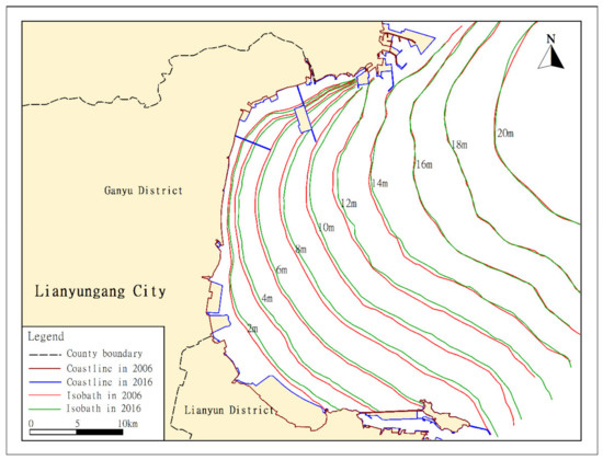
Figure 8.
Changes of coastline and isobath in Haizhou Bay from 2006 to 2016.
Owing to sea-enclosure marine culture, marine reclamation land for ports and Binhai New City from 2006 to 2016, the sea area for tidal prism decreased. Meanwhile, the intensity, density, and coverage of coastal development of Haizhou Bay drastically increased. The area of sea reclamation over these ten years is 34.9 km2.
A comparison of isobaths between 2006 and 2016 shows that, the isobath lines of 16, 18 and 20 m basically coincided. It shows that there was little change in the terrain of Haizhou Bay below 16 m. There is a considerable terrain change in the sea areas shallower than 16 m. On average, isobaths from 2 m to 14 m of Haizhou Bay moved outwards by 350 m from 2006 to 2016(Figure 2). The change of isobath shows that the sea area above the 16 m isobath is still in the silting state, and the sea area below the 16 m isobath is basically stable.
A comparative analysis of the changes in the rivers into Haizhou Bay from 2006 to 2016 (Table 1) demonstrates that the runoff of the nine rivers decreased by 451,233 m3/ day. The water quality of Longwang River and Qingkou River was basically stable with slight deterioration. The water quality of Xingzhuang River, Zhuji River, Fanhe River, decreased significantly, whereas that of Shawang River, Xinshu River, Qiangwei River, and Dapu River improved (Table 2).
Table 2.
The amount of runoff and chemical oxygen demand (COD) concentration of the nine main rivers in Haizhou Bay from 2006 to 2016.
3.2. Determination of Calculation Boundary
The development activities of the waters outside the estuaries of Haizhou Bay are dominated by open-water aquaculture (Figure 9). The water quality of the culture area should meet the requirements for water quality standard for Class II seawater of the Marine Functional Zoning of Lianyungang City. To ensure that the environmental water quality of the mariculture area in Haizhou Bay is not lower than Class II, we selected the sensitive points closest to the coast of Haizhou Bay and of the five major estuaries as the control points of water quality for the share ratio approach based on mariculture data for 2016. Moreover, COD was selected as the factor for calculating environmental capacity of the estuaries. The COD concentration of the control points should satisfy the requirements for water quality standard for Class II seawater (≤3 mg/L).
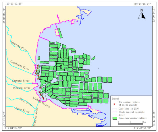
Figure 9.
The control points of water quality.
3.3. Environmental Capacity of the Estuaries in 2006 and 2016
In line with the theoretical basis of the share ratio approach, the pollutant concentration of the control point corresponding to each river flowing into the ocean was calculated based on unit discharge through Delft 3D numerical simulation. The response coefficient of each river flowing into the ocean was calculated with Formula (1), and the share ratio was obtained by considering the actual discharge flux of pollutants of each river. The corresponding environmental capacity was then calculated with Formula (6).
3.3.1. Response Coefficient
Using the Delft 3D software, we calculated the response coefficients of water quality in the control points of the five estuaries in 2006 and 2016. When the coefficient is below 0.0001, we assume that the water quality in the control point was not affected by pollutants. The influence of diffusion on each estuary is shown in Table 3.
Table 3.
The response coefficient of the coastal estuaries in Haizhou Bay in 2006 and 2016.
It can be observed that in 2016, the control points 10 and 11 were affected by the diffusion of pollutants from one river flowing into the ocean only. The remaining control points were affected by the diffusion of pollutants from two or more rivers flowing into the ocean.
In all five estuaries, the number of control points affected by pollutant dispersion increased compare 2016 with 2006. The locations of these 11 control points are fixed, the more control points affected by diffusion, the greater the response coefficient. This shows that the diffusion of pollutants in 2016 was wider and farther than that in 2006. The parallel diffusion along the coast was changed to diffusion towards the ocean away from the shoreline. Reclamation projects have been carried out in the nearshore between Xingzhuang estuary, Shawang estuary and Qingkou estuary in 2016 compared with 2006.The reclamation project affected the velocity and direction of flow in the near shore estuary area. The reclamation makes the velocity of the estuary decrease, and made the water flow out to the outer sea area along the reclamation seawall. The diffusion ability decreases with the decrease of velocity. The influence range and distance of the current into the sea increased, so the number of control points affected by pollutant dispersion increased.
3.3.2. Linear Superposition and Verification
The control points for the water quality target were selected. Specifically, the pollutant concentration in the selected control points should be equal to the prescribed value of the water quality target, and that outside the control points should exceed the prescribed value. Under certain discharge conditions of pollutants, the concentration field where pollutants in the waters are distributed tends to be a stable status. Linear superposition is satisfied between point sources.
Figure 10 presents a comparison of the superimposed discharge and diffusion of the five estuaries in 2006 and 2016. Based on the actual runoff and the concentration, we added the contour lines of the 0.1 mg/L COD concentration after separate discharge by each of the five estuaries, then compared it with the contour lines of the 0.1 mg/L COD concentration after concurrent discharge by the five estuaries. It was found that the superposition of the lines of maximum diffusion of 0.1 mg/L in separate discharge by the five estuaries almost overlapped the unified contour lines after concurrent discharge by the five estuaries. This verifies the pattern of linear superposition for pollutant diffusion under the fixed hydrodynamic field.
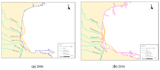
Figure 10.
The comparison of the COD concentration contour lines of separate discharge by the five estuaries and concurrent discharge by the five estuaries of Haizhou Bay in 2006 and 2016.
3.3.3. Share Ratio
The flux of COD pollutants discharged into the ocean was calculated for each river based on the measured COD concentration and runoff of the estuary. The share ratio refers to the percentage of the influence of each pollution source to that of all pollution sources in the waters, reflecting the contribution rate of a certain pollution source to the overall pollution of the waters. The share ratio of each river flowing into the ocean at each control point was calculated and is presented in Table 4.
Table 4.
The share ratio of each river flowing into the ocean at each control point in 2006 and 2016.
3.3.4. Calculation of the Environmental Capacity
The theoretical marine environmental capacity of the coastal estuaries of Haizhou Bay in 2006 and 2016 was then calculated. The remaining environmental capacity was obtained by subtracting the used environmental capacity from the theoretical marine environmental capacity (Table 5).
Table 5.
The marine environmental capacity of COD in 2006 and 2016.
In 2006, the actual daily COD discharged by the main rivers flowing into the ocean in the coastal estuaries of Haizhou Bay in 2006 was 102.353 tons, while their theoretical environmental capacity was 114.571 tons, so the remaining environmental capacity was 12.219 tons.
In 2016, the actual daily COD discharged by the main rivers into Haizhou Bay in 2016 was 76.589 tons, while their theoretical environmental capacity was 81.853 tons, so the remaining environmental capacity was 5.264 tons.
3.4. Calculation Results for the Hypothetical Scenarios
The environmental capacity of COD in seawater under the two calculation boundaries and scenario conditions were calculated separately (Table 6).
Table 6.
The environmental capacity of COD in seawater under t different calculation boundaries and scenario conditions (Unit: ton).
4. Discussion
4.1. Actual Changes Between 2006 and 2016
The environmental capacity of COD in coastal estuaries of Haizhou Bay in 2016 and 2006 is compared in Table 7.
Table 7.
The actual changes in the COD environmental capacity of the coastal estuaries of Haizhou Bay between 2016 and 2006 (Unit: ton).
In 2016, the theoretical environmental capacity of the coastal estuaries of Haizhou Bay was 81.853 tons/day, falling by 32.718 tons/day from 114.571 tons/day in 2006, and this decrease accounted for 28.55% of the environmental capacity in 2006. The theoretical environmental capacity of Xingzhuang River, Qingkou River and Linghong Estuary saw a slight increase of 0.951–1.91 tons/day. In contrast, the theoretical environmental capacity of Longwang River and Shawang River decreased, for example, that of Longwang River plummeted by 36.547 tons/day, representing approximately 86.84% of the environmental capacity of this estuary in 2006.
A comparative analysis of the changes in the coastal estuaries of Haizhou Bay from 2006 to 2016 (Table 1) demonstrates that the water quality of Longwang River and Qingkou River was basically stable with slight deterioration. The water quality of Xingzhuang River decreased significantly, whereas that of Shawang River and Linhong Estuary improved. The runoff of Xingzhuang River skyrocketed by 136,438.356 m3/day during the decade in question, while that of the other four estuaries reduced to varying degrees. The interaction between the water quality and runoff of the estuaries reduced the actual discharge of the four estuaries to varying degrees, except for an increase of 4.759 tons/day in the actual discharge of Xingzhuang River.
The runoff of Longwang River decreased by 60%, reducing the diffusion dynamics and thus causing a sharp decrease of 86.84% in the theoretical environmental capacity, despite its relatively stable water quality. The water quality significantly deteriorated, but its environmental capacity slightly increased because of a surge in runoff. The runoff of Linhong Estuary slightly reduced since its water quality was improving. Its actual discharge to the ocean substantially fell, but its environmental capacity was basically stable and saw a slight increase. Minor changes were observed in the environmental capacity of Qingkou River and Shawang River. These variations indicate that the impact of environmental capacity in the coastal estuaries is complex and thus it is difficult to distinguish the mechanism and impact of different factors based on the comparative analysis of estuary conditions and topographical changes alone.
4.2. Influencing Factors and Influence Ratio of Changes in Environmental Capacity of the Coastal Estuaries
To further explore the impact of changes in topography and the runoff into the ocean under different calculation conditions, the influence ratio of topography and the amount of runoff on the marine environmental capacity of the estuaries was examined following Path 1 of superposing topographic changes onto changes in pollutant discharge and Path 2 of superposing changes in the amount of runoff onto topographic changes. By taking the calculation results from the different boundary conditions as the basis, we explored the impacts of topographic changes caused by land reclamation and the changes in runoff on the changes in the theoretical environmental capacity of the coastal estuaries. The comparative analysis of different scenarios is summarized in Table 8, and the influence ratios are compared in Figure 11.
Table 8.
The comparative analysis of different scenarios.
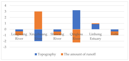
Figure 11.
The influence ratio of changes in environmental capacity of the estuaries of Haizhou Bay.
The difference between scenario B and estuary environmental capacity in 2006 reflects the impact of topographical changes on environmental capacity. The calculation results show that: the topographical changes caused by land reclamation reduced the environmental capacity of the coastal estuaries by a total of 14.021 tons/day from 2006. Specifically, the environmental capacity of Longwang River decreased by 17.678 tons/day, which accounted for 42% of the environmental capacity in 2006, and was 3.657 tons/day more than the total reduction in environmental capacity of all the coastal estuaries. The environmental capacity of Qingkou River increased by 4.362 tons/day, an increase of 45.84% from 2006. The environmental capacity of the remaining three estuaries slightly increased. It should be noted that the reduction in environmental capacity caused by land reclamation reached 42–46% because of the small environmental capacity of Xingzhuang River and Shawang River. The difference between scenario A and 2006 estuary environmental capacity reflects the impact of estuary runoff changes on the environmental capacity. The calculation results show that: the reduction in the aggregate discharge of runoff into the ocean decreased the environmental capacity by 22.97 tons/day, 8.952 tons/day more than that caused by land reclamation. This indicates that the impact of changes in runoff on the environmental capacity of the estuaries was 1.64 times that of land reclamation, which implies that the theoretical environmental capacity is more strongly influenced by the reduction in runoff than by land reclamation.
Moreover, increased runoff causes an increase in the environmental capacity of the estuaries, whereas a decrease in runoff reduces their environmental capacity. With the increase of the runoff, the velocity of the water into the sea increases, and the diffusion power is enhanced, so the environmental capacity increases. The reclamation project affects the current velocity and direction in the nearshore estuary area. If reclamation reduces the velocity of the estuary, the diffusion capacity decreases with the decrease of velocity, and the environmental capacity will decrease. Nevertheless, the impact of land reclamation on the environmental capacity of the estuary is fairly complex. It not only involves the land reclamation projects on both sides of the estuary, but also relates to the superimposed effects of multiple land reclamation projects in the estuary on the near-shore hydrodynamic environment. For example, there are large-scale reclamation projects on the north side of Qingkou River and the south side of Linhong Estuary, but the superimposed effects of these projects allowed these two estuaries to form a hydrodynamic pattern that facilitated water exchange with the waters outside the estuaries, thereby increasing the environmental capacity of the estuaries.
The resulting changes in environmental capacity of the coastal estuaries were consistent with the actual changes in 2016 and 2006 in both Path 1 and Path 2. This suggests that these two calculation paths can accurately simulate the simultaneous interactions and results of topography and runoff into the ocean, and can be used as the basis for analysis of different influencing factors. According to Path 1, the influence ratio of topography and runoff into the ocean on the reduction in total environmental capacity of the coastal estuaries was 0.429:0.571. According to Path 1, the influence ratio of topography and runoff into the ocean on the reduction in total environmental capacity of the coastal estuaries was 0.298:0.702. This demonstrates that Path 1 based on topographic changes will magnify the role of changes in land reclamation, whereas Path 1 based on changes in pollutant discharge into the ocean will magnify the role of changes in runoff. By taking into account the roles of these two factors, therefore, the average of Path 1and Path 2 was adopted. The corresponding influence ratio of topography and runoff into the ocean on the reduction in total environmental capacity of the coastal estuaries was 0.363:0.637. The runoff into the ocean therefore played a larger role in controlling the changes in environmental capacity at 1.75 times the impact of land reclamation on average.
The preceding analysis showed that land reclamation was not significantly positively or negatively correlated with the impact on coastal estuaries. Land reclamation primarily influences the structure of the tidal dynamic field through coastal land reclamation projects, hence influencing the diffusion and transport capabilities of the estuaries and changing the environmental capacity. The amount of runoff into the ocean is positively correlated with the impact on the environmental capacity of coastal estuaries. The vast differences in the amount of runoff and in the changes in runoff of different estuaries, as well as the impact of land reclamation projects, lead to major uncertainties in the changes in the environmental capacity of the coastal estuaries. The changes in hydrological characteristics and environmental capacity of the estuaries from 2006 to 2016 (Table 9) shows that the impact on environmental capacity of the estuaries is not only associated with the amount of runoff or the absolute value of changes in runoff, but also affected by the relative value of such changes, especially in the estuaries with large runoff. This is strongly related to the impact of changes in relative value. The considerable decrease in runoff of estuaries with large runoff, however, will inevitably drastically reduce the environmental capacity of the estuaries. Overall, the changes in the environmental capacity were decided by the interactions of the amount of runoff, the extent of changes in runoff, and the changes in hydrodynamics affected by land reclamation.
Table 9.
The changes in conditions and environmental capacity in the coastal estuaries of Haizhou Bay from 2006 to 2016.
The changes in and the corresponding relationships of the actual COD discharge, theoretical environmental capacity, and remaining environmental capacity of the estuaries of Haizhou Bay from 2006 to 2016 are complex. The estuaries with large actual discharge are decisive in controlling the theoretical environmental capacity of the coastal estuaries. Therefore, such estuaries should not only be the focus of the study on the environmental capacity of the coastal estuaries, but also the key areas for enacting controls on land-based pollutant release. In general, the reduction in runoff into the ocean will decrease the theoretical environmental capacity, but the actual discharge is also affected by the concentration of pollutants discharged into the ocean. The actual discharge is therefore not clearly positively or negatively correlated with the changes in environmental capacity. Moreover, the remaining environmental capacity is not associated with the theoretical one. Intriguingly, the reduction in runoff into the ocean will reduce the environmental capacity of the estuaries, but it will also decrease the aggregate discharge of pollutants, so the remaining environmental capacity may increase.
5. Conclusions
- (1)
- The actual aggregate discharge of the five coastal estuaries in Haizhou Bay was 102.352 tons/day in 2006, and 76.589 tons/day in 2016, reducing by 25.763 tons/day (25.17%). The theoretical environmental capacity was 114.571 tons/day in 2006, and 81.853 tons/day in 2016, reducing by 32.718 tons/day (28.56%). The remaining environmental capacity was 12.219 tons/day in 2006, and 5.264 tons/day in 2016, reducing by 6.955 tons/day (56.92%).
- (2)
- The changes in topography and pollutant discharge into the ocean in the estuaries of Haizhou Bay between 2006 and 2016 reduced the total environmental capacity of the estuaries with an influence ratio of 0.363:0.637. Moreover, the pollutant discharge into the ocean strongly impacted the changes in environmental capacity (1.75 times the impact of land reclamation on average). Land reclamation was not significantly positively or negatively correlated with the impact on coastal estuaries. Land reclamation primarily influenced the structure of the tidal dynamic field through coastal land reclamation projects, hence influencing the capability of hydrodynamics to diffuse and transport and changing the environmental capacity. Runoff into the ocean was positively correlated with the impact on the environmental capacity of coastal estuaries. However, the vast differences in the amount of runoff and in the changes in runoff of different estuaries, as well as the impact of land reclamation projects cause the changes in the environmental capacity of the coastal estuaries to be highly uncertain.
- (3)
- The changes in and the corresponding relationships of the actual COD discharge, theoretical environmental capacity, and remaining environmental capacity of the estuaries of Haizhou Bay from 2006 to 2016 are complex. Estuaries with large actual discharge play a decisive role in the theoretical environmental capacity, so these areas are key for control of aggregate land-based pollutant release into the ocean. The reduction in runoff into the ocean will decrease the theoretical environmental capacity. The remaining environmental capacity is not associated with the theoretical value and the reduction in runoff into the ocean will sometimes reduce the decrease the aggregate discharge of pollutants and increase the remaining environmental capacity.
Author Contributions
L.S. carried out the numerical simulation. L.S. and J.W. cartography and analyzed the data; H.Z. provided support to model setup and validation; L.S., J.W., H.Z., and M.X. discussed the result; original draft was written by L.S. and J.W.; All authors have read and agreed to the published version of the manuscript.
Funding
This research was funded by “Jiangsu Provincial Marine Science and Technology Innovation Project, grant number HY2018-3”.
Conflicts of Interest
The authors declare no conflict of interest.
References
- O’Driscoll, M.; Clinton, S.; Jefferson, A.; Manda, A.; McMillan, S. Urbanization Effects on Watershed Hydrology and In-Stream Processes in the Southern United States. Water 2010, 2, 605–648. [Google Scholar] [CrossRef]
- Pérez, P.; Fernández, E.; Beiras, R. Fuel toxicity on Isochrysis galbana and a coastal phytoplankton assemblage: Growth rate vs. variable fluorescence. Ecotoxicol. Environ. Saf. 2010, 73, 254–261. [Google Scholar] [CrossRef]
- Yu, C.Y.; Liang, B.; Han, G.C.; Huo, C.L.; Zhang, Z.F.; Ma, M.H. Discussion on the procedure and method of Marine oil spill ecological damage assessment. Ocean Dev. Manag. 2015, 32, 92–96. [Google Scholar] [CrossRef]
- Muller, J.R.M.; Chan, Y.-C.; Piersma, T.; Chen, Y.-P.; Aarninkhof, S.G.J.; Hassell, C.J.; Tao, J.-F.; Gong, Z.; Wang, Z.B.; van Maren, D.S. Building for Nature: Preserving Threatened Bird Habitat in Port Design. Water 2020, 12, 2134. [Google Scholar] [CrossRef]
- Benjamins, S.; Masden, E.; Collu, M. Integrating Wind Turbines and Fish Farms: An Evaluation of Potential Risks to Marine and Coastal Bird Species. J. Mar. Sci. Eng. 2020, 8, 414. [Google Scholar] [CrossRef]
- Dong, Z.; Kuang, C.; Gu, J.; Zou, Q.; Zhang, J.; Liu, H.; Zhu, L. Total Maximum Allocated Load of Chemical Oxygen Demand Near Qinhuangdao in Bohai Sea: Model and Field Observations. Water 2020, 12, 1141. [Google Scholar] [CrossRef]
- Yang, J.W. Theory and Practice of Conducting Total-Quantity Control of Pollutants Discharge in the Near shore Sea Area. Mar. Inf. 2001, 2, 24–26. [Google Scholar] [CrossRef]
- Pravdić, V.; Juračić, M. The environmental capacity approach to the control of marine pollution: The case of copper in the Krka River Estuary. Chem. Ecol. 1988, 3, 105–117. [Google Scholar] [CrossRef]
- Krom, M.D.; Hornung, H.; Cohen, Y. Determination of the environmental capacity of Haifa Bay with respect to the input of mercury. Mar. Pollut. Bull. 1990, 21, 349–354. [Google Scholar] [CrossRef]
- Nam, J.; Chang, W.; Kang, D. Carrying capacity of an uninhabited island off the southwestern coast of Korea. Ecol. Model. 2010, 221, 2102–2107. [Google Scholar] [CrossRef]
- Pandolfi, J.M.; Bradbury, R.; Sala, E.; Hughes, D.P.M.; Bjorndal, K.A.; Cooke, R.G.; McArdle, D.; McClenachan, L.; Newman, M.J.H.; Paredes, G.; et al. Global trajectories of the longterm decline of coral reef ecosystems. Science 2003, 301, 955–958. [Google Scholar] [CrossRef] [PubMed]
- Trela, J.; Płaza, E. Innovative technologies in municipal wastewater treatment plants in Sweden to improve Baltic Sea water quality. Proc. E3S Web Conf. 2018, 45, 113. [Google Scholar] [CrossRef]
- Gu, J.; Li, Z.Y.; Mao, X.D.; Hu, C.F.; Kuang, C.P. Study of COD environmental capacity in coastal waters of Beidaihe in summer. Mar. Environ. Sci. 2017, 36, 682–687. [Google Scholar] [CrossRef]
- Yu, Y.; Peng, C.S.; Yu, L.L.; Gu, Q.B.; Chang, J.M. Environmental capacity calculation of petroleum hydrocarbons in Laizhou Bay—The discharge optimization method based on the nonlinear programming. Mar. Environ. Sci. 2014, 33, 293–299. [Google Scholar] [CrossRef]
- Lan, D.D.; Liang, B.; Ma, M.H.; Yu, C.Y.; Bao, C.G.; Xu, Y. Application of marine environmental capacity analysis in planning environmental impact assessment. Ocean Dev. Manag. 2013, 30, 62–65. [Google Scholar]
- Sun, X.M.; Zhang, C.Z.; Shen, X.W. Total amount control of pollutant discharged into sea area around Changxingdao Island. Mar. Environ. Sci. 2009, 28, 399–402. [Google Scholar]
- Zhang, X.Q.; Sun, Y.L. Study on the environmental capacity in Jiaozhou Bay. Mar. Environ. Sci. 2007, 26, 347–350. [Google Scholar]
- Yu, J.; Sun, Y.L.; Zhang, Y.M.; Zhang, Y.; Cai, H.W. Environmental capacity assessment of pollutants in Ningbo-Zhoushan sea area. Environ. Pollut. Control 2006, 28, 21–24. [Google Scholar]
- Guo, L.B.; Jiang, W.S.; Li, F.Q.; Wang, X.L. Environmental Capacity Calculation of COD and PHs in the Bohai Sea. Period. Ocean Univ. China 2007, 37, 310–316. [Google Scholar] [CrossRef]
- Long, Y.X.; Chen, J.; Han, B.X. Research on Marine Environmental Capacity in the Beibu Gulf Economic Zone. Acta Sci. Nat. Univ. Sunyatseni 2014, 53, 83–88. [Google Scholar] [CrossRef]
- Zhai, D.S.; Zhang, K.; Sun, H.Y. Study on the coastal marine water environmental capacity of the Yangpu Economic Development Zone. J. Henan Agric. Univ. 2014, 48, 348–353. [Google Scholar] [CrossRef]
- Shi, P.; Peng, K.L.; Xie, J.; He, G.F. Study on the selection of discharge outlet int the sea of pollutants from coastal industry: With example of Zhanjiang Steel project. Trans. Oceanol. Limnol. 2011, 2, 159–166. [Google Scholar] [CrossRef]
- Wang, C.Y.; Wang, X.L.; Li, K.Q.; Liang, S.K.; Sun, R.G.; Yang, S.P. The estimation of copper, lead, zinc and cadmium fluxes into the sea area of the East China Sea interferenced by terrigenous matter and their environmental capacities. Acta Oceanol. Sin. 2010, 32, 62–76. [Google Scholar] [CrossRef]
- Liu, S.M.; Ye, X.W.; Zhang, J. The silicon balance in Jiaozhou Bay, North China. J. Mar. Syst. 2008, 74, 639–648. [Google Scholar] [CrossRef]
- Cui, J.R.; Zhang, L.P. Determination and Application of Pollutant Transfer and Transformation Modelin the Study of Xiamen Bay Environmental Capacity. Environ. Sci. Manag. 2009, 34, 10–14. [Google Scholar]
- Pan, C.M.; Zhang, L.P.; Huang, J.L.; Cui, J.R. Estimation of marine pollution load in West Sea and Tong’an Bay in Xiamen. Mar. Environ. Sci. 2011, 30, 90–95. [Google Scholar]
- Ke, L.N.; Wang, Q.M.; Xu, L.W.; Jiang, X.; Yang, S.L. The coastwise surplus water environment capacity computing model based on GIS. Mar. Sci. 2015, 39, 112–117. [Google Scholar]
- Wang, W.P. Study on Simulation of the Water Environmental Capacity Change and Controlling Measures of the Total Amount Pollutants Discharge in Jiulong River Watershed. Ph.D. Thesis, Xiamen University, Xiamen, China, 2007. [Google Scholar]
- Ge, S.F. Study on Water Environmental Capacity of Liaohe River in Jilin Province. Ph.D. Thesis, Jilin University, Changchun, China, 2012. [Google Scholar]
- Ou, M.L. Study on Impact of Three Gorges Reservoir Operation on Variation Characteristics of Nitrogen and Phosphorus in Waters of Poyang Lake. Master’s Thesis, East China University of Technology, Nanchang, China, 2012. [Google Scholar]
- Ma, X.X.; Li, C.Y.; Shi, X.H.; Zhao, S.N.; Sun, B.; Zhu, Y.H. Environment Capacity of the Wuliangsuhai Lake. J. Irrig. Drain. 2019, 38, 105–112. [Google Scholar] [CrossRef]
- Tang, J.Y. Research of Volume Control and Emission Reduction of COD, Nitrogen, Phosphorus in Water of Pulandian Bay. Master’s Thesis, Dalian Maritime University, Dalian, China, 2016. [Google Scholar]
- Jiang, H.Z.; Cui, L.; Yu, D.T.; Gao, F.; Wu, L.G. Study on sea area Environmental capacity of Majiazui sewage Outlet on Changxing Island in Dalian. J. Appl. Oceanogr. 2017, 36, 202–209. [Google Scholar] [CrossRef]
- Chen, Y. Environmental Capacity and Total Quantity Control of Nitrogen and Phosphorus in the Northern Part of Liaodong Bay. Master’s Thesis, Shanghai Ocean University, Shanghai, China, 2017. [Google Scholar]
- Lin, L.; Liu, D.Y.; Liu, Z.; Gao, H.W. Impact of land reclamation on marine hydrodynamic and ecological environment. Haiyang Xuebao 2016, 38, 1–11. [Google Scholar] [CrossRef]
- Wang, X. Environmental Capacity Value Loss Evaluation Research of Coastal Reclamation Projects in Bay Based on the Numerical Simulation—Case Study of Shacheng Harbor in Fujian Province. Master’s Thesis, Xiamen University, Xiamen, China, 2014. [Google Scholar]
- Garcia, M.; Ramirez, I.; Verlaan, M.; Castillo, J. Application of a three-dimensional hydrodynamic model for San Quintin Bay, B.C., Mexico. Validation and calibration using OpenDA. J. Comput. Appl. Math. 2015, 273, 428–437. [Google Scholar] [CrossRef]
- Dai, P.; Zhang, J.-s.; Zheng, J.-h.; Hulsbergen, K.; van Banning, G.; Adema, J.; Tang, Z.-x. Numerical study of hydrodynamic mechanism of dynamic tidal power. Water Sci. Eng. 2018, 11, 220–228. [Google Scholar] [CrossRef]
- Putzu, S.; Enrile, F.; Besio, G.; Cucco, A.; Cutroneo, L.; Capello, M.; Stocchino, A. A Reasoned Comparison between Two Hydrodynamic Models: Delft3D-Flow and ROMS (Regional Oceanic Modelling System). J. Mar. Sci. Eng. 2019, 7, 464. [Google Scholar] [CrossRef]
- Rueda-Bayona, J.G.; Osorio, A.F.; Guzman, A. Set-up and input dataset files of the Delft3d model for hydrodynamic modelling considering wind, waves, tides and currents through multidomain grids. Data Brief 2020, 28, 104921. [Google Scholar] [CrossRef] [PubMed]
Publisher’s Note: MDPI stays neutral with regard to jurisdictional claims in published maps and institutional affiliations. |
© 2020 by the authors. Licensee MDPI, Basel, Switzerland. This article is an open access article distributed under the terms and conditions of the Creative Commons Attribution (CC BY) license (http://creativecommons.org/licenses/by/4.0/).