Research into the Automatic Berthing of Underactuated Unmanned Ships under Wind Loads Based on Experiment and Numerical Analysis

Abstract

With the continuous improvement of unmanned ship automation requirements, research into the automatic berthing of underactuated unmanned ships has important theoretical significance and practical value. In order to determine the trajectory of unmanned ships, the line of sight (LOS) algorithm was applied due to the characteristics of underactuated unmanned ships without side thrusters. In order to resist wind disturbance, the active disturbance rejection control (ADRC) method was applied to keep the ship moving on its intended trajectory. Then, to carry out the simulation analysis before the tank experiment, a remote-control simulation system based on a user datagram protocol (UDP) communication was built, and the ability of the ADRC controller to make the ship perform completely automatic berthing in both wind and no wind conditions was verified in simulations. Combined with the simulation results, a tank experiment was accomplished at the Japanese National Research Institute of Fishery Engineering. The experimental results also showed that the ADRC controller has good robustness, that the problems of insufficient autonomous route determination and the disturbance rejection ability in the process of the automatic berthing of underactuated unmanned ships are solved, and the safety of ship navigation is improved, which lays a theoretical and experimental foundation for the further development of unmanned ship control.

1. Introduction

Although the current level of ship automation is relatively high and some small unmanned ship technology has become mature, it is seldom used in practice. The cargo throughput of the world’s major ports continues to rise. To improve transport efficiency, unmanned ships are a good choice in terms of safety, economy, and efficiency [1]. The world is competing to develop unmanned ship technology, with the United States and Israel leading in unmanned ship technology research [2,3,4,5]. MIT (The Massachusetts Institute of Technology) developed the Artemis unmanned ship in 1993, which can be used to test guidance, control, and propulsion systems. The unmanned ship was used to collect hydrological data from the Charles River in Boston. In 2000, MIT developed an AutoCat unmanned ship capable of remote control or autonomous navigation for survey missions. Israel has also made a tremendous contribution to the development of unmanned ships, especially regarding applications in the military. In 2003, the Rafal Corporation of Israel cooperated with the Israel Aviation Defense Systems Corporation to develop the famous unmanned ship Protector, which can be used for military tasks such as fire cover, antiterrorism, reconnaissance, antisubmarine, and electronic warfare. In 2016, Israel’s Elbit Systems Corporation developed the unmanned ship Silver Marlin, which is used for coastal intelligent patrol missions. Next, Israel developed the unmanned ships Stingray and Starfish, increasing the strength of its modern navy.

Research into the automatic berthing of underactuated ships is theoretically classified as the feedback stabilization control of underactuated systems. Trajectory design is needed in automatic berthing control. Ahmed et al. enabled a ship to navigate along an imaged route and stop at a given place 1.5 times the ship’s length from the berth, which means they can complete the automatic berthing control task [6,7]. A value of 1.5 times the ship’s length is set to allow sufficient maneuvering space to cope with any adverse situation, so berthing maneuvering does not necessarily bring the ship close to the berth but can also stop the ship at a certain distance outside the berth. There is also a direct approach to the berthing mode. Park and others used the propellers of a twin-propeller twin-rudder ship and the front side thrusters to complete parallel berthing [8]. Tamara et al. in Japan completed the task of first stabilizing the ship out of the berth and then approaching the berth in parallel by using the front and rear side thrusters [9]. For underactuated ships, most of the above research results are difficult to adapt because of the lack of side thrusters. Therefore, the out-of-berth stabilization has more research value in the automatic berthing of underactuated ships. Kim et al. proposed a logic-based control method to drive the ship forward and backward repeatedly along the predetermined course and gradually approach the predetermined state [10]. In theory, this overcomes the limitation of the continuous incentive conditions and allows the ship’s speed to be negative, but the drawbacks are obvious. Liu Yang et al. used the nonlinear adaptive control algorithm to design the trajectory tracking controller and berthing controller. The nonholonomic system was transformed into a cascade nonlinear system, and then the adaptive neural network algorithm was used to solve the uncertainty of disturbance. The stability of the closed-loop system was analyzed using the Lyapunov theory [11].

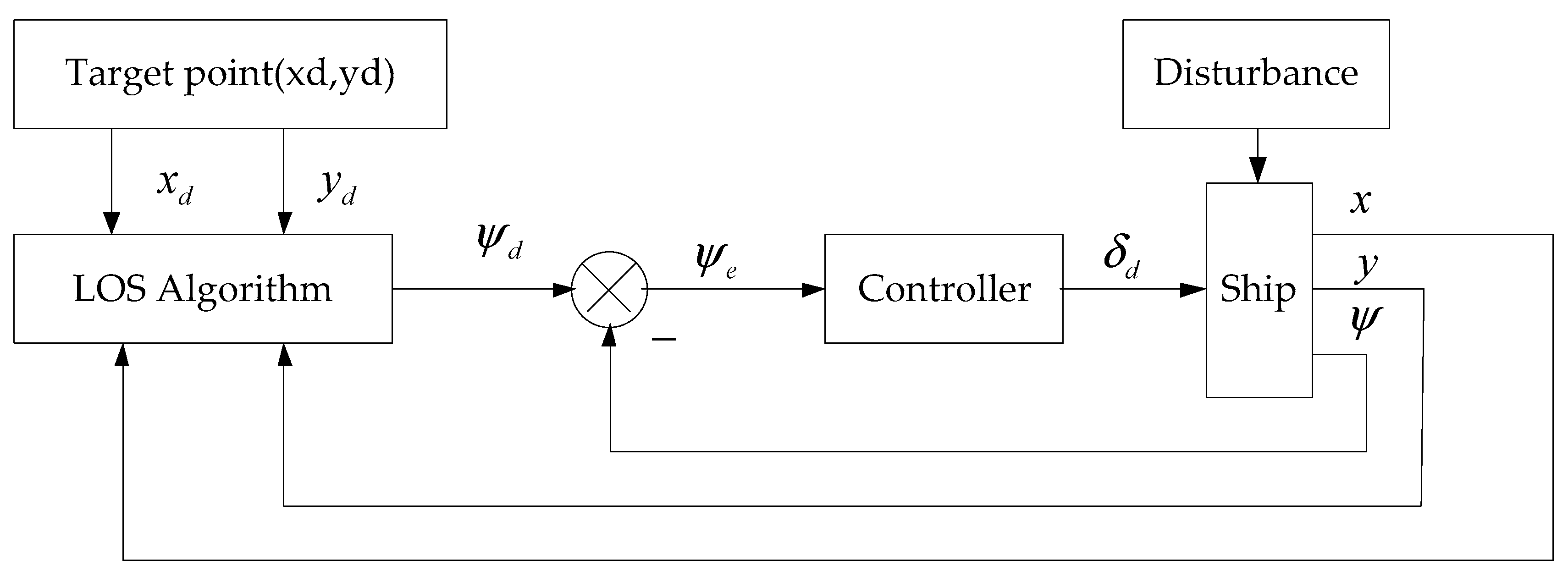
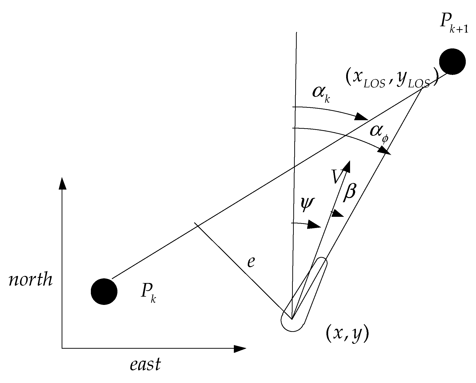
The rest of this paper is organized as follows: Section 2 introduces the automatic berthing mode using the line of sight (LOS) algorithm. The mathematical models of ship motion and wind are also established. Section 3 introduces the design of the controller and the method of parameter tuning. Section 4 carries out the simulation analysis of an unmanned ship and establishes a remote real-time control platform based on user datagram protocol (UDP) communication. Section 5 shows the results of an automatic berthing experiment for unmanned ships at the Japanese National Research Institute of Fishery Engineering.

The main contributions of this article are summarized as follows:

(1)

A mathematical model of underactuated unmanned ships and wind force is established to enhance berthing simulation, and an automatic berthing route determination method based on the LOS algorithm is proposed, with the control states set as the rudder angle and RPM (revolutions per minute), which meets the actual engineering requirements better.

(2)

The parameter tuning methods of a proportional-integral-derivative controller (PID) and active disturbance rejection control (ADRC) in the automatic berthing process are given. The tuning method of PID parameters adopts a closed-loop gain shaping algorithm, and ADRC adopts an innovative method based on the ship maneuverability index.

(3)

A remote real-time control platform based on UDP communication is established. It is a good alternative to the experiment tank system for the Japanese National Research Institute of Fishery Engineering.

(4)

An automatic berthing experiment for underactuated unmanned ships is carried out at the Japanese National Research Institute of Fishery Engineering. It is concluded that the ADRC controller can achieve automatic berthing in windy conditions, and the result is better than that of the PID controller. The experiment proves that we have created a new, realizable, strategy for automatic berthing that improves the autonomous navigation ability of unmanned ships.

2. Problem Formulation

2.1. Automatic Berthing Mode Based on LOS Algorithm

Ship berthing is one of the most complex and difficult ship maneuvering motions. In practice, the berthing of a ship is affected by shallow water, low speed, the shore wall effect, and so on. The berthing often relies on tugboat assistant operation, but it can also be operated by self-reliance when conditions permit. Therefore, research on the automatic berthing control of underactuated ship has important practical significance.

The main difficulties in the design of automatic berthing control for underactuated ship lie in the following aspects: There is no lateral pushing device, but there is lateral drift motion; the maneuverability and rudder efficiency of ships are poor when moving at low speed; the problem of motion trajectory should be taken into account in stabilization control; the inertia of ships is relatively large, and the accuracy of speed and position of ships is demanded at the same time. In this paper, the method to stabilize berthing outside berth proposed by Hasegawa [12], a Japanese scholar, was adopted. The purpose of berthing is that the ship stops at a place, twice the length of the ship from the designated point, and the speed is less than 1 knot. The process of automatic berthing is shown in Figure 1.

The problem of automatic berthing can be simplified as following a fixed trajectory to a specified position after a ship has reached a certain position, which is essentially a ship trajectory tracking problem. The ship trajectory tracking problem belongs to the dynamic positioning problem in a broad sense. The control schematic diagram is shown in Figure 2.

The navigation principle of the LOS algorithm is embodied in its intuitive understanding between rudder steering and ship motion [13,14,15,16,17]. The principle holds that if the course of the ship is kept at the line of sight angle, then after proper control, the desired position will be reached and track tracking will be achieved. Moreover, the LOS algorithm can reduce the traditional control states from three degrees of freedom (ship position (x, y) and course) to two degrees of freedom (course and speed), which is particularly important for the control of underactuated ships.

As shown in Figure 3, it was assumed that the current desired position of track tracking is $P_{k+1}={[x_{k+1},y_{k+1}]}^T$; the last expected position is $P_k={[x_k,y_k]}^T$; the current position of the ship is $P={[x,y]}^T$. Then, the LOS angle can be calculated by Equation (1) [18]:

$${\psi }_{LOS}=\arctan (\raisebox{1ex}{$y_{k+1}-y$}\!\left/ \!\raisebox{-1ex}{$x_{k+1}-x$}\right.),\hspace{0.17em}\hspace{0.17em}\hspace{0.17em}\hspace{0.17em}\hspace{0.17em}{\psi }_{LOS}\in (-\pi ,\pi )\hspace{0.17em}\hspace{0.17em}.$$

(1)

When the LOS algorithm is applied to ship trajectory tracking, Figure 4 shows that the expected heading point $P_{LOS}={[x_{LOS},y_{LOS}]}^T$ is $\Delta =nL$ away from the projection point of the current position of the ship on the desired track. L is the length of the ship, and $\hspace{0.17em}\Delta$ is the visual distance of the ship. At this time, the LOS control algorithm can be written as Equation (2):

$$\hspace{0.17em}{\alpha }_{\varphi }={\alpha }_k+\arctan (\raisebox{1ex}{$-e$}\!\left/ \!\raisebox{-1ex}{$\Delta $}\right.),$$

(2)

where e represents the lateral tracking error of the controlled ship, and ${\alpha }_k$ represents the angle between the northward direction of the geodetic coordinate system and the desired track. This paper assumes that the heading angle deviation ${\psi }_e={\alpha }_{\varphi }-\psi$, and when ${\psi }_e$ tends to zero, the self-propelled model travels to the target heading point and finally reaches the desired track to complete the trajectory tracking.

Suppose that there is a circle with the center of the current heading-looking point $(x_{k+1},y_{k+1})$, and the radius is R. At a certain moment, the current position $(x_k,y_k)$ of the controlled ship satisfies the following Equation (3):

$${(x_{k+1}-x_k)}^2+{(y_{k+1}-y_k)}^2\le R^2.$$

(3)

2.2. Mathematical Model of Unmanned Ship

There are two kinds of mathematical models of ship motion, separated and integral. At the end of the 1970s, the Japanese ship maneuvering mathematical model group (MMG) proposed a set of ship motion mathematical models, often referred to as the MMG model. Its main feature is the role of ship hydrodynamic forces and moments according to the physical significance, decomposing hydrodynamic forces and moments in the bare hull, propeller, rudder, and interference with each other. The MMG equation with wind force and the moment of the unmanned ship is Equation (4) [19]:

$$\hspace{0.17em}\{\begin{array}{l}(m+m_x)\dot{u}-(m+m_y)vr=X_H+X_P+X_R+X_{wind}\\ (m+m_y)\dot{v}+(m+m_x)ur=Y_H+Y_P+Y_R+Y_{wind}\\ (I_{zz}+J_{zz})\dot{r}=N_H+N_P+N_R+N_{wind}\\ \dot{\psi }=r\\ {\dot{x}}_0=u\cos \psi -v\sin \psi \\ {\dot{y}}_0=v\cos \psi +u\sin \psi \end{array}$$

(4)

In Equation (4), m is the mass of ship hull; $m_x$ and $m_y$ are longitudinal and transverse added mass, respectively; $I_{zz}$ and $J_{zz}$ are the moment of inertia and additional moment of inertia; X, Y, and N represent vertical force, lateral force, and turning moment, respectively. The subscript H is hull viscous fluid force and moment; the subscript for P represents force and moment produced by the propeller; R represents force and moment produced by rudder; the wind represents disturbance of ocean wind; $x_0$ and $y_0$ are for the longitudinal and transverse position of the ship; v is the lateral velocity of the ship; u is the longitudinal velocity of the ship; Ψ is the heading angle; and r is the turning angular velocity.

The integral model considers the separation mechanism of the hull as a whole, and the influence between the various mechanisms has been taken into account by default in the test. After the relevant parameters of the ship are known, the definitions for $V,L,x_c$ are speed, ship length, and the coordinates of the center of gravity. Dimensionless quantities are in Equation (5) [20]:

$$\{\begin{array}{l}m\prime =m/(\frac{1}{2}\rho L^3),m=\rho \nabla \\ x_c{}^{\prime }=x_c/L\\ v^{\prime }=v/V\\ r^{\prime }=rL/V\\ I_{ZZ}{}^{\prime }=I_{ZZ}/(\frac{1}{2}\rho L),I_{ZZ}=\frac{m{L}^2}{16}\end{array}$$

(5)

In the upper Equation (5), $\rho$ is the water density, and $\nabla$ is the displacement.

The hydrodynamic derivative is the most important part of the mathematical model of ship motion. Clarke collated a large number of ship model experimental data and obtained 10 regression equations of hydrodynamic derivatives by the main parameters of the ship, which can be written as Equation (6) [21]:

$$\{\begin{array}{l}{Y}_{\dot{v}}{}^{\prime }=-[1+0.16C_{b}B/T-5.1{(B/L)}^2]\cdot \pi {(T/L)}^2\\ Y_{\dot{r}}=-[0.67B/L-0.0033{(B/T)}^2]\cdot \pi {(T/L)}^2\\ N_{\dot{v}}^{\prime }=-[1.1B/L-0.041B/T]\cdot \pi {(T/L)}^2\\ N_{\dot{r}}^{\prime }=-[1/12+0.017C_{b}B/T-0.33B/L]\cdot \pi {(T/L)}^2\\ Y_v^{\prime }=-[1+0.40C_{b}B/T]\cdot \pi {(T/L)}^2\\ Y_r^{\prime }=-[-1/2+2.2B/L-0.080B/T]\cdot \pi {(T/L)}^2\\ N_v^{\prime }=-[1/2+2.4T/L]\cdot \pi {(T/L)}^2\\ N_r^{\prime }=-[1/4+0.039B/T-0.56B/L]\cdot \pi {(T/L)}^2\\ Y_{\delta }^{\prime }=3.0A_{\delta }/L^2\\ N_{\delta }^{\prime }=-(1/2)Y_{\delta }^{\prime }\end{array}$$

(6)

In the upper Equation (6), $B,T,C_b$, and $A_{\delta }$ are the breadth of the ship, draft, square coefficient, and rudder angle; ${\mathrm{Y}}_{\mathrm{v}}^{,},{\mathrm{Y}}_{\mathrm{r}}^{,},{\mathrm{N}}_{\mathrm{v}}^{,},{ \mathrm{and} \mathrm{N}}_{\mathrm{v}}^{,}$ are the hydrodynamic derivatives of the hull itself. According to practical experience, it is necessary to revise them according to Equation (7) [20]:

$$\{\begin{array}{l}\Delta Y^{\prime }v=-\gamma Y^{\prime }\delta \\ \Delta Y^{\prime }r=-1/2(\Delta Y^{\prime }v)\\ \Delta N^{\prime }v=-1/2(\Delta Y^{\prime }v)\\ \Delta N^{\prime }r=1/4(\Delta Y^{\prime }v)\\ \gamma =0.30\end{array}$$

(7)

Thus, ${Y^{\prime }}_v={Y^{\prime }}_v+\Delta {Y^{\prime }}_v$, ${Y^{\prime }}_r={Y^{\prime }}_r+\Delta {Y^{\prime }}_r$, ${N^{\prime }}_v={N^{\prime }}_v+\Delta {N^{\prime }}_v$, ${N^{\prime }}_r={N^{\prime }}_r+\Delta {N^{\prime }}_r$ allow the ship to be modeled as a standard, dimensionless state space equation, Equation (8) [22]:

$$\left[\begin{array}{l}{m}^{\prime }-{Y^{\prime }}_{\dot{v}}\hspace{0.17em}\hspace{0.17em}\hspace{0.17em}\hspace{0.17em}\hspace{0.17em}\hspace{0.17em}L(m^{\prime }{x^{\prime }}_C-{Y^{\prime }}_{\dot{r}})\\ m^{\prime }{x^{\prime }}_C-{N^{\prime }}_{\dot{v}}\hspace{0.17em}\hspace{0.17em}\hspace{0.17em}L({I^{\prime }}_{zz}-{N^{\prime }}_r)\end{array}\right]\hspace{0.17em}\left[\begin{array}{l}\dot{v}\\ \dot{r}\end{array}\right]=\left[\begin{array}{l}\frac{V}{L}{Y^{\prime }}_{\dot{v}\hspace{0.17em}\hspace{0.17em}\hspace{0.17em}\hspace{0.17em}}\hspace{0.17em}\hspace{0.17em}V({Y^{\prime }}_r-m^{\prime })\\ \frac{V}{L}{N^{\prime }}_{v\hspace{0.17em}\hspace{0.17em}\hspace{0.17em}\hspace{0.17em}}\hspace{0.17em}\hspace{0.17em}V({N^{\prime }}_r-m^{\prime }{x^{\prime }}_C)\end{array}\right]\left[\begin{array}{l}v\\ r\end{array}\right]+\left[\begin{array}{l}\frac{V^2}{L}{Y^{\prime }}_{\delta }\\ \frac{V^2}{L}{Y^{\prime }}_{\delta }\end{array}\right]\delta$$

(8)

Equation (8) can be simplified to Equation (9):

$${\dot{X}}_{(2)}=A_{(2)}{X}_{(2)}+B_{(2)}\delta , A_{(2)}=\left[\begin{array}{cc}{a}_{11}& a_{12}\\ a_{21}& a_{22}\end{array}\right], B_{(2)}=\left[\begin{array}{c}{b}_{11}\\ b_{21}\end{array}\right]$$

(9)

$$\{\begin{array}{l}{a}_{11}=[(I_z^{\prime }-N_{\dot{r}}^{\prime })Y_v^{\prime }-(m^{\prime }{x}_c^{\prime }-Y_{\dot{r}}^{\prime })N_v^{\prime }]V/S_1\\ a_{12}=[(I_z^{\prime }-N_{\dot{r}}^{\prime })(Y_r^{\prime }-m^{\prime })-(m^{\prime }{x}_c^{\prime }-Y_{\dot{r}}^{\prime })(N_r^{\prime }-m^{\prime }{x}_c^{\prime })]LV/S_1\\ a_{21}=[-(m^{\prime }{x}_c^{\prime }-N_{\dot{v}}^{\prime })Y_v^{\prime }+(m^{\prime }-Y_{\dot{v}}^{\prime })N_v^{\prime }]V/L/S_1\\ a_{22}=[-(m^{\prime }{x}_c^{\prime }-N_{\dot{v}}^{\prime })(Y_r^{\prime }-m^{\prime })+(m^{\prime }-Y_{\dot{v}}^{\prime })(N_r^{\prime }-m^{\prime }{x}_c^{\prime })]V/S_1\\ b_{11}=[(I_z^{\prime }-N_{\dot{r}}^{\prime })Y_{\delta }^{\prime }-(m^{\prime }{x}_c^{\prime }-Y_{\dot{r}}^{\prime })N_{\delta }^{\prime }]V^2/S_1\\ b_{21}=[-(m^{\prime }{x}_c^{\prime }-N_{\dot{v}}^{\prime })Y_{\delta }^{\prime }+(m^{\prime }-Y_{\dot{v}}^{\prime })N_{\delta }^{\prime }]V^2/L/S_1\\ S_1=[(I_z^{\prime }-N_{\dot{r}}^{\prime })(m^{\prime }-Y_{\dot{v}}^{\prime })-(m^{\prime }{x}_c^{\prime }-N_{\dot{v}}^{\prime })(m^{\prime }{x}_c^{\prime }-Y_{\dot{r}}^{\prime })]L\end{array}$$

(10)

The integral model is:

$$G_{\psi \delta }(s)=\frac{K}{s(Ts+1)}.$$

(11)

Among it, $K=\frac{b_{11}{a}_{21}-b_{21}{a}_{11}}{a_{11}{a}_{22}-a_{12}{a}_{21}}$,$T=-(\frac{a_{11}+a_{22}}{a_{11}{a}_{22}-a_{12}{a}_{21}}+\frac{b_{21}}{b_{11}{a}_{21}-b_{21}{a}_{11}})$.

The wind force and moment can be calculated by Equation (12) [23]:

$$\{\begin{array}{l}{X}_{wind}=0.5{\rho }_a{U}_R{}^2{A}_f{C}_{wx}\\ Y_{wind}=0.5{\rho }_a{U}_R{}^2{A}_s{C}_{wy}\\ N_{wind}=0.5{\rho }_a{U}_R{}^2{A}_{s}L{C}_{wn}\end{array}$$

(12)

In Equation (12), ${\rho }_a$ is the air density; $U_R$ is the relative wind velocity; ${ A}_f$ is the orthogonal projection area of the hull surface; $A_s$ is the side of the projection area on the water line; and $C_{wx}$, $C_{wy}$, and $C_{wn}$ are the lateral and longitudinal direction of the wind pressure force coefficient and wind pressure moment coefficient, whose calculations are in Equation (13):

$$\{\begin{array}{l}{C}_{wx}=X_0+X_1\cos {\psi }_a+X_3\cos 3{\psi }_a+X_5\cos 5{\psi }_a\\ C_{wy}=Y_1\sin {\psi }_a+Y_3\sin 3{\psi }_a+Y_5\sin 5{\psi }_a\\ C_{wn}=N_1\sin {\psi }_a+N_2\sin 2{\psi }_a+N_3\sin 3{\psi }_a\end{array}$$

(13)

In Equation (13), ${\psi }_a$ is the attack angle. The serial numbers of $X_i$, ${ Y}_i$, and $N_i$ range from 1 to 5. Fujiwara obtained the parameter threshold for the calculation result after several experiments. The parameter exceeding the threshold is: $X_0$, $X_1$, $X_3$, $X_5$, $Y_1$, $Y_3$, $Y_5$, $N_1$, $N_2$, and $N_3$, calculated as Equations (14)–(16). L is the length of the ship; B is the breadth of the ship; $A_T$ is the transverse projected area of the ship; $A_L$ is the lateral projected area of the ship; $A_{OD}$ is the lateral projected area of the superstructure; C is the distance from midship to the center of the lateral projected area; $C_{BR}$ is the distance from midship to the center of the lateral projected area of superstructure; $H_{BR}$ is the height to the top of the superstructure; $H_C$ is the height to the lateral projected area; $x_{nm}$, $y_{nm}$, and $n_{nm}$ are a recursive coefficient obtained by the experiment and can be determined based on

Table 1. Each coefficient of independent variables.

m=	0	1	2	3	4	5	6	7	8
$x_{0m}$	−0.330	0.293	0.0193	0.682
$x_{1m}$	−1.353	1.700	2.87	−0.463	−0.570	−6.640	−0.0123	0.0202
$x_{3m}$	0.830	−0.413	−0.0827	−0.563	0.804	−5.67	0.0401	−0.132
$x_{5m}$	0.0372	−0.0075	−0.103	0.0921
$y_{1m}$	0.684	0.717	−3.22	0.0281	0.0661	0.298
$y_{3m}$	−0.400	0.282	0.307	0.0519	0.0526	−0.0814	0.0582
$y_{5m}$	0.122	−0.166	−0.0054	−0.0481	−0.0136	−0.0864	−0.0297
$n_{1m}$	0.299	1.71	0.183	−1.09	−0.0442	−0.289	4.24	−0.0646	0.0306
$n_{2m}$	0.117	0.123	−0.323	0.0041	−0.166	−0.0109	0.174	0.214	−1.06
$n_{3m}$	0.0230	0.0385	−0.0339	0.0023

.

$$\{\begin{array}{l}{X}_0=x_{00}+x_{01}\left(B{H}_{BR}\right)/A_T+x_{02}C/H_C+x_{03}{A}_{OD}/\left(L^2\right)\\ X_1=x_{10}+x_{11}{A}_L/\left(LB\right)+x_{12}L{H}_C/A_L+x_{13}L{H}_{BR}/A_L\\ \hspace{0.17em}\hspace{0.17em}\hspace{0.17em}\hspace{0.17em}\hspace{0.17em}+x_{14}{A}_{OD}/A_L+x_{15}{A}_T/\left(LB\right)+x_{16}{L}^2/A_T+x_{17}L/H_C\\ X_3=x_{30}+x_{31}{}_L/\left(L{H}_{BR}\right)+x_{32}{A}_L/A_T+x_{33}L{H}_C/A_L\\ \hspace{0.17em}\hspace{0.17em}\hspace{0.17em}\hspace{0.17em}\hspace{0.17em}+x_{34}{A}_{OD}/A_L+x_{35}{A}_{OD}/\left(L^2\right)+x_{36}C/H_C+x_{37}{C}_{BR}/L\\ X_5=x_{50}+x_{51}{A}_L/A_{OD}+x_{52}{C}_{BR}/L+x_{53}{A}_L/(LB)\end{array}$$

(14)

$$\{\begin{array}{l}{Y}_1=y_{10}+y_{11}{C}_{BR}/L+y_{12}C/L+y_{13}{A}_L/A_{OD}+y_{14}C/H_C+y_{15}{A}_T/\left(B{H}_{BR}\right)\\ Y_3=y_{30}+y_{31}{A}_L/\left(LB\right)+y_{32}L{H}_C/A_L+y_{33}{C}_{BR}/L+y_{34}B/H_{BR}+y_{35}{A}_{OD}/A_L+y_{36}{A}_T/\left(B{H}_{BR}\right)\\ Y_5=y_{50}+y_{51}{A}_L/\left(LB\right)+y_{52}L/H_{BR}+y_{53}{C}_{BR}/L+y_{54}B^2/A_T+y_{55}C/L+y_{56}L{H}_C/A_L\end{array}$$

(15)

$$\{\begin{array}{l}{N}_1=n_{10}+n_{11}C/L+n_{12}L{H}_C/A_L+n_{13}{A}_T/A_L+n_{14}C/H_C\\ \hspace{0.17em}\hspace{0.17em}\hspace{0.17em}\hspace{0.17em}\hspace{0.17em}+n_{15}{A}_L/\left(LB\right)+n_{16}{A}_T/\left(L^2\right)+n_{17}{B}^2/A_T+n_{18}{C}_{BR}/L\\ N_2=n_{20}+n_{21}{C}_{BR}/L+n_{22}C/L+n_{23}{A}_L/A_{OD}+n_{24}{A}_T/\left(B^2\right)\\ \hspace{0.17em}\hspace{0.17em}\hspace{0.17em}\hspace{0.17em}+n_{25}L/H_{BR}+n_{26}{A}_T/\left(B{H}_{BR}\right)+n_{27}{A}_L/\left(LB\right)+n_{28}{A}_L/\left(L^2\right)\\ N_3=n_{30}+n_{31}\ast C_{BR}/L+n_{32}\ast A_T/\left(B\ast H_{BR}\right)+n_{33}\ast A_L/A_T\end{array}$$

(16)

3. Controller Design and Parameter Tuning

In the experiment, the PID control algorithm and the ADRC algorithm were used. The two algorithms and their parameters’ respective tuning methods are introduced.

3.1. PID Algorithm

According to the closed-loop spectrum requirement of the system, this paper presents a method of PID parameter tuning based on closed-loop gain shaping. The solution process is simple, and the physical meaning is obvious. The designed PID controller has good robustness. The second-order object is Equation (17):

$$G=\frac{b_{1}s+b_0}{a_2{s}^2+a_{1}s+a_0}.$$

(17)

A practical engineering object can be transformed into a second-order object by model reduction or Bode graph approximation. According to the first-order closed-loop gain shaping algorithm, control $K_C$ can be calculated as Equation (18) [24]:

$$K_C=\frac{a_2{s}^2+a_{1}s+a_0}{b_0{T}_{01}s}=\frac{a_1}{b_0{T}_{01}}+\frac{a_0}{b_0{T}_{01}s}+\frac{a_{2}s}{b_0{T}_{01}}$$

(18)

In Equation (18), $T_{01}$ is time constant designed for the time based on the bandwidth frequency of the controlled object. It can be seen that Equation (18) is a standard PID controller, $k_p$, $k_i$, and $k_d$ are in Equation (19):

$$k_p=\frac{a_1}{b_0{T}_{01}},k_i=\frac{a_0}{b_0{T}_{01}},k_d=\frac{a_2}{b_0{T}_{01}}.$$

(19)

3.2. ADRC Algorithm

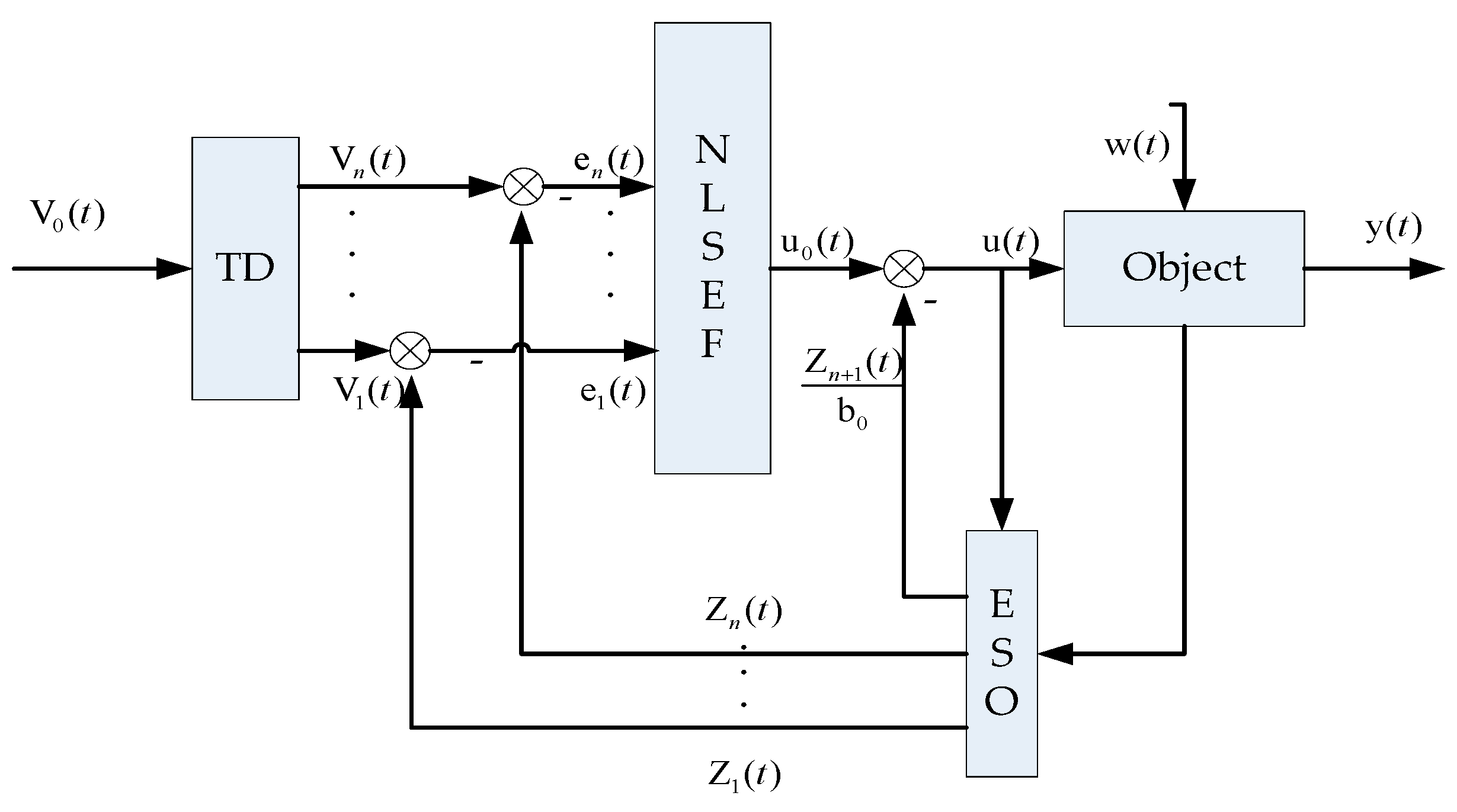
The active disturbance rejection control (ADRC) is not very strict with the mathematical model of the controlled object during disturbances, and it can, through the special structure of nonlinear feedback, compensate for the external and internal error of the system in time [25]. ADRC is mainly composed of a tracking differentiator (TD), extended state observer (ESO), and nonlinear state error feedback control law (NLSEF); the structure is shown in Figure 5.

Based on the second-order system as an example, this paper introduces the principle of ADRC, where the second-order controlled system state equation is Equation (20):

$$\{\begin{array}{l}{\dot{x}}_1=x_2\\ {\dot{x}}_2=f(x_1,x_2)+bu\\ y=x_1\end{array}.$$

(20)

In the second-order tracking differentiator, for example, differential Equation (21) is as follows:

$$\{\begin{array}{l}{\dot{x}}_1=x_2\\ {\dot{x}}_2=-fst(x_1,x_2,x,r,h_0)\end{array}.$$

(21)

Among them, v is the target signal; $v_1$ and $v_2$ are estimates of the target signal and its differential signal; $h_0$ is the filtering factor; r is the tracking speed factor; the expressions of nonlinear function $fst(v_1,v_2,v,r,h_0)$ are in Equation (22) [26]:

$$\{\begin{array}{l}d=r\cdot h\hspace{0.17em};\hspace{0.17em}{d}_0=d\cdot h;\hspace{0.17em}y=x_1-u+h\cdot x_2;\hspace{0.17em}\hspace{0.17em}{a}_0=\sqrt{d^2+8r\left|y\right|}\\ fst=\{\begin{array}{l}\frac{-r\cdot a}{d}\hspace{0.17em}\hspace{0.17em}\hspace{0.17em}\hspace{0.17em}\hspace{0.17em}\hspace{0.17em}\hspace{0.17em}\hspace{0.17em}\hspace{0.17em}\hspace{0.17em}\hspace{0.17em}\hspace{0.17em}\hspace{0.17em}\left|a\right|\le d\\ -r\cdot \mathrm{sgn}(a)\hspace{0.17em}\hspace{0.17em}\hspace{0.17em}\hspace{0.17em}\hspace{0.17em}\hspace{0.17em}\hspace{0.17em}\left|a\right|>d\end{array}\hspace{0.17em}\hspace{0.17em}\hspace{0.17em}a=\{\begin{array}{l}{x}_2+\frac{y}{h}\hspace{0.17em}\hspace{0.17em}\hspace{0.17em}\hspace{0.17em}\hspace{0.17em}\hspace{0.17em}\hspace{0.17em}\hspace{0.17em}\hspace{0.17em}\hspace{0.17em}\hspace{0.17em}\hspace{0.17em}\hspace{0.17em}\hspace{0.17em}\hspace{0.17em}\hspace{0.17em}\hspace{0.17em}\hspace{0.17em}\hspace{0.17em}\hspace{0.17em}\hspace{0.17em}\hspace{0.17em}\hspace{0.17em}\hspace{0.17em}\hspace{0.17em}\hspace{0.17em}\hspace{0.17em}\hspace{0.17em}\hspace{0.17em}\hspace{0.17em}\hspace{0.17em}\left|y\right|\le d_0\\ x_2+0.5(a_0-d)\cdot \mathrm{sgn}(y)\hspace{0.17em}\hspace{0.17em}\hspace{0.17em}\hspace{0.17em}\hspace{0.17em}\hspace{0.17em}\hspace{0.17em}\left|y\right|>d_0\end{array}\end{array}.$$

(22)

For the second-order system, expand the real-time action of the open-loop system acceleration $f(x_1(t),x_2(t))$ for the new state variables, and ${\dot{x}}_3=\phi (t)$ so that Equation (20) turns to Equation (23):

$$\{\begin{array}{l}{\dot{x}}_1=x_2\\ {\dot{x}}_2=f(x_1,x_2)+bu\\ {\dot{x}}_3=\phi (t)\\ y=x_1\end{array}$$

(23)

$e=z_1-y$, the nonlinear continuous observer of the system, is Equation (24):

$$\{\begin{array}{l}{\dot{z}}_1=z_2-{\beta }_{01}e\\ {\dot{z}}_2=z_3-{\beta }_{02}fal(e,a_{01},{\delta }_{01})+bu\\ {\dot{z}}_3=-{\beta }_{03}fal(e,a_{02},{\delta }_{02})\end{array}.$$

(24)

Among them, $z_1$ and $z_2$, respectively, represent the output of the object and its first-order differential; $z_3$ is for internal and external disturbance estimation; ${\beta }_{01}$, ${\beta }_{02}$, and ${\beta }_{03}$ are for the output error correction gain; the fal function is Equation (25) [26]:

$$fal(e,a,\delta )=\{\begin{array}{l}{\left|e\right|}^a\mathrm{sgn}(e),\left|e\right|>\delta \\ e/{\delta }^{1-a},\left|e\right|\le \delta \end{array}\delta >0.$$

(25)

Set $e_1=x_1-z_1;e_2=x_2-z_2$, and the nonlinear state error feedback control law is Equation (26):

$$u_0=k_{1}fal(e_1,a_1,{\delta }_1)+k_{2}fal(e_2,a_2,{\delta }_2).$$

(26)

${\beta }_1$, ${\beta }_2$, $a_1$, $a_2$, ${\delta }_1$, and ${\delta }_2$ are all adjustable parameters, while $e_1$ and $e_2$ represent the state error.

The basis calculation method of the ADRC parameters can be carried out as follows:

(1) For TD, r determines the tracking speed of the tracking signal. The smaller the tracking speed, the better it can suppress overshoot. If r is too small, it will affect the response speed of the system. For h, when the simulation step size is determined, the steady-state flutter can be eliminated as long as h is larger than the simulation step.

(2) ESO stability is the main objective of parameter adjustment, generally taking $a_{01}=0.5$, $a_{02}=0.25$, ${\beta }_{01}h=1$, ${\beta }_{02}=\frac{{\beta }_{01}}{h}$, and ${\beta }_{03}=\frac{{\beta }_{02}}{h}$.

(3) The two parameters of NLSEF have relatively clear meanings. Compared with PID, $k_1$ is equivalent to the proportional coefficient, $k_2$ almost equivalent to the differential coefficient, and its function is similar to that of PID.

(4) The function of parameter b is to produce a large error control signal when the system has a delay, and the corresponding system response becomes slower. It is similar to the integral coefficient. A system with a b value that is too small may be unstable, and a b value that is too large will slow down the response of the system.

In the specific application process, the discussed methods need to be debugged many times, because the control parameters of ADRC do not depend on the mathematical model, and the actual nonlinear factors on the effect of the controller need to be avoided. Next, a more general method for calculating parameters is proposed. In summary, the controller equations of ADRC are in Equation (27):

$$\hspace{0.17em}\{\begin{array}{l}e=z_1-y\\ {\dot{z}}_1=z_2-{\beta }_{01}e\\ {\dot{z}}_2=z_3-{\beta }_{02}fal(e,a_{01},{\delta }_{01})+bu\\ {\dot{z}}_3=-{\beta }_{03}fal(e,a_{02},{\delta }_{02})\\ e_1=x_1-z_1;e_2=x_2-z_2\\ u_0=k_{1}fal(e_1,a_1,{\delta }_1)+k_{2}fal(e_2,a_2,{\delta }_2)\\ u=u_0-z_3/b\end{array}.$$

(27)

The parameters that need to be tuned are the following: $ESO:b_{},{\beta }_{01},{\beta }_{02},{\beta }_{03};\hspace{0.17em}NLSEF:k_1,k_2$. The rest of the parameters can be taken as follows: TD: r = 100; h = 2, $ESO:a_{01}=0.5$, $a_{02}=0.25$, ${\delta }_{01}={\delta }_{02}=0.1$; $NLSEF$$:a_1=0.75$, $a_2=2.75$, ${\delta }_1={\delta }_2=0.1$.

According to gain K of the ship integral model, it can be assumed that: $p=1/\sqrt{K}$; next, a second-order controlled system is taken as an example to study the ADRC parameter tuning method based on manipulability index p.

There is a standard system Equation (28):

$$S1:\{\begin{array}{l}{\dot{x}}_{11}=x_{12}\\ {\dot{x}}_{12}=f_1(x_{11},x_{12},t_1)+b_1^{\ast }{u}_1\\ y_1=x_{11}\end{array}ADR{C}_1:\hspace{0.17em}\hspace{0.17em}\{\begin{array}{l}{e}_{01}=z_{11}-y_1\\ {\dot{z}}_{11}=z_{12}-{\beta }_{11}{e}_{01}\\ {\dot{z}}_{12}=z_{13}-{\beta }_{12}fal(e_{01},a_{01},{\delta }_{01})+b_1{u}_1\\ {\dot{z}}_{13}=-{\beta }_{13}fal(e_{01},a_{02},{\delta }_{02})\\ e_{11}=x_{11}-z_{11};e_{12}=x_{12}-z_{12}\\ u_{01}=k_{11}fal(e_{11},a_1,{\delta }_1)\\ \hspace{0.17em}\hspace{0.17em}\hspace{0.17em}\hspace{0.17em}\hspace{0.17em}\hspace{0.17em}+k_{12}fal(e_{12},a_2,{\delta }_2)\\ u_1=u_{01}-z_{13}/b_1\end{array}.$$

(28)

The manipulability index of S1 is $p_1$, and the parameters of the controller have been set. Now the following system parameters need to be tuned in Equation (29):

$$S2:\{\begin{array}{l}{\dot{x}}_{21}=x_{22}\\ {\dot{x}}_{22}=f_2(x_{21},x_{22},t_2)+b_2^{\ast }{u}_2\\ y_2=x_{21}\end{array}ADR{C}_2:\{\begin{array}{l}{e}_{02}=z_{21}-y_2\\ {\dot{z}}_{21}=z_{22}-{\beta }_{21}{e}_{02}\\ {\dot{z}}_{22}=z_{23}-{\beta }_{22}fal(e_{02},a_{01},{\delta }_{01})+b_2{u}_2\\ {\dot{z}}_{23}=-{\beta }_{23}fal(e_{02},a_{02},{\delta }_{02})\\ e_{21}=x_{21}-z_{21};e_{22}=x_{22}-z_{22}\\ u_{02}=k_{21}fal(e_{21},a_1,{\delta }_1)\\ \hspace{0.17em}\hspace{0.17em}\hspace{0.17em}\hspace{0.17em}\hspace{0.17em}+k_{22}fal(e_{22},a_2,{\delta }_2)\\ u_2=u_{02}-z_{23}/b_2\end{array}.$$

(29)

The manipulability index of S2 is $p_2$, $m=\raisebox{1ex}{$p_1$}\!\left/ \!\raisebox{-1ex}{$p_2$}\right.$, according to the concept of time scale proposed by Professor Han, and Equation (27) is changed to Equation (30):

$$\{\begin{array}{l}{e}_{01}=z_{11}-y_1\\ {\dot{z}}_{11}=z_{12}-{\beta }_{21}{e}_{01}/m\\ {\dot{z}}_{12}=z_{13}-{\beta }_{22}fal(e_{01},a_{01},{\delta }_{01})/m^2+b_2{u}_2/m^2\\ {\dot{z}}_{13}=-{\beta }_{23}fal(e_{01},a_{02},{\delta }_{02})/m^3\\ e_{21}=x_{11}-z_{11};e_{12}=x_{12}-z_{12}\\ u_{02}=k_{21}fal(e_{11},a_1,{\delta }_1)+k_{22}mfal(e_{12},a_2,{\delta }_2)\\ u_2=u_{02}-z_{13}/(b_2/m^2)\end{array}.$$

(30)

Then the parameter setting equations are obtained in Equation (31):

$${\beta }_{21}=m{\beta }_{11},{\beta }_{22}=m^2{\beta }_{12},{\beta }_{23}=m^3{\beta }_{13},k_{21}=k_{11},k_{22}=1/m{k}_{12},b_2=m^2{b}_1.$$

(31)

4. Automatic Berthing Simulation

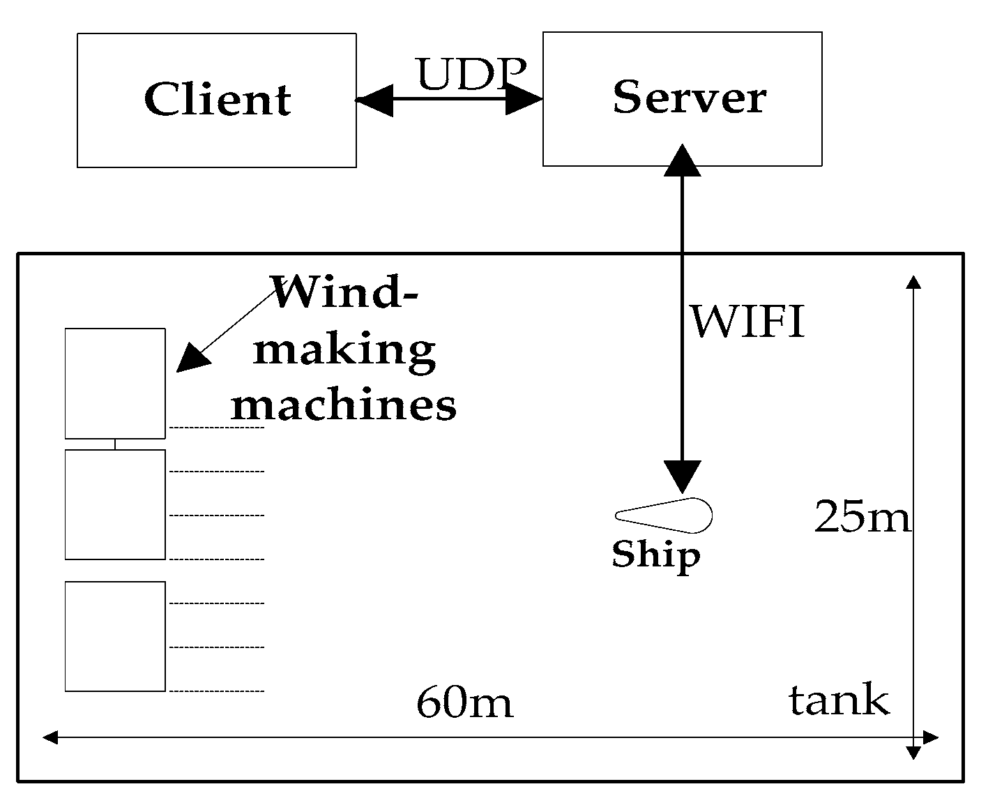
The tank experiment was carried out at the Japan National Research Institute of Fisheries Engineering, so the simulation is aimed at this experiment. The experiment mode is shown in Figure 6. The client and the server communicate with each other through UDP, and the server communicates with the ship through Wi-Fi. Because the server is written in python, in the simulation, the server was also written in Python to publish and receive data, and the client was written in MATLAB/Simulink to achieve ship motion control.

An unmanned ship has a unique communication system. Because there is no personnel on board, it is very important to exchange information with the shore. Common communication protocols include the transmission control protocol/internet protocol (TCP/IP), UDP, serial communication protocol, wireless network protocol, etc. [27,28,29]. TCP is a reliable communication protocol, that is, before formal communication between the two sides, it is necessary to establish a connection to ensure that data are not lost. Therefore, the transmission speed of data is relatively slow, and UDP only needs to set a port and IP address to send data, which does not guarantee the reliability of data (i.e., the possibility of packet loss), so it is an unreliable communication protocol, but UDP has a transmission speed that TCP cannot match.

As a general control system simulation software, MATLAB has been widely used for its powerful functions. In the research of control theory, the design and simulation of control law can be conveniently carried out using MATLAB/Simulink. In simulation tests, it is often necessary to connect external hardware simulation equipment for real-time simulation research. However, in the past, MATLAB/Simulink lacked the ability of real-time simulation. Usually, we need to write another application program that can simulate real time to do this work. In this way, the function of real-time simulation software is relatively singular, involving substantial repetitive work, and debugging is difficult. In addition, the communication between MATLAB and other platforms has not been studied much, which is not conducive to the direct application of MATLAB for actual control. Therefore, it is necessary to explore how to carry out real-time control in MATLAB/Simulink. Using the interface of MATLAB/Simulink and an external program to exchange data with the external control program through shared memory, real-time communication across platforms, and real-time simulation of ship motion control with high accuracy can be realized.

A 7.2-scale fishing ship named Kosoko was used in the experiment. The dimensions of the ship are shown in

Table 2. Ship dimensions.

Description	Ship Scale	Model Scale
Length	12.00 m	1.667 m
Breadth	5.10 m	0.701 m
Draft	1.00 m	0.138 m

.

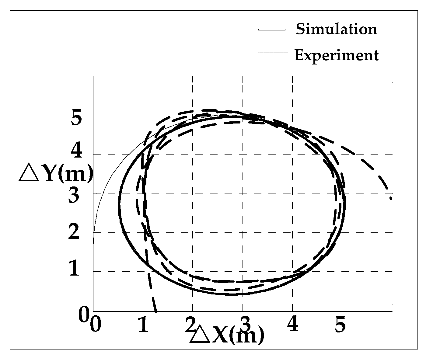
Firstly, a ship maneuverability simulation was carried out to verify the accuracy of the ship mathematical model. The turning experiment and zig-zag experiment are the two most important experiments to test ship maneuverability [30,31]. The simulation results of the +35 deg turning test are shown in Figure 7.

In Figure 7, △X and △Y is the change of position. Set the current position to (x,y) and the initial position to ($x_{0,}{y}_0$), so △X = x − $x_0$, △Y = x − $y_0$; the simulation data are analyzed in

Table 3. Compare for results of the +35 deg turning test.

+35 deg Turning Test	Experiment	Simulation	$\mathit{e}\mathit{r}\mathit{r}\mathit{o}\mathit{r}=\left|\frac{{\mathit{d}}_{\mathbf{experiment}}-{\mathbf{d}}_{\mathbf{simulation}}}{{\mathit{d}}_{\mathbf{experiment}}}\right|\times 100\%$
Advance (m)	4.32	4.51	4.39%
Transfer (m)	1.13	1.24	9.73%
Tactical diameter (m)	3.91	4.23	8.18%
Final diameter (m)	4.24	4.53	6.84%

.

From the results of Table 3, the errors of the ship’s advance, transfer, tactical diameter, and final diameter with real ship data are very small. The simulation results can basically meet the requirements of engineering accuracy and lay a foundation for automatic berthing simulation.

Figure 8 and Figure 9 are the simulation results of the +10 deg zig-zag test.

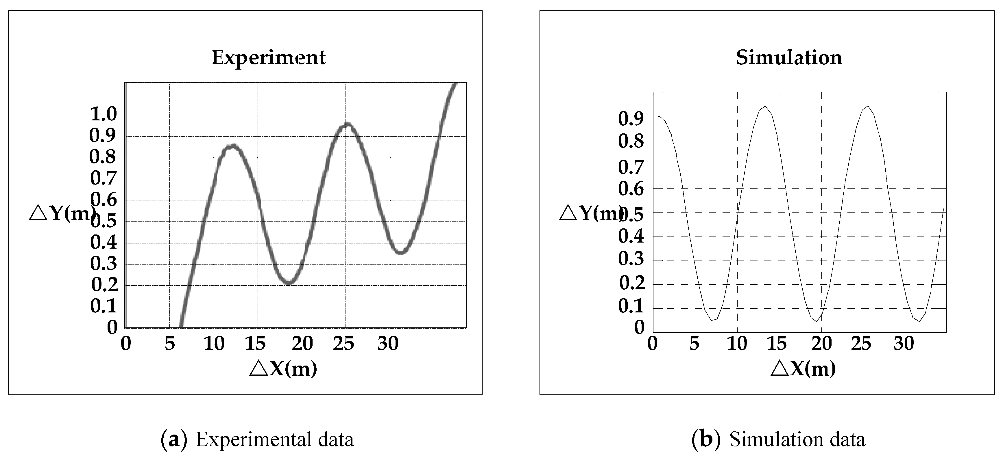
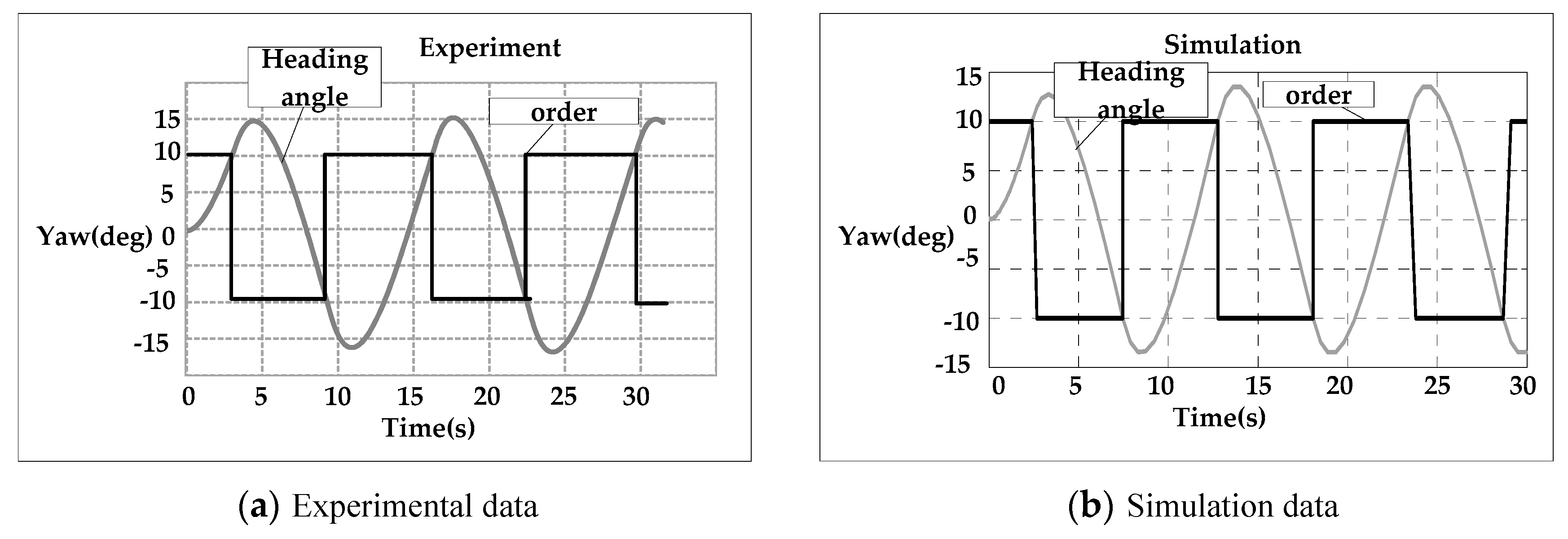
From Figure 8, it can be seen that there are some differences in ship trajectories due to the neglect of some nonlinear factors in the simulation process. There is drift in the actual experiment, but the motion characteristics and steering speed are very close. The analysis of the overshoot angle is shown in

Table 4. Analysis of the overshoot angle of the +10 deg zig-zag test.

Overshoot Angle (deg)	Experiment	Simulation	$\mathit{e}\mathit{r}\mathit{r}\mathit{o}\mathit{r}=\left|\frac{{\mathit{d}}_{\mathbf{experiment}}-{\mathbf{d}}_{\mathbf{simulation}}}{{\mathit{d}}_{\mathbf{experiment}}}\right|\times 100\%$
First time	4.81	3.95	17.88%
Second time	4.93	4.26	13.59%
Third time	4.84	4.18	13.64%

.

Through the zig-zag experiment, it can be seen that the maneuverability and steering performance of the ship model are similar to those of the actual ship. The first and second overshoot angles are very close. The international maritime organization (IMO) standard for maneuverability of the zig-zag experiment is that the first and second overshoot angles (${\delta }_1$,${\delta }_2$) shall satisfy the following conditions (32):

$${\delta }_1=\{\begin{array}{c}<{10}^{\circ }\hspace{0.17em}\hspace{0.17em}\hspace{0.17em}\hspace{0.17em}\hspace{0.17em}\hspace{0.17em}\hspace{0.17em}\hspace{0.17em}\hspace{0.17em}\hspace{0.17em}\hspace{0.17em}\hspace{0.17em}\hspace{0.17em}L/V<10s\\ <{20}^{\circ }\hspace{0.17em}\hspace{0.17em}\hspace{0.17em}\hspace{0.17em}\hspace{0.17em}\hspace{0.17em}\hspace{0.17em}\hspace{0.17em}\hspace{0.17em}\hspace{0.17em}\hspace{0.17em}\hspace{0.17em}\hspace{0.17em}\hspace{0.17em}L/V\ge 30s\\ <{\left(5+\raisebox{1ex}{$1$}\!\left/ \!\raisebox{-1ex}{$2$}\right.\left(L/V\right)\right)}^{\circ }\hspace{0.17em}\hspace{0.17em}10\mathrm{s}\le L/V<30s\end{array}\hspace{0.17em}\hspace{0.17em}\hspace{0.17em}{\delta }_2=\{\begin{array}{ll}<{25}^{\circ }\hfill & L/V<10s\hfill \\ <{40}^{\circ }\hfill & L/V\ge 30s\hfill \\ <{\left(17.5+\raisebox{1ex}{$3$}\!\left/ \!\raisebox{-1ex}{$4$}\right.\left(L/V\right)\right)}^{\circ }\hfill & 10\mathrm{s}\le L/V<30s\hfill \end{array}$$

(32)

In (32), L is the length of the ship and V is the velocity. In this test, $L/V<10s$, so both of them meet the IMO standard. In summary, the ship model can be used in simulation calculation and has a strong substitution.

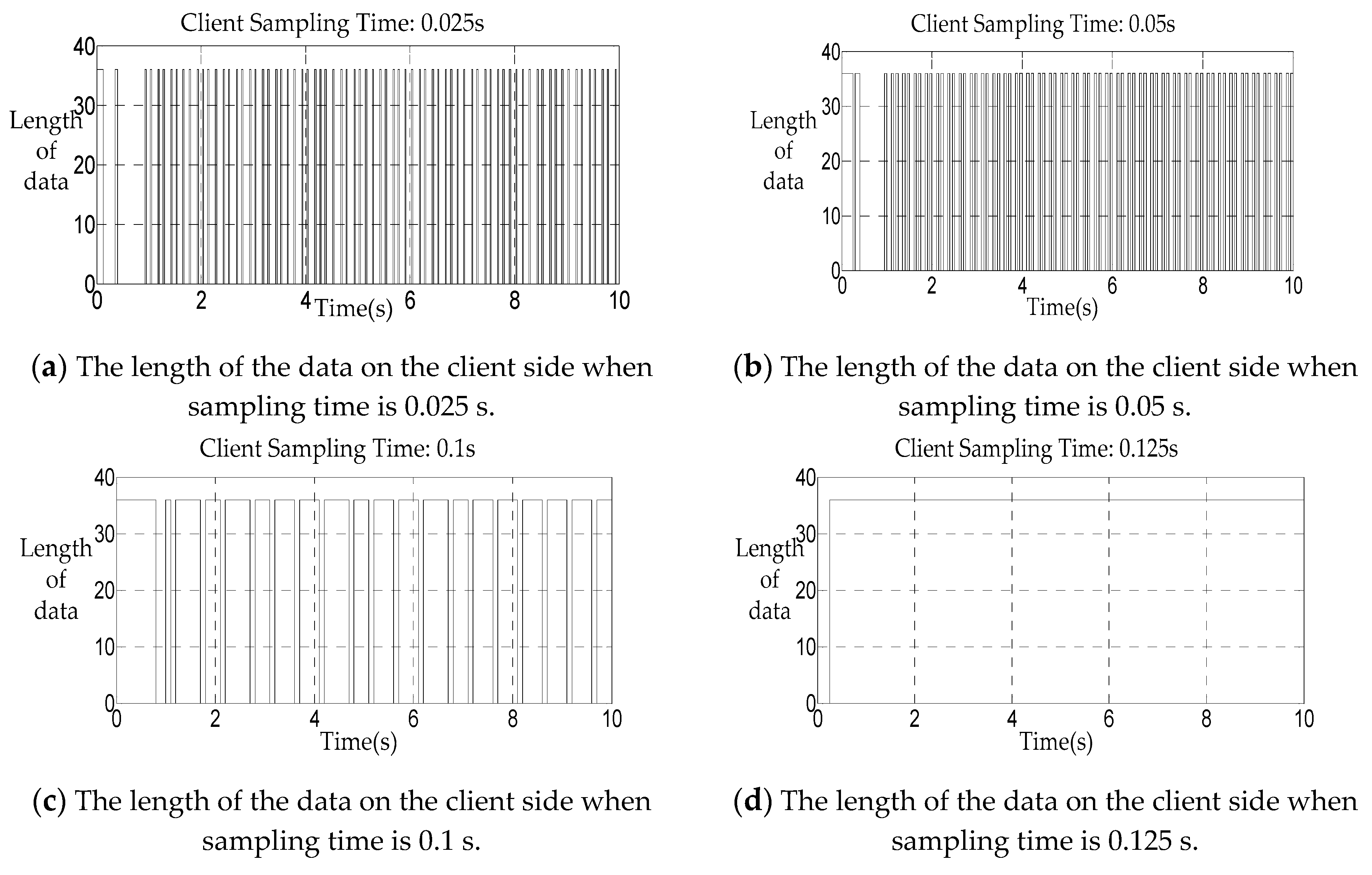
In the process of ship motion simulation, two computers were used, one functioning as a server to receive and publish ship data, and the other serving as a ship motion controller. In the actual communication process, the communication frequency of both sides is a very important factor. If the communication frequency is not appropriate, it will cause packet loss and control effect weakening. The communication frequency was tested as follows: The server issued data to the network in a period of 0.05 s, and the client was tested with 0.025 s, 0.05 s, 0.1 s, and 0.125 s, respectively. The numbers of data received are shown in Figure 10:

As shown in Figure 10, the larger the client sampling time, the smaller the data loss. When at 0.125 s, there is no loss of data, so this sampling time is used in the simulation. In addition, for the sake of insurance, a strategy is adopted in the test, that is, if there is a packet loss, the data received at the previous moment will be maintained, so as to ensure the real-time status and effectiveness of the control.

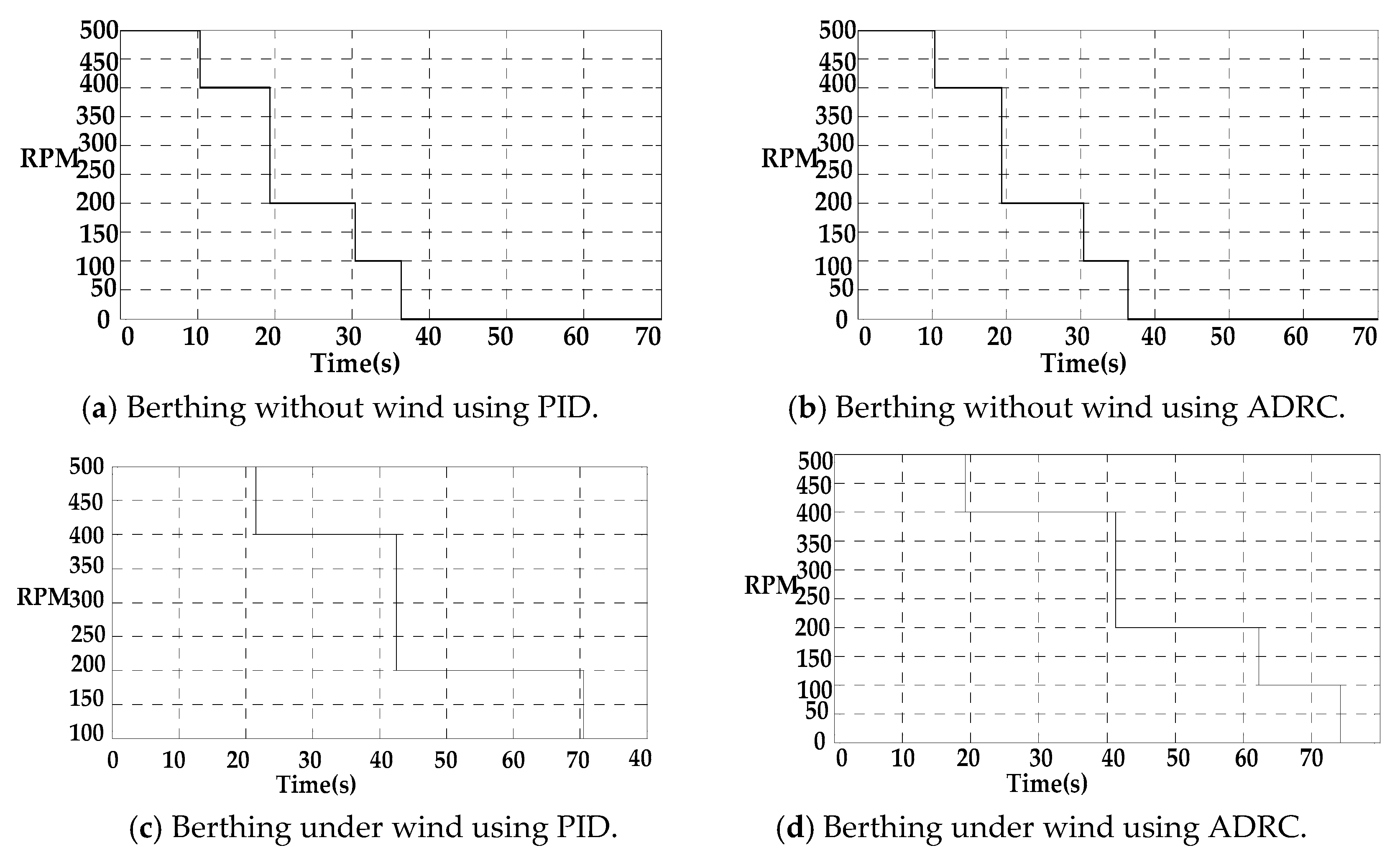
In the next step, the PID controller and ADRC controller were applied to simulate the automatic berthing of an unmanned ship. The speed control adopts the step-by-step descending mode based on actual navigation experience, and the speed changes to 0 when the specified berth arrives. Parameters of PID: 0.84; 0.001; 1.56. Parameters of ADRC: r = 100; h = 0.1; $a_{01}$ = 0.5; $a_{02}$ = 0.25; ${\delta }_1$ = 0.1; ${\beta }_{01}$ = 10; ${\beta }_{02}$ = 100; ${\beta }_{03}$ = 500; b₀ = 1; $a_1$ = 0.75; $a_2$ = 2.75; ${\delta }_2$ = 0.1; $k_1$ = 0.35; $k_2$= 0.01; ${\delta }_{01}$ = 0.1; ${\delta }_{02}$ = 0.1. The wind speed is 1.5 m/s (model scale), representing actual five-level wind.

The results are shown in Figure 11, Figure 12, Figure 13 and Figure 14. Figure 11 shows ship trajectories in automatic berthing simulation when berthing without wind using PID and ADRC and under wind using PID and ADRC; Figure 12 shows ship heading angle; Figure 13 gives the ship rudder angle; the ship RPMs are in Figure 14.

In Figure 11, it can be seen that in windless conditions, the PID and ADRC controllers can make the ship reach berth, and the control effect is excellent. However, in the case of wind with a speed of 1.5 m/s (model scale), the ADRC controller makes the ship trajectory more stable, and the ship arrives at berth smoothly. The PID controller has a poor control effect, which makes the ship only reach the edge of the berth. In Figure 12; Figure 13, it can be seen that ADRC has a more sensitive steering ability than PID. In Figure 14, we can see that the speed can be adjusted according to the distance, and the ship can be parked in the designated berth. Detailed analysis is in

Table 5. Analysis of the results of simulation of ship automatic berthing.

	Heading Adjustment Time	RPM Zero Time	D	Y/N
(a)	29.5 s	36.2 s	0.4 m	Y
(b)	22.3 s	35.8 s	0.5 m	Y
(c)	55.4 s	71.4 s	1.7 m	N
(d)	52.3 s	73.5 s	0.6 m	Y

, where (a) is for berthing without wind using PID, (b) is for berthing without wind using ADRC, (c) is for berthing under wind using PID, (d) is for berthing under wind using ADRC. D is the distance between the final position and the center of the berth, while Y/N is whether to complete automatic berthing.

As can be seen from Table 5, the heading adjustment time is the time when the course reaches relative stability, and that of ADRC is faster than that of PID in each case. It should be considered that ADRC can make the ship react more quickly. RPM Zero Time is the time when the ship arrives at the berth. In the case of wind, the speed of the ship is slowed down and the adjustment time is longer, and the PID controller makes the ship reach the edge of the berth. Although the speed can be 0 at this time in the simulation strategy, this situation is considered to be the failure of automatic berthing in practice. Whether with an ADRC or PID controller, the strategy of frequent steering is used to resist the influence of wind on ship motion in the case of wind, and the effect of ADRC is better.

5. Automatic Berthing Experiment

The tank experiment was carried out at the Japan National Research Institute of Fisheries Engineering, and the plane scale coordinate schematic diagram of the experiment is shown in Figure 6. The experimental system of a self-propelled ship model includes a scale ship model, self-propelled mechanism, communication system, camera, positioning and orientation system, speed sensor, etc. In this experimental system, the ship position was obtained by the ultrasonic positioning system, and the heading angle was measured by the fiber optic gyroscope on the ship, and the speed of the ship was measured by the anemometer at the bottom of the ship. All ship navigation data were stored in the ship’s microcomputer and sent to the shore data exchange server (DES), which is similar to the function of the ship’s automatic identification system (AIS). An initial setting server sends initial configuration information to ships through Bluetooth. DES sends ship dynamic data to the control system and receives control commands (rudder angle and propeller speed) and sends them to the corresponding ship model. 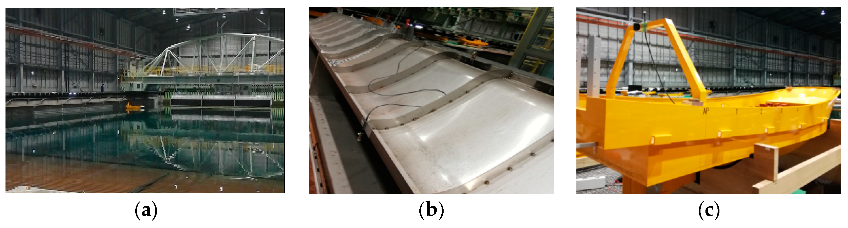Figure 15 is a photograph of the experiment tank, wind-making machine, and ship model.

Because speed control is easy to achieve, in this experiment, the speed of the propeller was kept at a very low speed. The speed of the propeller was maintained at 60 rpm, and the speed of the propeller was 0 after the ship reached the target berth. According to the parameters used in the simulation, the parameters of the controller were adjusted through field experiments. The results of PID: 0.6; 0.001; 1.2. ADRC are as follows: r = 100; h = 0.2; $a_{01}$ = 0.5; $a_{02}$ = 0.25; ${\delta }_1$ = 0.1; ${\beta }_{01}$ = 5; ${\beta }_{02}$ = 30; ${\beta }_{03}$ = 70; b₀ = 1; $a_1$ = 0.75; $a_2$ = 2.75; ${\delta }_2$ = 0.1; $k_1$ = 0.35; $k_2$= 0.01; ${\delta }_{01}$ = 0.1; ${\delta }_{02}$ = 0.1. In this experiment, there are four typical cases for comparative analysis.

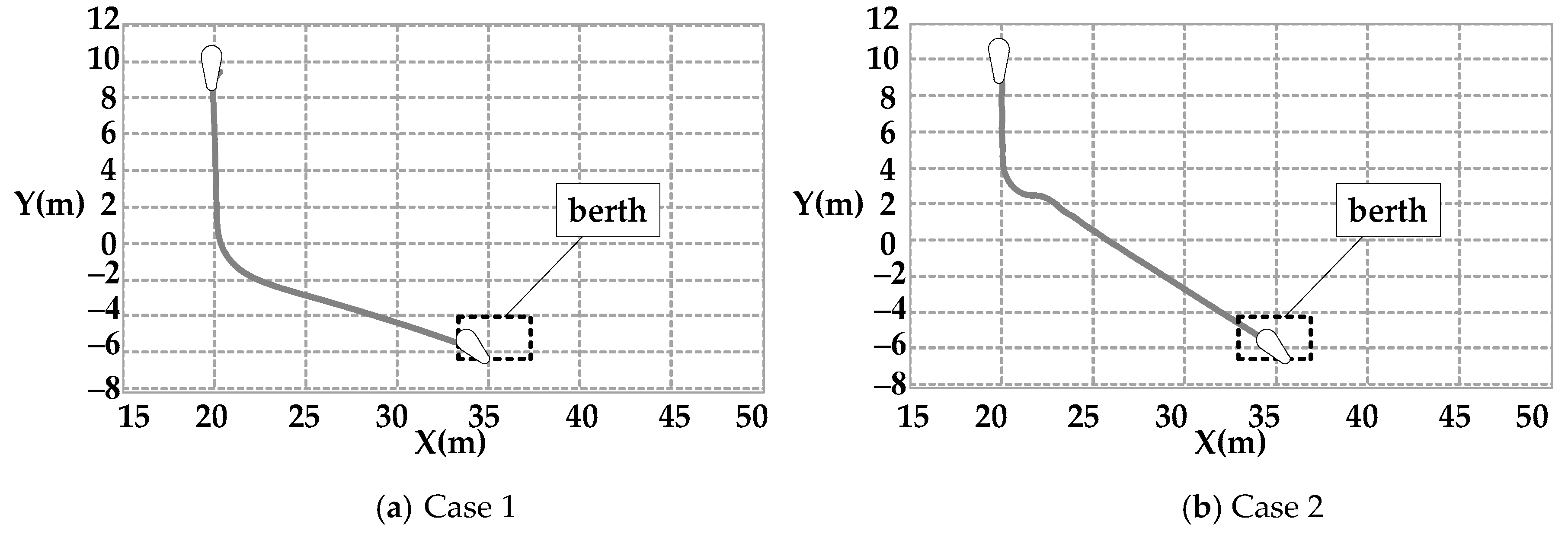
Case 1: The controller uses the PID algorithm, and the experiment was completed without wind disturbance.

Case 2: The controller uses the ADRC algorithm, and the experiment was completed without wind disturbance.

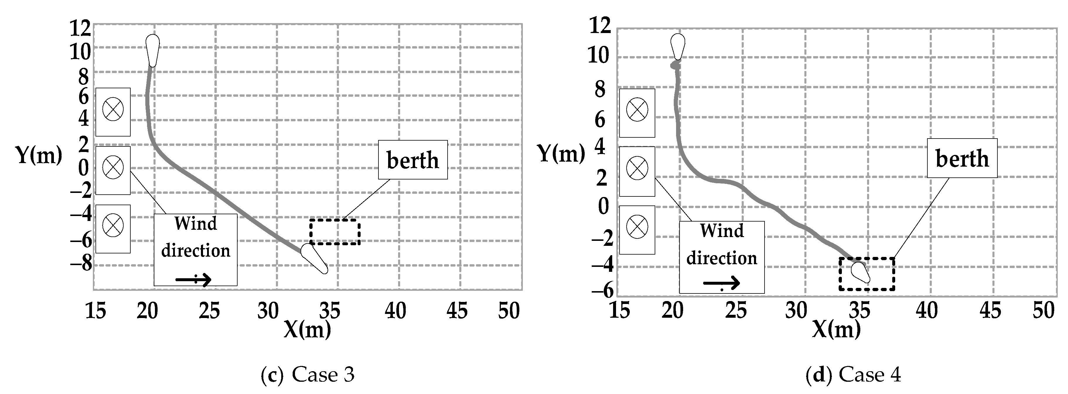
Case 3: The controller uses the PID algorithm, and the experiment was completed with wind whose speed was 1.5 m/s (model scale), representing actual five-level wind.

Case 4: The controller uses the ADRC algorithm, and the experiment was completed with wind whose speed was 1.5 m/s (model scale), representing actual five-level wind.

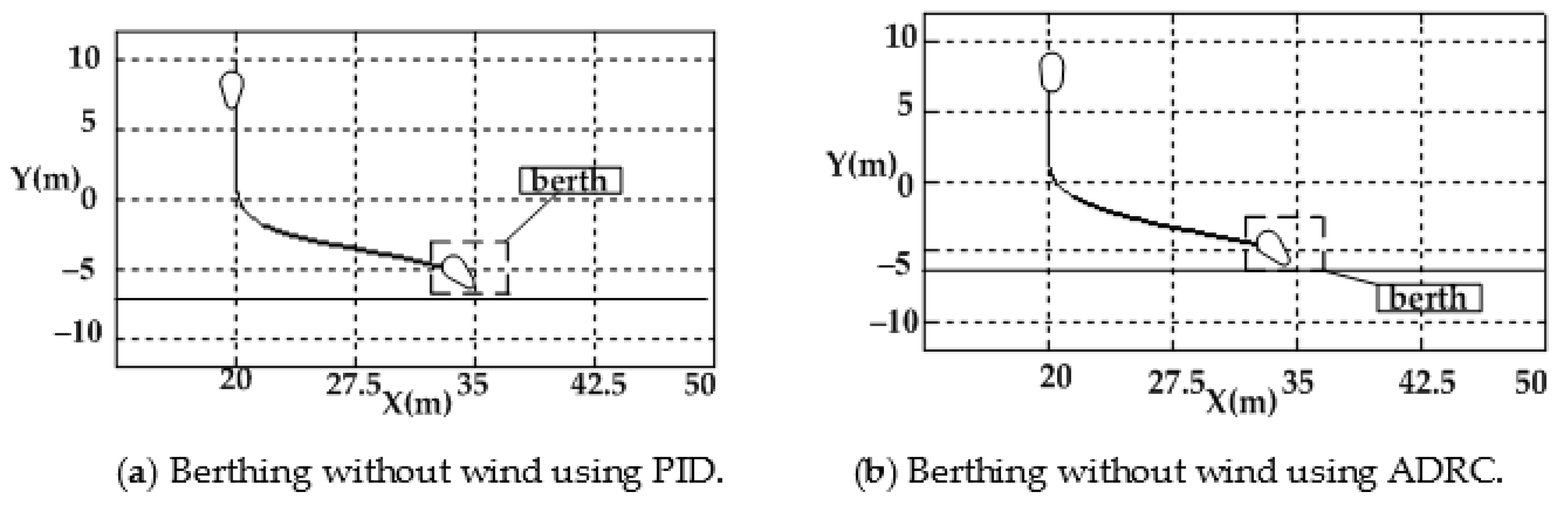
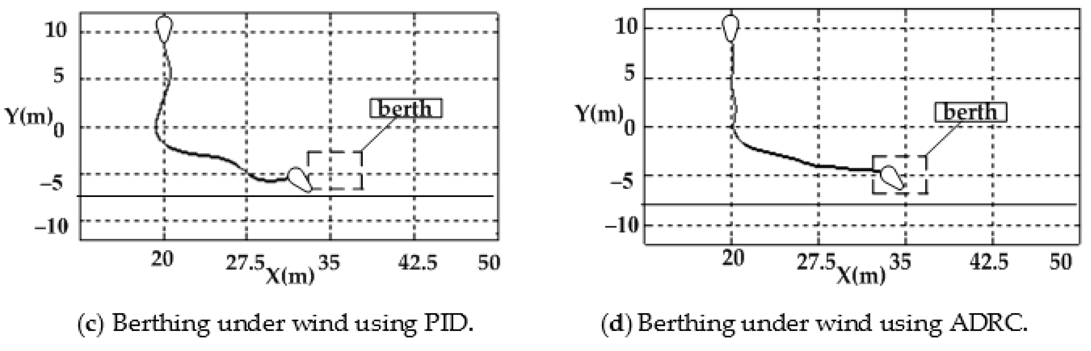
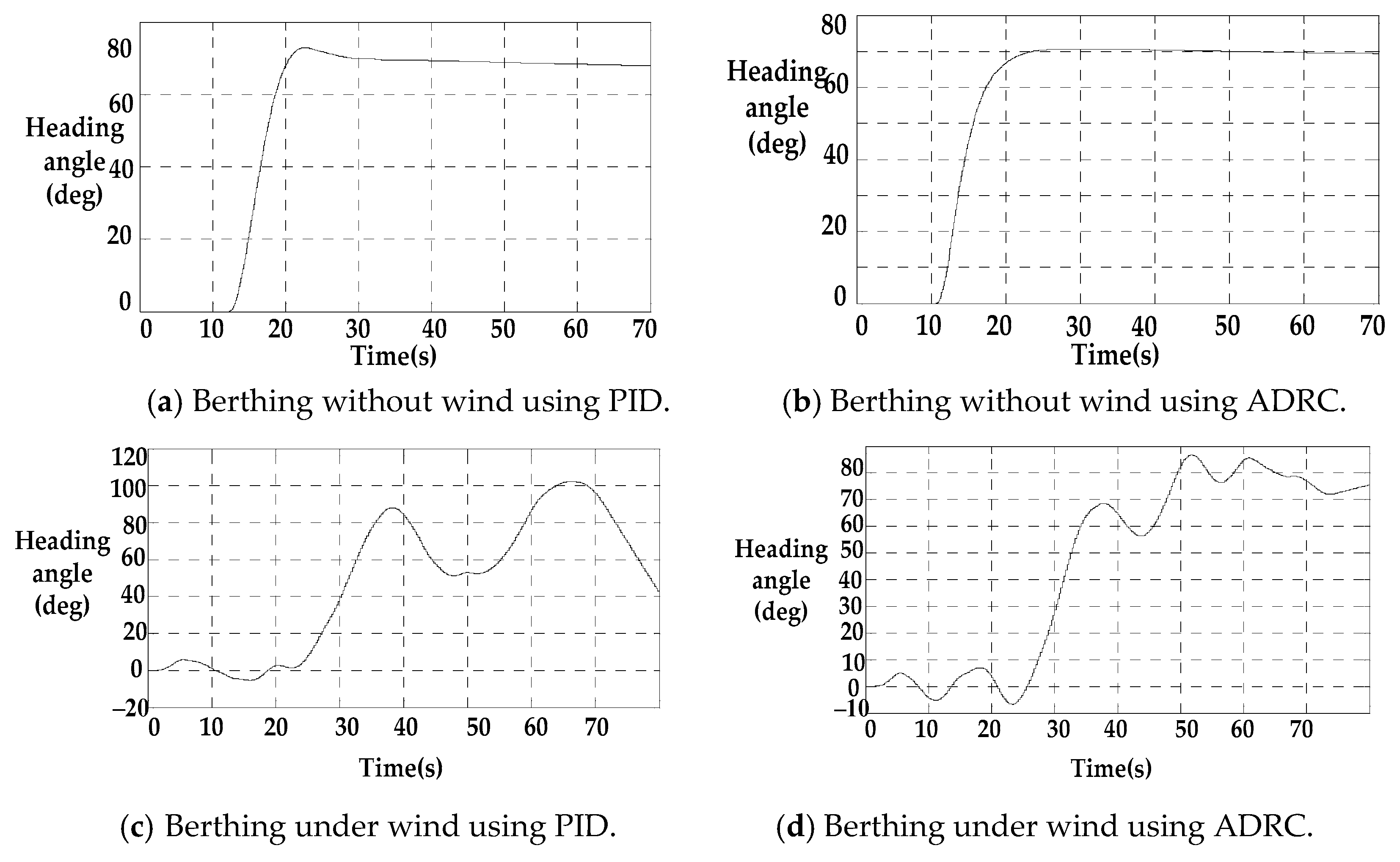
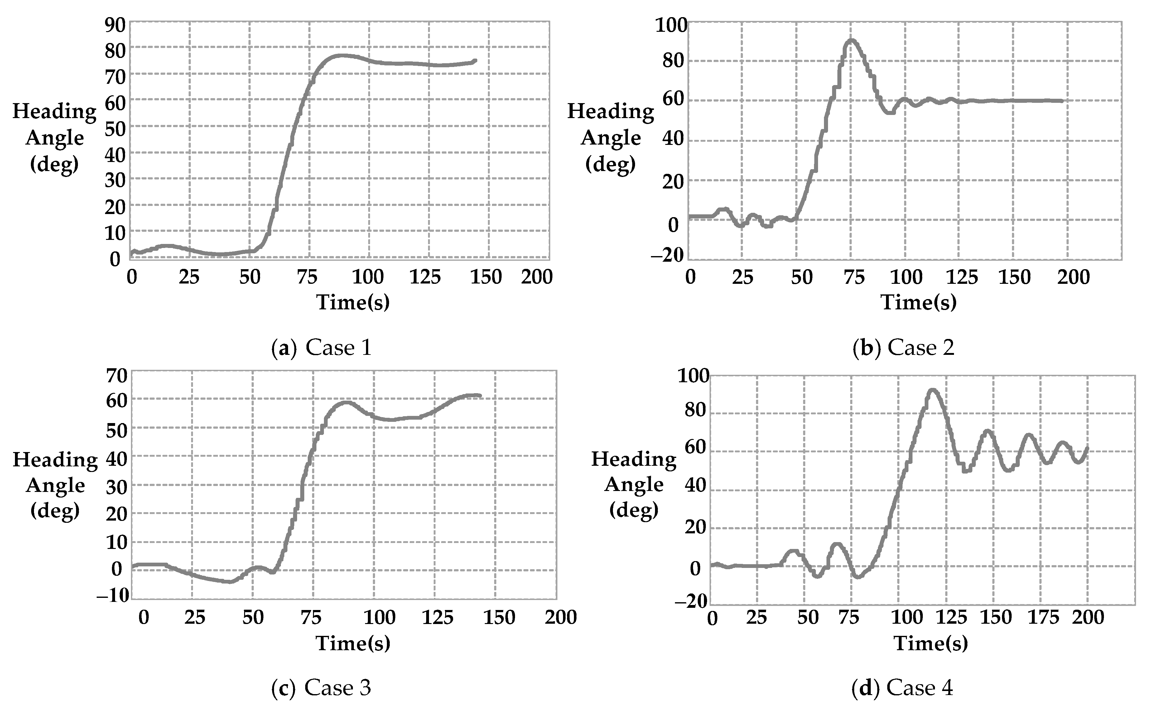
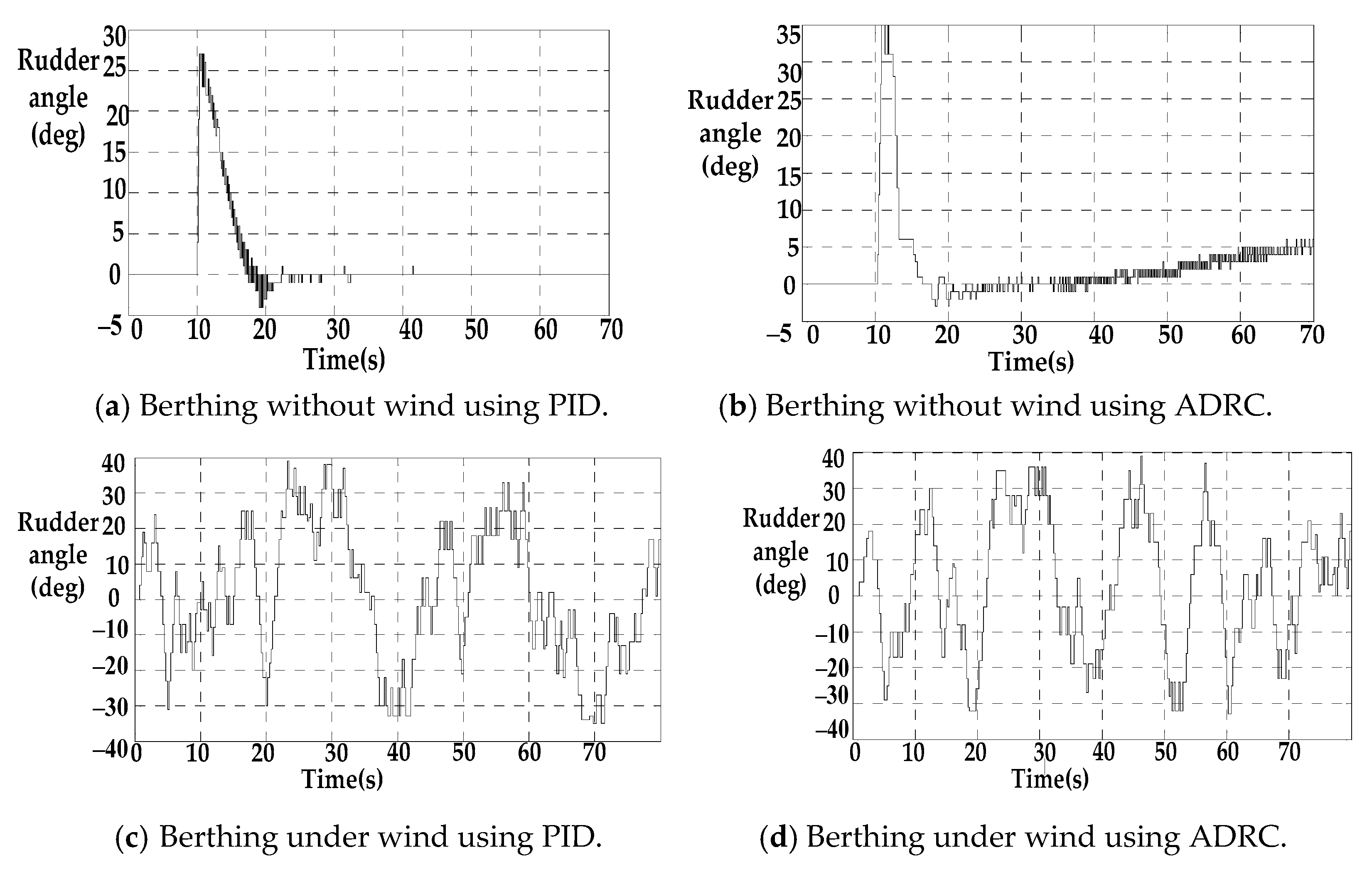
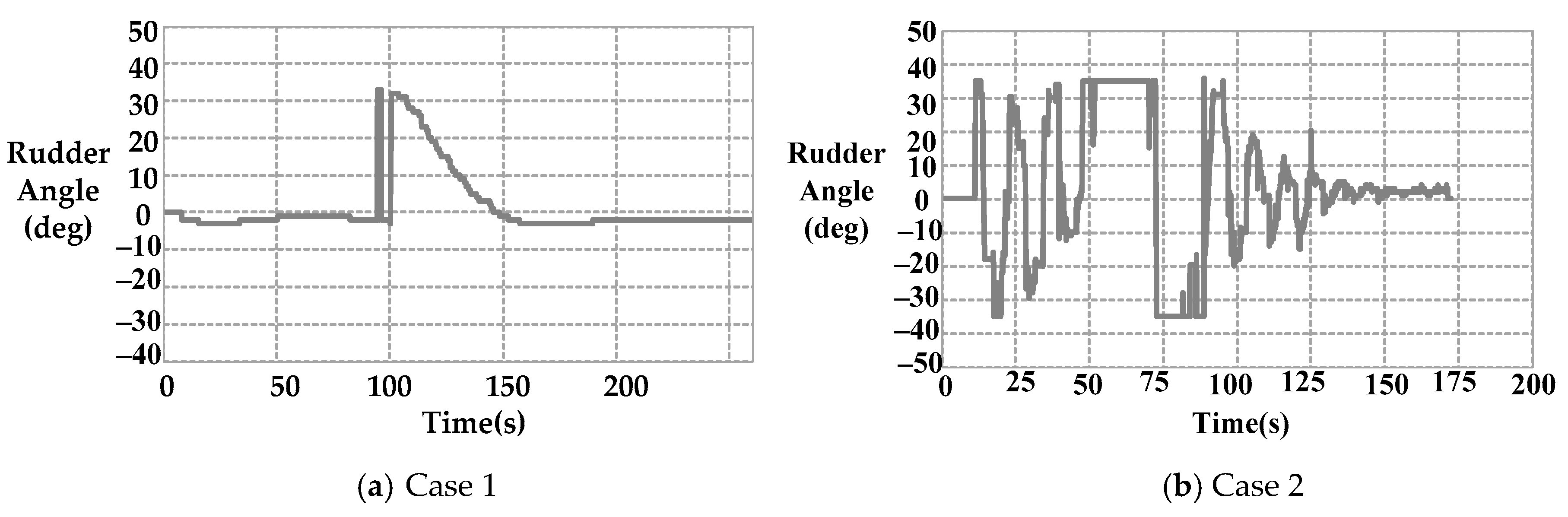
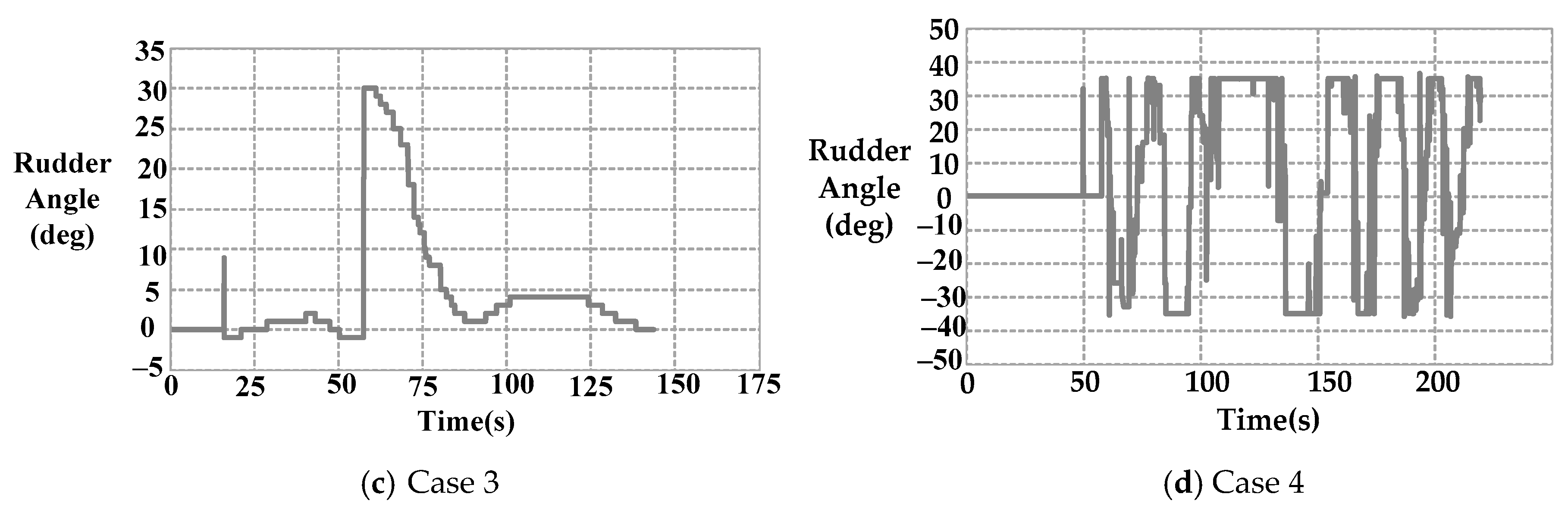
The experimental results are shown in Figure 16, Figure 17 and Figure 18. Figure 16 shows ship trajectories in the tank experiment of ship automatic berthing when berthing without wind using PID and ADRC and under wind using PID and ADRC; Figure 17 gives the ship heading angle; Figure 18 shows the ship rudder angle.

From the above results of Figure 16, Figure 17 and Figure 18, it can be seen that the unmanned ship can reach the target berth smoothly without wind using the PID controller. From the above results of case 2, it can be seen that the ADRC controller can also achieve the desired control effect, but the nonlinear compensation structure of the controller makes the rudder angle change frequently because it is sensitive to the surrounding conditions. The effect of this wind level on the autonomous navigation of unmanned ships is more serious, especially at low speed, because the effect of the rudder is weakened. From the above results of case 3, due to the effect of wind, it is difficult to steer, the ship reacts slowly, and the rudder’s function is mostly due to disturbance resistance, which results in the unmanned ship deviating from the target course and not reaching the designated berth completely. From the above results of case 4, under the action of wind, ADRC has a faster response ability. Because of the existence of TD and ESO, unmanned ships can make faster turns due to the prejudgment and excessive disturbance. Despite the frequent changes of rudder angle, the scheduled berth is reached, which solves the problem that the rudder effect of the unmanned ship is weakened and deviates from the course due to strong wind. Detailed analyses are in

Table 6. Analysis of the results of the experiment of ship automatic berthing.

	Heading Adjustment Time	Time of Arrival at Berth	D	Y/N
Case 1	105.2 s	130.3 s	0.8 m	Y
Case 2	98.4 s	134.5 s	0.3 m	Y
Case 3	110.5 s		2.7 m	N
Case 4	123.5 s	148.1 s	0.6 m	Y

. D is the nearest distance to the center of the berth, and Y/N is whether to complete automatic berthing.

From Table 6, we can see that the results of the experiment are close to those of the simulation, but the adjustment time becomes longer because of the low-speed navigation and the lack of control over RPM in the experiment. In the experiment, it was found that in the case of wind, ship steering becomes more difficult, especially in the case of low speed, and when the wind speed is high to a certain extent, the ship cannot even steer, so it is of great value to design a better controller under reasonable circumstances. In case 3, the ship fails to pass the berth, and the effect of wind on the result is greater than that in simulation. The control results of cases 1 and 2 are similar, and the ship has successful automatic berthing. The experiment results show that the berthing controller using ADRC is effective, with more appropriate initial parameters and a better control effect. Moreover, the control is still effective in the presence of wind disturbance, which shows that the controller is insensitive to external disturbance and has a certain robustness. In general, the disturbance of wind in the berth of the wharf is relatively small, so the controller can resist such disturbance to achieve the control task.

6. Conclusions

Through this experiment, the effectiveness of the ADRC algorithm, when used in the automatic berthing of an underactuated unmanned ship under wind loads, was verified. This paper mainly draws the following conclusions:

(1) In the process of automatic berthing of unmanned ships, the LOS algorithm is a reliable algorithm. The algorithm is simple and easy to implement, which lays a foundation for further ship motion control.

(2) The mathematical model of ship motion established in this paper has been verified by maneuverability simulation tests. The results obtained by simulation were basically similar to those obtained by experiments and have reference value.

(3) The ADRC algorithm accelerates the ship’s response to the disturbances by changing the rudder angle frequently when permitted. It further proves that the intelligent control algorithm can improve the control effect of an unmanned ship.

(4) Through the comparative analysis of experimental results and simulation results, we can see that the situation in the experiment and simulation is not exactly the same. In the actual experiment, there are more nonlinear and unknown factors affecting ship motion. In future simulation analysis, more detailed and comprehensive considerations are needed.