Stochastic Modeling of Forces on Jacket-Type Offshore Structures Colonized by Marine Growth

Abstract

The present paper deals with the stochastic modeling of bio-colonization for the computation of stochastic hydrodynamic loading on jacket-type offshore structures. It relies on a multidisciplinary study gathering biological and physical research fields that accounts for uncertainties at all the levels. Indeed, bio-colonization of offshore structures is a complex phenomenon with two major but distinct domains: (i) marine biology, whose processes are modeled with biomathematics methods, and (ii) hydrodynamic processes. This paper aims to connect these two domains. It proposes a stochastic model for the marine organism’s growth and then continues with transfers for the assessment of drag coefficient and forces probability density functions that account for marine growth evolution. A case study relies on the characteristics (growth and shape) of the blue mussel (Mytilus edulis) in the northeastern Atlantic.

1. Introduction

Actual challenges for requalification of existing offshore structures through the reassessment process emphasize the importance of updating information about the structural condition state. One of the most important phases during the design or re-assessment level is a re-evaluation of environmental loads and updating knowledge concerning the state of biocolonization, structural damage, and corrosion. The random nature of biofouling and the uncertainty inherent to biological processes make modeling of environmental loading complicated. Biofouling is a complex phenomenon involving a diversity of marine species, which constitute communities whose dynamic is driven by physical and biological processes. It has many negative impacts on offshore structures such as loading excess, structures occlusion, increase in drag coefficient, and corrosion [1,2]. Therefore, it represents a challenge for engineers with respect to design and maintenance programs. Several standardized methods of inspections and in-situ measurements of the marine growth have been developed to obtain relevant information about species composition, percent cover, weight, thickness, and roughness, allowing the determination of structural design, cleaning, and maintenance strategies. Biocolonization processes show spatial and temporal variations related to several environmental factors (water temperature, hydrodynamics, turbidity, distance from the shore, bottom characteristics) acting at regional and local scales. However, the results are often more qualitative than quantitative and suffer from a lack of consistent modeling for structural engineers, except when a big database is available. Cost-effective, safety management of offshore structures involves allocating the optimal amount of resources to periodical inspections and maintenance activities in order to control risks (expected life of the structure).

The growth of marine organisms on offshore structures has long been a significant issue for the oil and gas industry [1,2]. In the 70′s and 80′s, studies focused on the effect of biofouling on hydrodynamic forces acting on offshore structures. Numerous experimental studies were carried out with different types of marine growth, cylinder diameter, and hydrodynamic conditions to provide a better understanding of their interactions with hydrodynamic forces and to highlight the key relationships. Despite the great variability due to the complexity and instabilities of the flow regime around structures, abacuses were built and are still recommended by offshore standards such as American Petroleum Institute (API) [3] and Det Norske Veritas (DNV) [4]. Only a few studies considered the global modeling of the loading in a probabilistic context [5,6] and none of them consider the modeling of the organismal growth itself. In fact, there are few available databases containing on-site measurements with time [7,8]. This paper proposes a modeling of characteristics of the external marine growth layer consistent with structural engineering needs. As the first year is crucial for future colonization patterns, we focused here on the building of the first layer of biofouling by a macro-fouler. The blue mussel Mytilus edulis was considered for the modeling, as it is an ubiquist bio-fouler in European waters [9,10].

The present paper considers the biocolonization as a stochastic process. Biocolonization is represented as cumulative deterioration process and this study defines two phases for it: an initiation phase and a propagation phase. The paper reviews meta-models and it describes database construction, which consists of the influencing factors. It proposes a stochastic modeling of biofouling based on a non-stationary, state-dependent Gamma process for the blue mussel Mytilus edulis. The developed Gamma process [11,12] provides individual shell length time series for blue mussels in the first year of colonization. Its parameters are identified from simulations carried out by a biological model. To this aim, a biological model based on the Dynamic Energy Budget (DEB) theory [13,14] was used to simulate the variations of individual mussel shell size depending on environmental data. Thereafter, the study focuses on the drag term of Morison’s equation. It reviews a response surface method to model the drag force as well as the effect of physical characteristics of structural members, such as surface roughness (k) and the average thickness of marine growth (Th). Moreover, the drag force exerted by extreme waves for colonized structural members during the typical macro-colonization years is determined. The probabilistic macro-colonization, shell length time-series considering the occurrence probability of typical macro-colonization years are provided. The evolution of the drag coefficient with regard to the probabilistic shell length time series is evaluated and the results are discussed.

A case-study site was chosen offshore the Loire Estuary (France) corresponding to a future offshore wind farm site, in order to illustrate the role of biofouling on the computation of hydrodynamic forces (drag force). In order to model the colonization during the first year, two main phases of bio-colonization were considered: (1) an initiation phase without any macro-fouling on the structure, and (2) a propagation phase or macro-colonization phase, corresponding to the growth of mussels. The key influencing factors affecting these two stages were hydrological data (water temperature and chlorophyll-a concentration, as proxy of mussel food). Mussel growth was used to derive two geometrical characteristics Th and k describing marine growth. It should be noted that the added mass and inertia forces are beyond the scope of this paper.

Hereafter, the objective of this work is to propose a meta-model, which combines different disciplinary approaches accounting for several types of uncertainty and variability among (a) the temporal variability of the main influencing environmental factors; (b) the biological uncertainty of the individual’s growth; (c) the uncertainty, due to the modeling of geometrical parameters of structural components caused by biofouling and needed for structural computations; and (d) the uncertainty of wave characteristics to compute the loading on structural components. To propagate the uncertainty of biological and physical marine environment (marine growth and wave), a physical matrix response surface was used in view to provide a probabilistic model of the environmental loading on jacket type offshore structures based on Schoefs & Boukinda (2010) [1]. This method was applied for quasi-static calculations of wave forces in the presence of marine growth.

2. Materials and Methods

2.1. Requirements for a Meta-Model

To develop the macro-colonization model for structural computation, several properties should be considered. The main trends of growth with time should be captured using a time step compatible with sensitivity to input parameters; it should be sensitive to the environmental parameters that govern the ecophysiology of the biofouling: temperature and food availability; it should provide intermediate parameters (shell size) from which required outputs can be easily computed (roughness and thickness) to perform a reliability analysis (stochastic processes); it should be versatile to modify the trends depending on site specificity. The next sections detail the way these requirements have been taken into account in this work.

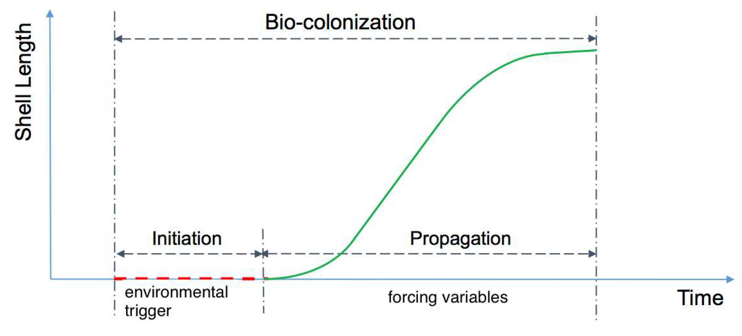
2.2. Description of Bio-Colonization Temporal Dynamic

Bio-colonization is a complex process depending on biotic and abiotic variables with many interactions [15,16]. Indeed, it would be unrealistic to envisage a complete model involving a multilayer of various marine organisms that have complex interactions for survival, growth, and reproduction. We propose here a model that accounts for the temporal variability of the main influencing factors in a simplified but realistic case. It focuses on the growth of a single species, the blue mussel Mytilus edulis.

The bio-colonization process depends on two early stages: (1) the reproduction of adults, which spawn in the water column and produce larvae that will become part of the plankton transported by currents; (2) larval survival and development in the water column. The bio-colonization itself starts with the larval settlement on a structure (micro-colonization) and corresponds mainly to the macro-colonization step, i.e., growth of individuals up to the adult state. It is important to estimate the spawning date(s) and to assess the conditions allowing larval survival. This is a prerequisite before modeling macro-colonization. Consequently, the model needs to take into account (1) an initiation phase (no macro-organism present on the structures) with no significant effect on structural reliability, and (2) a propagation phase corresponding to the growth of macro-organisms (Figure 1). With these two phases, an analogy can be made with the dynamic of degradation processes like corrosion of steel rebars in reinforced concrete [17]. In this study, we considered that the larval settlement corresponds to the beginning of the propagation phase.

The model should be able to capture the initiation phase and then simulate a propagation phase (macro-colonization). The latter allows for obtaining the individual size and, accordingly, the physical characteristics of the colonized surface needed for the hydrodynamic calculations [6]. The initiation phase includes spawning date, larval survival, development, and settlement. We considered that this phase was mainly driven by temperature while the propagation phase (macro-colonization) corresponding to the juvenile growth was driven by both, the temperature and the concentration of chlorophyll-a, a proxy of the food available in the water column for mussels. These drivers are related to the bivalve ecophysiology, which is detailed in the following paragraph.

2.3. Description of Bio-Colonization Temporal Dynamic

The blue mussel Mytilus edulis (M. edulis) was chosen to develop a simplified (single organism colonization) but realistic bio-colonization model for the North-Atlantic coasts. M. edulis is a ubiquitous and abundant species in the coastal waters of the North and Mid-Atlantic Regions [18], and has been reported as a main macro-colonizer of offshore structures [19,20]. When found as a dominant hard fouler, it has an influence on the composition of the external layer of marine growth [15]. It is a suspension-feeding bivalve that attaches to substrata by byssal threads and is traditionally cultivated on ropes or wooden poles on the Western Atlantic coasts [21]. M. edulis is eurythermal (adaptable to a wide range of temperatures) and, under the latitude of our case-study site, is well acclimated to a 5 to 20 °C temperature range [22]. It is very common in the intertidal area forming beds on rocky and hard substrates but can be found in subtidal environment down to −10 m. Mussels feed on suspended particulate matter and their main food resource is phytoplankton cells [23,24,25]. Phytoplankton is also considered as the dominant food source for all life stages of M. edulis since larvae also rely on phytoplankton for their development. The concentration of chlorophyll-a is a widely used proxy of phytoplankton biomass, and this variable was used in this study to assess the food available for the mussel’s growth. For more details on M. edulis morphology, physiology and ecology, the reader is referred to Gosling (2003) [21].

2.4. Initiation Phase and Propagation Phases

The spawning date, larval survival, and development are the most important stages for the initiation phase modeling. Blue mussels, like the majority of shallow water bivalves, produce large numbers of pelagic planktotrophic larvae that spend several weeks in the surface waters [25]. M. edulis sexes are separated, and gametes are shed into the water where fecundation occurs. At the latitude of the study site, mussels can spawn up to three times a year from April to September successively, depending on environmental factors. In bivalves, an essential condition related to spawning is a thermic threshold corresponding to a minimum water temperature [26]. Indeed, the temperature is the strongest exogenous factor controlling M. edulis reproduction [21]. In this work, we considered only the spring period when the mussel producers submerge ropes to collect planktonic larvae. In Pertuis Breton, which is the closest area to our study site, Barillé-Boyer (1996) [22] found a threshold of 10.5 °C, and it has been considered that spawning was not triggered below this temperature. Above this temperature, the spawning dates are not modeled but forced with observed datasets [24]. In this study, observations from mussel producers are used. A 30 day interval between two spawning was adopted in relation to the mussel gametogenesis dynamic. This delay is linked to the time necessary to reconstitute reproductive tissues [22]. Other exogenous factors, such as storms, shock, rain, etc., which can randomly trigger bivalve’s spawning, were not considered. The second important step following spawning is the larval survival and development. For mussels, Bayne (1965) [27] observed that M. edulis larvae could reach its development within 20 to 40 days, depending on the temperature. A slower (S) larval growth and metamorphosis can take 40 days if spawning happened in early spring with a water temperature of around 10 °C, while a faster (F) larval development of around 20 days is possible at a higher temperature of 14 °C [22]. Therefore, it was considered that if during the next 20 days after spawning water temperature was >14 °C, larvae survival and development was completed in 20 days, otherwise in 40 days. For each year in our database, the spawning occurrence times and initiation phase typologies are determined by post-processing the temperature time-series.

As mentioned before, geometrical parameters (thickness and roughness) are required for load computation. They depend on geometrical specifications (shape) of organisms colonizing the structure. In this study, these parameters are linked to the shell length of blue mussel individuals. The shell growth of the blue mussel has an asymmetric sigmoid shape curve [28,29]. The growth rate of blue mussel individuals is, therefore, neither monotonic nor stationary, and the growth curve can be described by the acceleration and deceleration phases (Figure A1, in Appendix A). No clear relationship between the individual shell growth and the water temperature has been observed, while the concentration of chlorophyll-a appeared to be the main driver. This observation is consistent with several studies showing that the food supply was the most important variable explaining mussel growth [30,31,32].

2.5. Database Post-Treatment, Virtual Database, and Aggregation of Influencing Factors

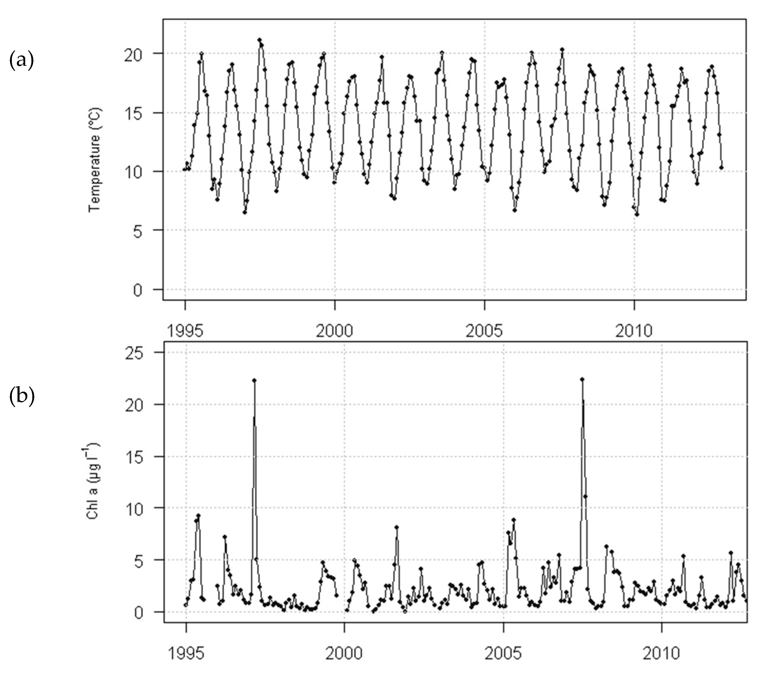
2.5.1. Environmental Data at the Case-Study Site

In order to model the initiation and propagation phases, water temperature and chlorophyll-a (Chl. a) concentrations were obtained for the site of Le Croisic (47°17′33″ N, 2°31′15″ W) on the western Atlantic coast of France. This location was chosen for its proximity to the future offshore wind farm site of Banc de Guérande (47°19′41″ N, 2°25′46″ W). Data were collected by the French Observation and Monitoring program for Phytoplankton and Hydrology in coastal waters (REPHY, [33]), and implemented and managed by the French Research Institute for the Exploitation of the Sea (Ifremer). Bimonthly samples were collected at a sub-surface depth (between 0 and 1 m) during high tides between 1996 and 2012 (Figure 2). Chlorophyll-a display higher concentration between March to June corresponding to the spring phytoplanktonic bloom characteristic of northern hemisphere temperate waters. In 2004, a single spring peak was observed, while in 1996, three peaks of lower concentrations were detected. It should be noted that the water temperature cannot change abruptly in a short time. For an overview of the REPHY network, the reader is directed to Hernández Fariñas et al. (2013) [34].

In order to model bio-colonization and to standardize the time intervals of data acquisition, each month has been divided into three 10 day periods. The database used hereafter has been therefore constructed from periodic observations at established time intervals τ equal to 10 days. The average value of all temperatures and Chl. a values measured during each decade has been assigned as the decade temperature and Chl. a values. It should be noted that the water temperature cannot change abruptly in each decade. On the other hand, Chl. a will not interfere directly in the model but rather will form the growth potential parameter that is explained in next section. That is why if there were no available measurements available for some decades, a linear interpolation from adjacent measurements was carried out. The number of the database time-series [Year Time-step] is defined by N, representing the number of years for which the database base has been prepared, and t, which represents the number of observations each year depending on the data acquisition time intervals (in days) τ; in our case N = 17, t = 37 and τ = 10. The long-term time-variant modeling of input factors being out of the scope of this work, we assumed that N is statistically sufficient for computing the frequency of each macro-colonization scenario. Therefore, the database has been constituted from the regular measurements of water temperature (T) and Chl. a (C), and can be denoted as:

$$\left\{\left(T_{t,\tau }^i,C_{t,\tau }^i\right);t>0,i\in 〚1,N〛\right\}.$$

(1)

Hereafter, Tⁱ_t,τ, is used for the initiation phase determination and Cⁱ_t,τ for the modeling of the propagation phase. Four types of larval development combining the slow (S) and fast (F) growth possibilities are presented in the

Table 1. Inter-annual development types for three main spawning events (S: slow initiation phase, F: fast initiation phase).

Development Type	Occurrence	Probability
SSS	2	0.12
SSF	10	0.59
SFS	0	0.00
SFF	5	0.29

for the three initiation times (corresponding to the three spawning periods) obtained from the database considering key factors and thresholds described in the previous section. The first larval development is always slow because the water temperature is below 14 °C during early spring, and the third one can be slow only if the second one is also slow (because the water temperature cannot fluctuate abruptly). These results come from the natural seasonal variations of temperature during one year. These frequencies will be considered as discrete probabilities for the modeling. At the end of this larval growth period, we considered that larvae settled on the structures, and that was the start of the propagation phase (macro-colonization) described in Table 1 for the 17 annual chronicles.

Table 2. Date of start of macro-colonization, expressed in 10 day periods, for three main spawning events of blue mussel.

Start of Macro-Colonization			Occurrence	Probability
11	14	15	2	0.12
11	14	17	2	0.12
11	15	16	1	0.06
12	15	16	3	0.18
13	14	17	1	0.06
13	16	17	3	0.18
14	15	18	1	0.06
14	17	18	1	0.06
15	16	19	2	0.12
16	17	20	1	0.06

shows the date of start of macro-colonization, expressed in 10 day periods (1 = first 10 days of January), for three main spawning events of blue mussel between March and June. Occurrence and probability were calculated from the 17 year time-series of temperature data at the study site. Calculations revealed that macro-colonization starting date spanned from the 11th to the 20th 10 day period. The most probable macro-colonization inception times for the three spawning events corresponded to the combination of 10 days periods of 12-15-16 and 13-16-17 with 18% probability. The first macro-colonization inception occurred between the 11th and the 16th 10 day periods with the highest probability of 29% for 11th period and the lowest probability of 6% for the 16th period. The second macro-colonization inception occurred between the 14th and 17th periods with the lowest probability of 12% for the latter. The third macro-colonization inception occurred between the 17th and the 20th periods with the highest probability of 35% for the 17th period and the lowest (6%) for the 20th.

2.5.2. Environmental Data at the Case-Study Site

There was no observation available for blue mussel shell lengths close to our study site and more generally, no database for the annual growth of mussels during the considered 17 year period. To fill this gap, we applied a bioenergetics growth model to simulate the individual shell length using environmental time-series data available at the study site. This biological model was calibrated by a site with similar environmental characteristics and for the same species of mussels. Different bioenergetics models have been developed to model the growth of bivalves depending on the environmental conditions, and among them, Dynamic Energy Budget (DEB) models [13] have been successfully applied to several bivalve species [24,35,36,37,38]. DEB models do not use empirical allometric relationships, but simply state that feeding is proportional to surface area, whereas maintenance is scaled according to structural body volume [13]. DEB theory proposes a generic energy budget approach that assumes common physiological processes among species and life stages via a set of parameters, the only difference among species lying in the values of those parameters.

In this study, we used the DEB model developed by Thomas et al. (2011) [31] to simulate the growth of Mytilus edulis in the Mont Saint-Michel Bay. A single parameter, the half-saturation coefficient of the food ingestion function term (XK), had to be adjusted to local hydrologic and trophic conditions. For our study, the half-saturation coefficient was calibrated at 2.9 µg·L⁻¹ from growth data by Garen et al. (2004). Simulations started for 1 mm individuals (0.02 g of Dry Flesh Mass—DFM), a biometry corresponding to post-settled organisms. Results of the calibration are presented in Figure A2 in Appendix A. A good level of agreement between observations and simulations was obtained for shell length and dry flesh mass, a biological variable often used in bioenergetics models to assess the consistency of the simulations.

The model was then used to obtain individual growth trajectories with the 17 year time-series of the Chl. a concentration measured at Le Croisic (Loire-Atlantique, Le Croisic, France). Three starting dates were chosen, corresponding to the three spawning events and related macro-colonization starting dates (Figure 3). Note that the initiation phase and beginning of propagation phase plotted in Figure 1 cannot be measured and are not reported in Figure 3 top.

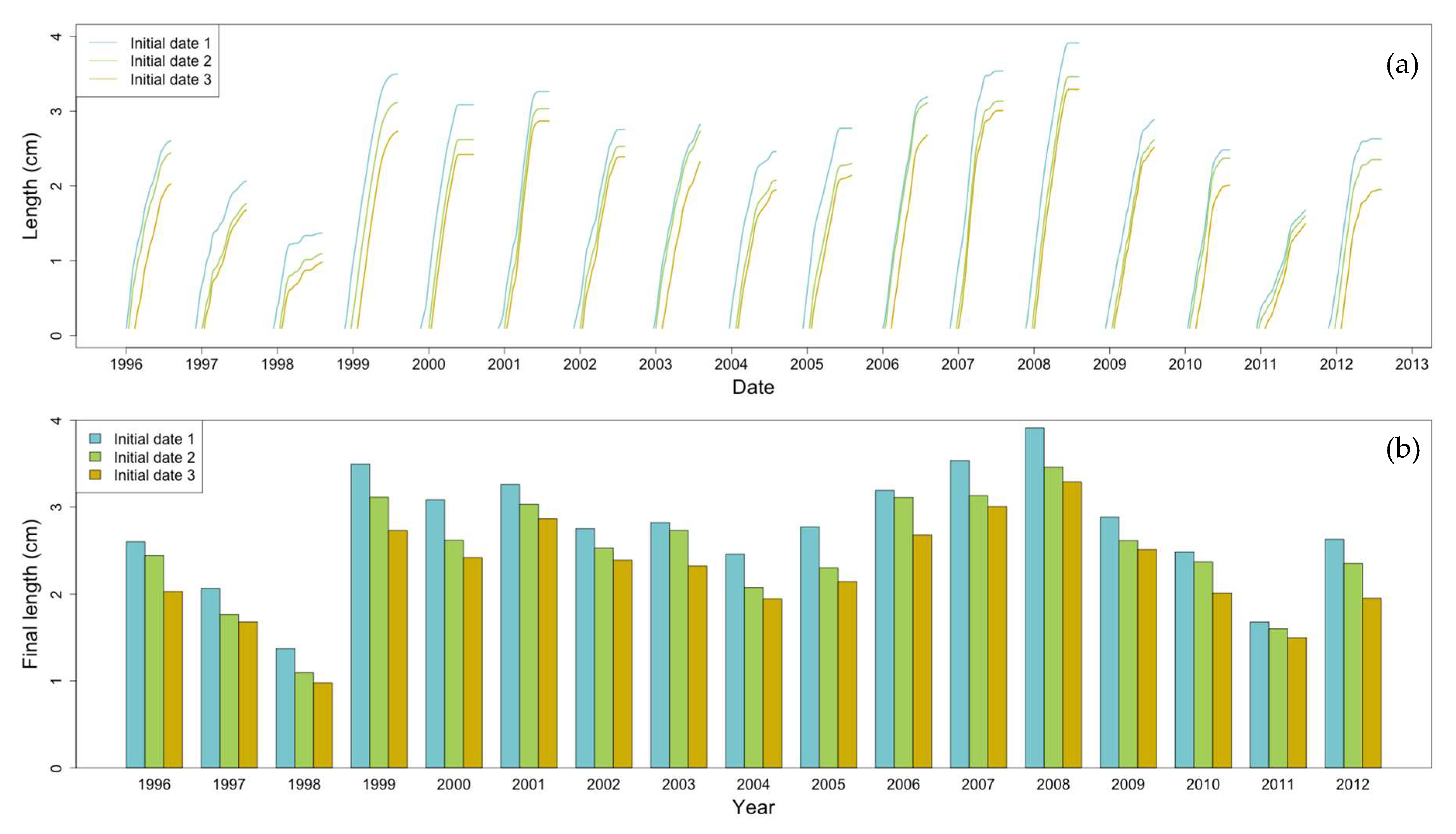
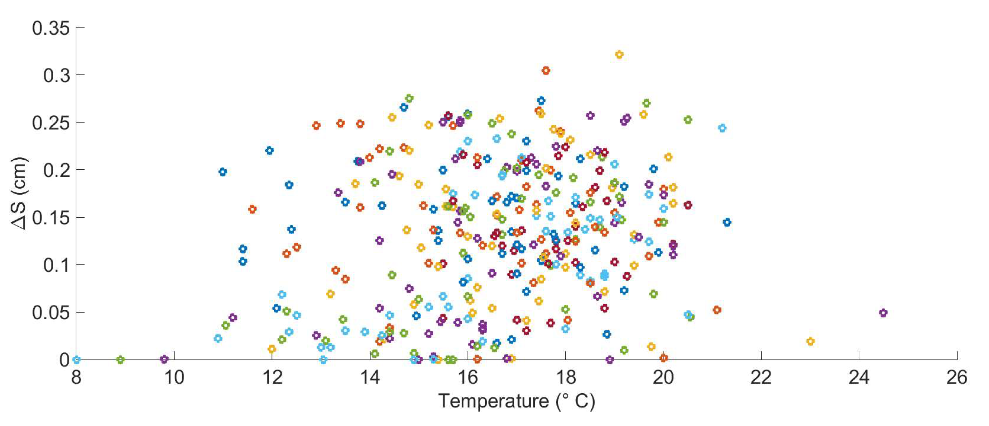
2.6. The Relation between Environmental Factors, Growth, and the Start of Macro-Colonization

The Gamma process simulates increments for each time interval of τ which correspond here to variations in mussel shell length (ΔS_t,τ). The parameterization of the function can integrate the environmental variables. Temperature is a variable of the DEB model, but Chl. a concentration is the main driver of growth. It was therefore decided to parameterize the Gamma process only with Chl. a. However, due to potential coupled effects between temperature and Chl. a, we analyzed the correlation between temperature and growth over the time-series. From ΔS obtained from DEB simulations, the scatter diagram of ΔS vs. temperature showed that there was no significant correlation between these two variables with a Pearson correlation coefficient ρ = 0.21 (Figure 4). That means that temperature is not a key driver of shell growth. On the contrary, there was a structured relationship between growth and Chl. a (Figure 5). It can be noted that uncertainty increases when Chl. a increases. Moreover, there is a ΔS plateau showing that the capability of an individual to grow is limited by the additional food supply: a concentration higher than 8 µg·L⁻¹ does not lead to a larger ΔS. This is due to a well-described physiological phenomenon of maximum somatic growth in bivalves [39,40].

The relationship between the start of macro-colonization and the concentration of Chl. a is presented in Figure A3 in Appendix A. There is no significant correlation between these two variables with a Pearson correlation coefficient ρ = −0.02. This property is of first importance, as it will govern the simulation strategy. Simulation of inception times (start of macro-colonization) requires temperature time-series only, and the modeling of mussel growth will be carried out independently using Chl. a time-series.

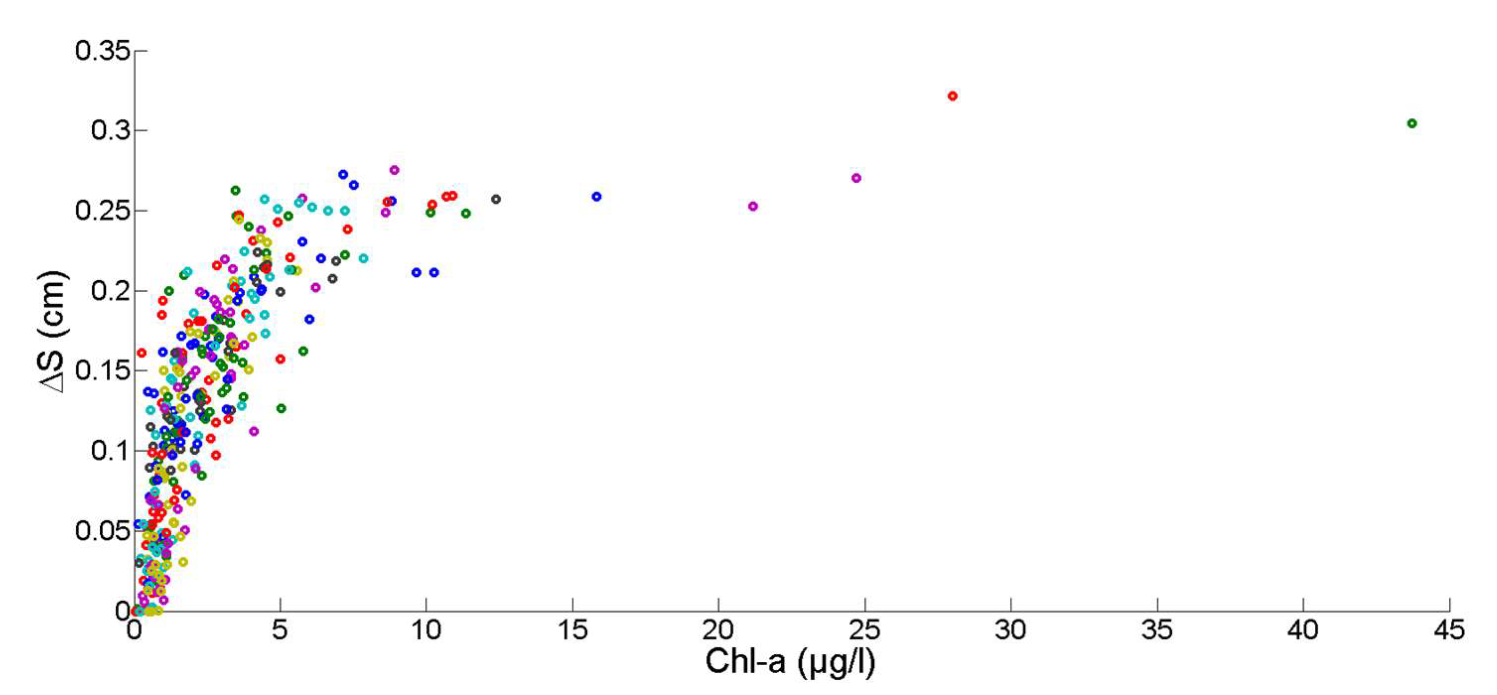
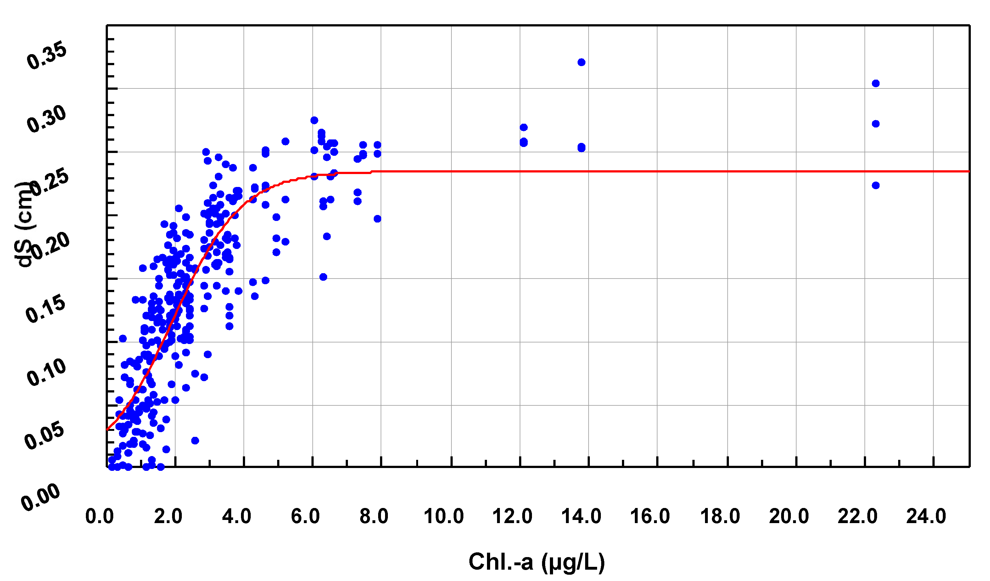
2.7. Chlorophyll Data Aggregation for Growth Computation

In order to improve the biological consistency of our simulations, we tested the possibility to link the individual growth of blue mussels to Chl. a concentration aggregated over a time-step instead of using instantaneous values. The integrated value of Chl. a was simply defined as:

$$C_{(T_{(i)}:T_{(i+n)})}=\frac{1}{n}{\displaystyle \underset{T_{(i)}}{\overset{T_{(i+n)}}{\int }}Chl(t)dt, i=1:36-n}$$

(2)

where C_(.) is the aggregated Chl. a; T_(i), is a 10 day period, and Chl(t), is the linear equation of Chl. a obtained from linear interpolation between adjacent measured values for a colonization period, and n is the number of 10 day time intervals after (i), in which the data aggregation is performed. The best correlation between ΔS and Chl. a has been obtained for a monthly aggregation (3 time intervals, n = 2 in (2)). This time-step preserved the spring bloom typical of the seasonal dynamic of phytoplankton at the study site latitude.

In order to identify the non-linear relationship between growth and Chl. a, the non-linear regression (3) has been fitted with an R² of 0.74 (Figure 6):

$$\Delta S=\frac{0.235}{1+6.94e^{-1.005(Chl.-a)}}$$

(3)

The ratio of (dΔS/dChl. a) ≤2% has been chosen as a criterion for stabilization based on slope variations; this ratio is consistent with the accuracy of the DEB model. A concentration of Chl. a of 8 µg·L⁻¹ was identified as the threshold beyond which ΔS remained constant at 0.235 cm/time interval. The Chl. a time-series was then truncated with the mentioned threshold to significantly improve the convergence of the Gamma process parameterization, without an important degradation of the database. Note that this threshold depends on the metabolism of the organism and is, therefore, species-specific.

2.8. Non-Stationary Modeling of Shell Growth through Stochastic Gamma Process

2.8.1. Growth Approximation through Gamma Processes Meta-Models

Considering the aforementioned characteristics of the mussel’s colonization, and in order to model the temporal dynamic of structure deterioration, a stochastic approach based on Gamma processes has been selected [41]. Since the introduction of the Gamma process in reliability [42], it has been used commonly to model stochastic cumulative and uncertain deterioration phenomena for the maintenance optimization of various industrial systems. Indeed, the Gamma process is an analytically tractable stochastic process accumulating over time in a sequence of positive increments. Recently, it has been widely used to model cumulative degradation processes, such as corrosion, fatigue, crack growth, creep, degrading health, erosion, and wear in engineering systems and structures [11,41,43,44].

The Gamma process is a special case of a non-decreasing jump stochastic process that properly captures the temporal variability associated with the deterioration dynamic. This justified the choice of the non-stationary state-dependent Gamma process. The non-stationary Gamma process is a widely used mathematical model to describe a degradation process whose growth rate at time t depends only on the current state of the parameters and not on the accumulated damage up to t [45]. The complete Gamma process function is defined by two parameters: a shape function α_S and a scale function β_S (4). We discredited time horizon into equal intervals of length τ = 10 days. Then, the state-dependent non-stationary and bivariate Gamma process was represented as a series of state-stationary Gamma processes in each time interval. The rate of the deterioration process can thus be considered as the process resulting from the Gamma process variations from one time-interval to another. The deterioration increment in a given time interval ΔS_t,τ has been considered to be a random variable with a shape function (α_S) dependent of the present deterioration state S_t,τ and a second variable, the state of chlorophyll-a concentration C_t,τ. Thus, for each time step τ, we have:

$$\forall S_{t,\tau }>0:S_{t,\tau },\Delta S_{t,\tau },\tau :\Delta S(\tau ;S_t,C_t):\Gamma ({\alpha }_S(S_t,S_t).\tau ,{\beta }_S)$$

(4)

where S_t,τ is the shell length for each time interval of τ and α_S and β_S are the shape and scale functions of the Gamma process, respectively. To simplify the modeling of this process, it has been assumed that the scale function β_S was constant and Gamma process was only governed by the shape function [11].

2.8.2. Parameter Estimation of the Gamma Process (Learning Phase)

In order to simulate the growth of blue mussel submitted to fluctuations of Chl. a in each time interval τ, the parameters of the developed Gamma process have to be estimated. The deterioration increments have been calculated by the simple subtraction of consecutive individual shell lengths and the resulting database used for deterioration density estimation is denoted as:

$$\left\{\left(C_{t,\tau }^i,S_{t,\tau }^i,\Delta S_{t,\tau }^i\right);t>0, i\in 〚1,N-1〛\right\}$$

(5)

where N is the number of years (in this study N = 17). In order to estimate the parameters of the Gamma process, the Expectation-Maximization (EM) method has been employed. The program starts by scanning the database and indexes the values of C(t) and S(t) time-series; then using the observed data, initial parameters are estimated and used to start an iterative EM algorithm. The Gamma process parameters have been estimated and determined as:

$$\Delta S(\tau ;S_t,C_t):\Gamma \left({\alpha }_S=\left(0.198+1.68C_t\right)\exp \left(\frac{-{\left(S_t-0.44\right)}^2}{6.512}\right),{\beta }_S=0.039\right).$$

(6)

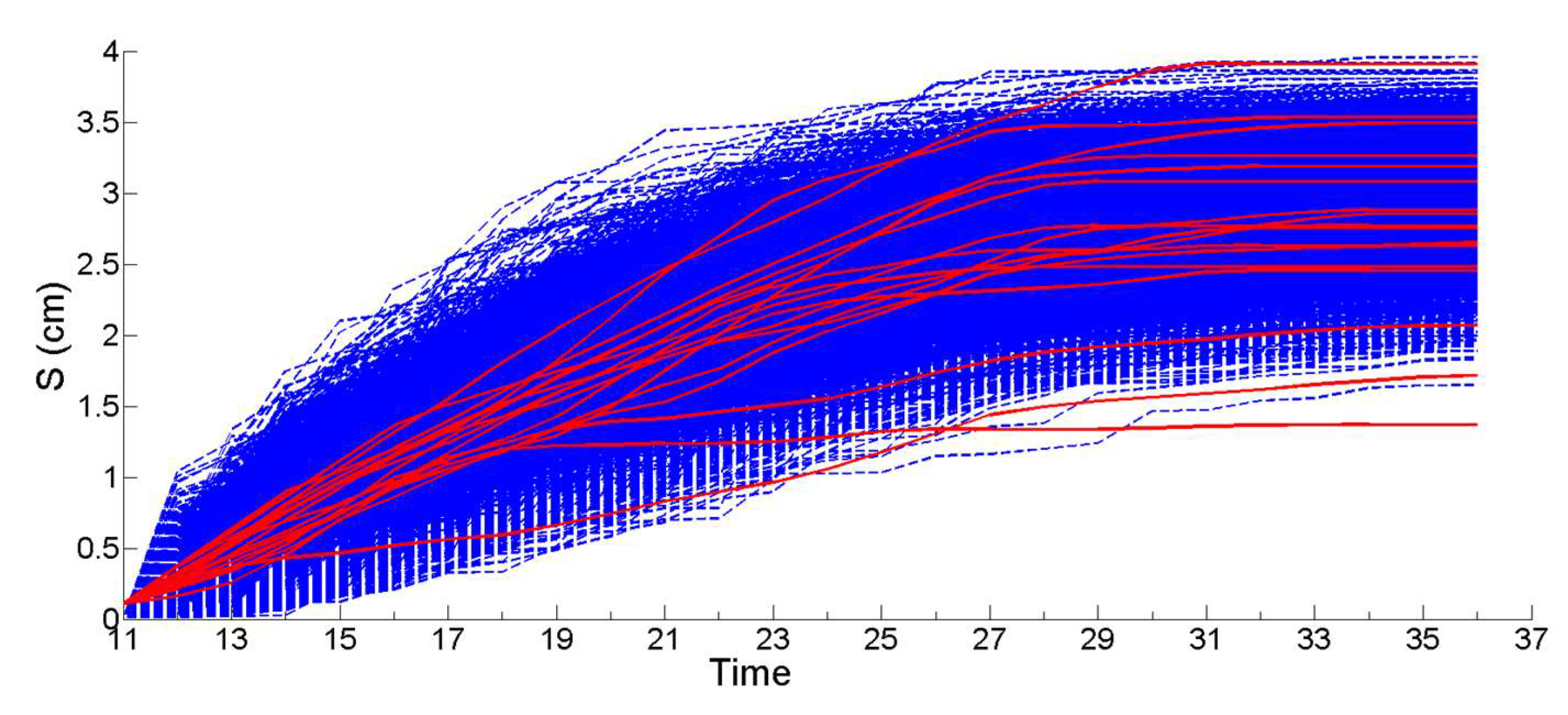
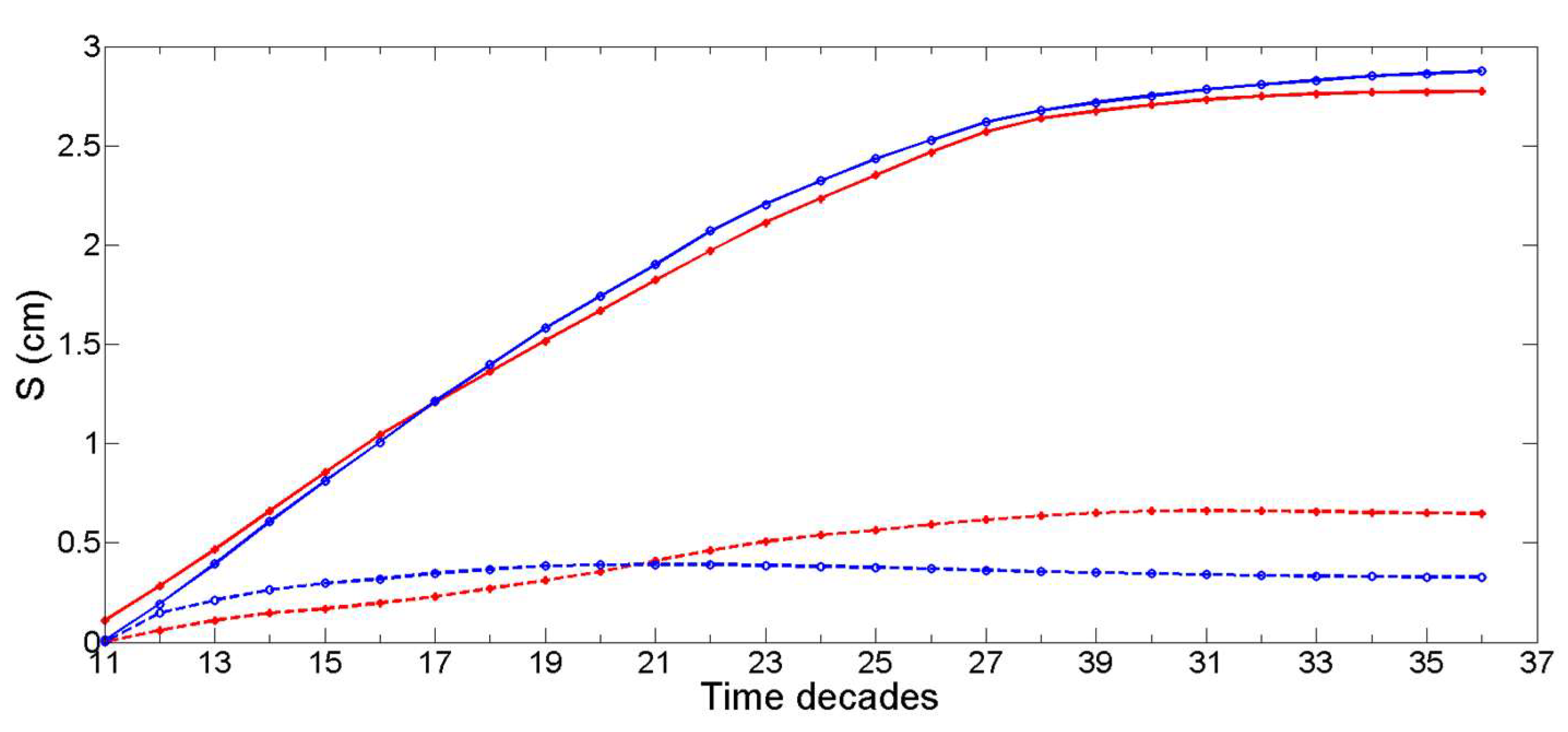
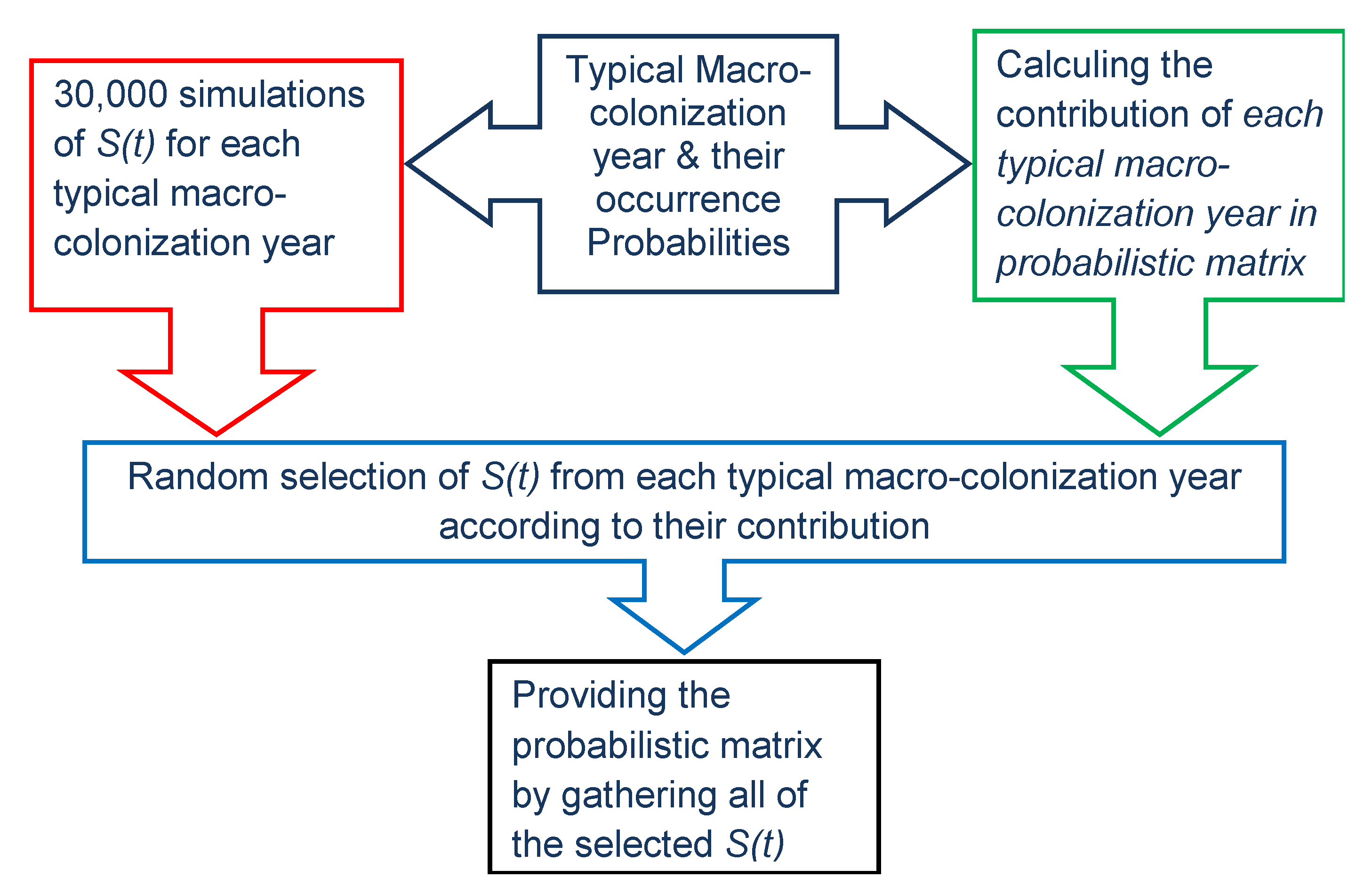
2.8.3. Stochastic Simulation from Gamma Process (Propagation Phase)

Once the Gamma process has been estimated, the DEB data are not needed anymore and we can use the Chl. a database to predict the growth rate of mussels. The macro-colonization can be then simulated with the Gamma process function (6) and consider the Chl. a database for 10 typical macro-colonization years from the 17 year time-series. We considered this database to be representative of the dispersion from a richer database in respect to the frequency of the main phenomena and their consequences. Thus, each environmental input (Chl. a time-series C(t)) is considered with the same weight as the growth uncertainty (biological process). The 5000 simulated growth curves obtained by the Gamma process (50 realizations of C(t) for each of the 10 Chl. a time-series) and individual growth curves simulated with the DEB model are compared in Figure 7. Each growth curve is simulated from one realization of the Gamma process with Chl. a randomly sampled from the 17 year time-series database: uncertainties for Chl. a. and the simulation of S at a given time have herein the same weight in statistical terms. After one year of growth, the mussel shell length time-series S(t) simulated with the Gamma process encompassing the extreme values obtained with the DEB model. Moreover, stabilization is reached (asymptotic behavior) after the 30th time periods when the growth is stabilized at a mature age. At the beginning of the simulations (first 25 weeks), a higher variability was observed with the Gamma process; this would lead to conservative estimations of marine growth characteristics colonizing the structure. From an engineering perspective, it is essential to reach a good representation of the distribution of maximum values of S, which is the case here.

Note that the Gamma process model accounts for the stabilization of shell growth during one or several time steps: that phenomenon is observed in the DEB simulation and actually represents a lack of available food. To complete this statistical analysis, the average and the standard deviation of individual shell length curves are presented in Figure 8. These curves were similar for both methods throughout the simulation period. The Gamma process simulations were a bit conservative in terms of shell length overestimation. The standard deviation curves showed differences between the two approaches. This may be due to the choice of the constant scale parameter β_S, which controls the response dispersion of the Gamma process. Note that there is also a statistical bias when estimating standard deviation from the DEB time-series due to the limited amount of data (17 trajectories).

2.9. Effect of Marine Growth and Hydrodynamic Forces on Jackets

From the structural point of view, marine growth may affect dynamical behavior, resistance to fatigue or extreme loading. We focused here on the latter. Offshore platforms are generally gathered in two families: bottom fixed and floating. Many works studied the effect of marine growth and hydrodynamic forces on components (cylindrical beams) of fixed steel framed offshore structures called jackets for which the component diameter (1 m) is small in comparison with wavelength during storms (100–400 m). This type being, on the one hand, the most popular in oil and gas industry and also for the offshore wind turbines substation, and on the other hand very sensitive to marine growth (fatigue and extreme loading). The analysis of marine growth effect on hydrodynamic forces could be categorized into two groups as follows:

(i)

experimental modeling of hydrodynamic forces for cylinders with different roughness conditions [46,47]. Recent studies are mostly concentrated on the water particle velocity and acceleration measurement techniques.

(ii)

evaluation of hydrodynamic forces by the physical modeling of marine growth characteristics obtained from in-situ measurements [6,48]. These studies were based on inspections carried out during survey campaigns. They advocate guidelines for the probabilistic modeling of hydrodynamic forces at a given time. The biofouling database has been analyzed to propose a model of marine growth evolution and to update the design criterion. A physical response surface matrix has been proposed in order to provide a probabilistic modeling of the environmental loading on jacket type offshore structures. The key parameter is the increase of the structural diameter due to the marine growth thickness.

In the present study, we are considering the non-linear effect of the roughness of marine growth on the loading during a yearly growth. The results from laboratory studies focused mainly (i) on the regular shape of marine growth and homogeneous colonization around the cylinder and (ii) on mean thickness. Moreover, for time computation constraints (stochastic simulations of wave and marine growth) and because it allows explicitly introducing the role of marine growth, we used Morison modeling [49] for which the link between homogeneous roughness and loading is available. Because roughness is non-homogeneous and random, an uncertainty was added.

2.9.1. Effect of Marine Growth on Morison’s Equation

Usually, Morison’s model [49] is used to estimate hydrodynamic forces on tubular offshore structures like jackets, using the particle kinematics obtained from the wave heights and periods. It should be noted that for the jacket structures Morison’s equation is valid because the structural diameters (D) are small compared to wavelengths λ (D/λ < 0.2). This equation can be employed from medium to deep-water depth [49]. It has been shown to be very appropriate for an expansion in the stochastic domain [48]. This equation is denoted as:

$$F_{Morison}=F_D+F_I=\frac{1}{2}\rho C_{D}Du\left|u\right|+C_M\frac{\rho \pi D^2}{4}\dot{u}$$

(7)

where F_Morison is the hydrodynamic force per unit length of the member (N/m), F_D is the drag force per unit length of the member (N/m), F_I is inertia force per unit length of the member (N/m), C_D is the drag coefficient, C_M is inertia coefficient, ρ is the density of water, D is member diameter (m), and u is velocity of wave’s water particles (m/s), $\dot{u}$ is the acceleration of wave’s water particles (m/s²). u and $\dot{u}$ are computed by Stoke’s model [50] from the knowledge of metocean data: wave height H and period T.

Generally, the inertia term of the mentioned equation becomes important for small waves or for members with large diameters [48], otherwise the drag term will be dominant. Marine growth increases the surface roughness and hence changes both the drag and inertia forces. The variations induced by the presence of marine growth impress the hydrodynamic forces in a non-linear way.

Considering the effect of biofouling on hydrodynamic coefficients in Morison’s equation, some researchers have proposed a model for the drag coefficient as a linear regression function of the thickness and roughness [51,52]. According to the recommended practice of [3], an additional parameter that affects the drag coefficient of elements with circular cross-sections is the relative roughness, e = k/D_e. The surface Roughness k is the average peak-to-valley height of hard growth organisms and the effective member diameter De can be obtained as:

$$D_e=D_c+2 Th$$

(8)

where D_c is the outer diameter of the clean member and Th is the biocolonization thickness (i.e., the mean of distributed thickness around the diameter) obtained by circumferential measurements [3]. API [3] gives the relationship between De and the steady-flow drag coefficient (C_DS) (9).

$$C_{DS}=a+\frac{b}{\raisebox{1ex}{$k$}\!\left/ \!\raisebox{-1ex}{$De$}\right.+c}; a=0.07152, b=-2.9\times {10}^{-4}, c=4.12\times {10}^{-4}.$$

(9)

C_D is then computed from the knowledge of C_DS and the Keulegan-Carpenter number KC_mg according to [3,6].

This approach allows measuring the influence of roughness on the drag coefficient and therefore the drag force as well as their evolution with time. This leads us to choose an uncertainty model for the relationship between the size of the shell and the roughness in Morison’s equation.

Coefficients of fluid-structure interactions are modeled from the knowledge of the hydraulic flow regime around the structural components [47]. Reynolds R_e and Keulegan-Carpenter KC numbers are essential for characterizing the flow regime [6]. For most offshore jacket structures in extreme conditions, Reynolds numbers are put into the post-critical flow regime, where the steady-flow drag coefficient C_DS for circular cylinders is independent of Reynolds number [3,53].

2.9.2. Stochastic Modeling of Marine Growth and Hydrodynamic Parameters

There is not enough knowledge, nor enough observations, about the settlement of blue mussels on offshore structures and a 100% cover was considered on the component. In order to account for the diameter of the colonized structural member, the marine growth thickness time-series Th(t) should be modeled. Marine growth thickness is modeled as a Gamma process Th_t,τ deduced from the simulated individual shell length time-series S_t,τ for blue mussels in each time interval. For simplicity at this step of modeling, it has been assumed that the individual shell length time-series S(t) gives the average size time-series Th_t,τ with a multiplying uncertain factor (10): it follows a uniform distribution with support [0.3; 0.6] at each of the i 10 day periods.

$$Th(t)=\left\{\left(T{h}_1,\dots ,T{h}_n\right); 0.3 S_i\le T{h}_i\le 0.6 S_i, i\in 〚1,37〛\right\}.$$

(10)

This uncertainty accounts for the geometrical arrangement of the shells (Figure 9).

For roughness, on the one hand, there is a lack of on-site measurements and on the other, the available relationship between roughness and hydrodynamic forces (9) relies on a uniform roughness around the component [3]. Hence, roughness is also modeled as a Gamma process k_t,τ based on individual shell length time-series S_t,τ (11), with a random factor following a uniform distribution with support [0.2; 1]. The latter is a model error for modeling the uncertainty when quantifying the real effect of a randomly distributed roughness around the component. Note that intensive developments on underwater image processing are emerging [54,55,56], enabling one to envisage progress in on-site measurements. Recent works investigate the relationship between non-homogenous roughness and loading [57,58]. The wide range of uncertainty will, therefore, decrease in the next decade. Consequently, the error of computation of equivalent roughness is significant and the interval in (11) is large: it includes the stochastic distribution of shells around a tubular component and the error of model for computing the equivalent roughness.

Finally, the time-series of surface roughness k(t) and marine growth average thickness Th(t) have been considered independently as the random value uniformly distributed in an interval bounded to a ratio of individual shell length S(t):

$$k(t)=\left\{\left(k_1,\dots ,k_n\right); 0.2 S_n\le k_n\le S_n, n\in 〚1,37〛\right\}.$$

(11)

The relative surface roughness e(t) time-series are deduced (e(t) = k(t)/De(t)) and C_DS(t) time-series have been simulated according to (9).

This study deals with two major time variant random variables in the hydrodynamic calculations, the meteocean data including a couple of wave height and period (H, T) and the stochastic process generating the individual shell length S_t,τ in each time interval τ from (4). Parameters of Gamma processes Th_t,τ, and k_t,τ are dependent of individual shell length St,τ and the hydraulic parameters (Re_mg, KC_mg), and therefore drag coefficients C_D, depend on individual shell length S_t,τ and the couple of wave height and period (H, T).

Thus, parameters of Th_t,τ affect the hydrodynamic coefficients through the relationships between the hydraulic parameters (R_e, KC) and the diameter of the elements, which is dependent of the coefficient of Th_t,τ itself [6]. The next section will explain how these cross-effects are accounted for.

2.9.3. The Stochastic Modeling Wave Loading in the Presence of Marine Growth

Figure 10 summarizes the steps of drag forces computation in a flowchart. It should be noted that the steps of hydrodynamic coefficients calculation are based on an interpolation of experimental curves [6] presented by [3].

The main steps of this flowchart are detailed below ((#X) means the step in circle X in the figure):

• (#1) Statistical Identification: the employed parameters are the heights of extreme waves H and associated periods T. They are modeled with a random variable, whose probability is conditioned by the wave direction θ;
• (#2) A kinematic model for the fluid for computation of water particle velocity: the Stokes model [50] is used. It assumes that the fluid is Newtonian and irrotational and the trajectory of the fluid particles is elliptical. The kinematics field deduced from the velocity potential can be defined at any point M of coordinates x and z. The maximum velocity u_m (#5) is deduced and is used in the computation of KC and Re (#6).
• (#3) The fluid-structure Interaction model: this level is involved in the hydrodynamic coefficients determined by using the recommendation of [3].
• For the probabilistic modeling of CD, in order to avoid multiplying the case studies, only vertical elements under the wave crest are analyzed. This implies high horizontal speeds and accelerations that generate very small forces, which means that the inertia forces in (7) are very low and will be neglected in the following.
• (#4) The colonized diameter D_e(t) is a stochastic process that results from the increase Th(t) of the initial radius of the clean component. Starting from (8), the diameter is computed by multiplying D_c by the factor θ_mg. The latter is computed from the thickness Th(t) (12):

  $$D_e=D_c+2 \overline{th}={\theta }_{mg} D_c \mathrm{with} {\theta }_{mg}=\left(1+\frac{2 T{h}_{t,\tau }}{D_c}\right).$$

  (12)

Random or stochastic nature of variables or processes is reminded at the beginning of the flowchart by writing as a function of the hazard ω.

According to API RP 2A WSD [3] and DNV-RP-C20 [4], since the flow regime is post-critical (R_e > 5 × 105) by using 100 year-return wave characteristics, the drag coefficient does not depend on R_e but rather on KC_mg and C_DS. Note that API ([3], section C2.3.1b7, p. 143 and p. 145) provides, in fact, a piecewise model on two intervals depending on KC or KC/C_DS and the scales of these models are different. It results in two effects on the evolution of the drag force (C_D): first for some values of C_DS it is the cause of discontinuity of the model at KC = 12 and second, it is very difficult to analyze directly the effect of C_DS. This is visible in Section 3.2.

Extreme wave characteristics (H, T) of the Gulf of Guinea have been considered for the hydrodynamic calculation, which is a specific site with low KC_mg values. Moreover, it gathers wave and wind-sea values and the spectrum is very similar to the one in French Atlantic offshore sites. Using meteocean data from this region allowed us to cover a large range of KC_mg to better illustrate the non-linear effects of marine growth on the drag coefficient evolution and hence on the load probabilistic distribution. This covers almost all configurations of Atlantic French offshore sites. Joint distribution of the extreme height and period for a return period of 100 years for the Gulf of Guinea are simulated based on [7]. It has been provided by recombination of sea states from the knowledge of the H-T scatter diagram. Representation of the joint distribution for wave height and the 100 year return period is presented in [59]. Note that breaking waves are not considered here.

We focused on drag forces acting on vertical cylindrical components under the wave crest with a diameter of 0.762 m (corresponding to the diameter of a Φ30″ leg). Note that, for simplicity, the probability of storm occurrence is independent of time and can happen in every 10 day periods of the macro-colonization period. This assumption is conservative. The time-series of surface roughness k(t) and marine growth thickness Th(t) obtained from the individual shell length time-series S(t) have been considered for the determination of the C_DS (C_D in steady flow) time-series (C_DS(t) = f(kt,τ/D_e). In this paper, knowing C_DS, a numerical fitting of the curve of C_D = f(KC_mg) given in [3] is used and is plotted in Section 3.2 (lower multi-linear curve for the smooth cylinder).

3. Results

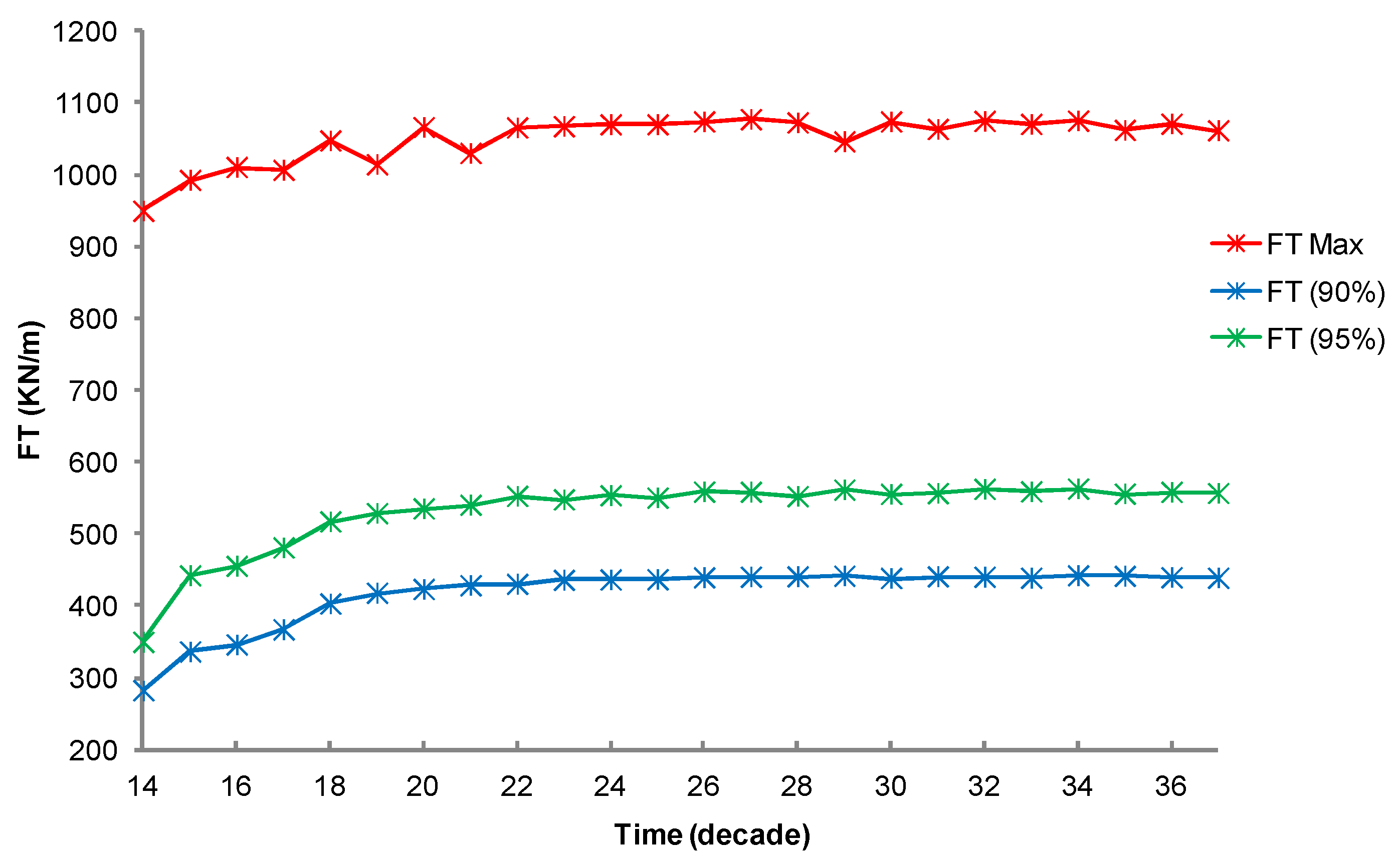
3.1. Simulation of the Drag Force Evolution from the Stochastic Time-Series of blue Mussels

This section aims to assess the evolution of the drag coefficient (CD) by mixing all of the typical macro-colonization time-series according to their occurrence probabilities by considering the macro-colonization inception times in the initiation phase (Section 2.2, Section 2.3 and Section 2.4). The individual shell length time-series for all the typical macro-colonization years are necessary to provide the probabilistic matrix of individual shell length. This matrix consists of the individual shell length time-series for all typical macro-colonization years, which are weighted by the occurrence probability of each typical macro-colonization year. Therefore, 30,000 simulations (10,000 simulations for each macro-colonization inception time in one year) have been performed to provide the individual shell length of blue mussels for each typical macro-colonization year.

The individual shell length time-series S(t) of the blue mussels are simulated from the developed Gamma process (Section 2.8) from the inception times for typical macro-colonization years. No correlation between macro-colonization inception time conditioned by the temperature and the aggregate Chl. a (Ct) levels are observed (Section 2.6). Therefore, the levels are simulated independently. Hence, all the time-series of aggregate C(t) could be used for the simulation of the individual shell length time-series S(t)) for each typical macro-colonization year.

The individual shell length time-series simulation procedure is as follows: the typical macro-colonization year determined by the temperature is first selected. Then, the individual shell length time-series S(t) are simulated from the Gamma process. This simulation is performed according to the aggregated Chl. a time-series, which have been selected randomly, generating one S(t) from one C(t). Thus, we obtain the same statistical weight for the inception and growth by choosing an aggregated Chl. a time-series randomly for each simulation.

Figure 11 illustrates the estimated individual shell length time-series for the 2nd typical macro-colonization (starting dates at 11, 14, and 17 10 day periods) and 200 simulations, as an example. The highest jumps are observed for the 18th to 22nd 10 day periods, because of the important peak occurrence in the aggregated Chl. a time-series in 2001, 2007, and 2008 (see Figure 12).

The simulation allows the individual shell length matrix to represent all of the typical macro-colonization years. The contribution of the individual shell length time-series could be obtained as:

$$N_t=N_S\times P_t$$

(13)

where, N_t is the numbers of time-series for the typical macro-colonization year of S(t), which should be selected randomly, N_s is the sample size (here equal to 30,000), and P_t is the occurrence probability of the typical macro-colonization year (Table 2). The simulation procedure is illustrated in Figure 13. The KC, C_D, and drag forces are then computed according to the flowchart reported in Figure 10.

3.2. Statistical Analysis of the Transfer of Distributions

Quality of distribution transfer or uncertainty propagation is a well-known criterion for the analysis of the change of the distribution (its parameters or probabilistic law), especially for matrix response surfaces [48]. We focus first on the evolution of shell length distribution. Figure 14 illustrates the three most interesting 10 day periods representing insignificant (the 11th 10 day period), intermediate (the 18th 10 day period), and extreme (the 37th 10 day period) roughness values. The distribution of shell length changes from bimodal (the 11th and 18th 10 day periods) to normal (the 37th 10 day period), depending on time. It should be noted that the shape of the shell length distribution evolves strongly with time, which will lead to significant variations in the distribution of C_D along with its support due to the dependence of C_DS to k/D_e in (9). The mixing of sources of uncertainties due to independent macro-colonization inception time and independent growth builds finally a normal distribution as expected from the Central Limit Theorem.

Figure 15 illustrates the distributions of drag coefficients C_D as a function of KC for the three above-mentioned 10 day periods. First, we plot the bounds of the relationship (CD)–(KC) with lower and upper lines that depict, respectively, the smooth and roughened cylinders’ drag coefficients. The discontinuity comes from the discontinuity of curves in the standards generated by the various scales (CD/CDS, CD, KC, KC/CDS) used around KC = 12. Note that this discontinuity for the smooth and roughed cylinders follows, respectively, a potential positive and a negative jump of the C_D. Second, the scatter plots are reported in red, moving from the lower part to the upper part from 11th to 37th decade 10 day periods. Consequently, the distribution of C_D is affected. An important point is that the distribution maintains two modes, the uppermost being around 1.2 and the lowermost following the shift of the non-linear transfer function, from 0.2 to 0.6 (see the 37th 10 day period). It demonstrates the evolution of the drag coefficients C_D for the individual shell length from the non-linear transfer of the distribution of KC and during the probabilistic macro-colonization year (from the 11th to the 37th 10 day period). Finally, the probability of the highest values (typically 1.8) increases with time, which is a key result because it will potentially affect the distribution tail of the corresponding loading and decrease structural reliability. There is not a clear distinction between the macro-colonization inception times because of the mixing of all typical macro-colonization years. Indeed, the mixing of a large amount of potential macro-colonization inception times does not allow one to distinguish between the contribution of each year in terms of the mode in the distribution.

4. Discussion

Previous results give the opportunity for discussing the effect of our modeling on post-treated results, such as wave loading in the presence of marine growth. We now compare the distribution of D_e and C_DS (Figure 16). The distributions of D_e are mono-modal because of the combination of all typical macro-colonization years. The distributions of C_DS are bimodal and become mono-modal from the smooth to the ultra-roughened condition at the end of the macro-colonization period.

Distribution of the drag force F_T is plotted on the same Figure 16 to better illustrate differences in distribution (mode and tails) and the transfer of these distributions. The drag force is exponentially distributed. The right distribution tail moves to higher values according to time, thereby decreasing the reliability. We analyze this distribution tail after the computation of F_{T_MAX} (note that distributions are bounded) and the fractiles F_T(90%), F_T(95%). Figure 17 shows the evolution of these statistics after each 10 day period. The latter increase smoothly with time except for the increase during one month and a half (from 10 day period 11 to 18). Finally, there is a great difference between the extreme values (F_{T_MAX}) and the fractiles (F_T(90%) and F_T(95%), confirming a long distribution tail that was observed already in Figure 16.

5. Conclusions

The originality of this work lies in the choice to consider biocolonization as a cumulative deterioration phenomenon and to simulate trajectories relying on individuals’ characteristics through a state-dependent model to compute the probabilistic distribution of loading. The latter is a key input for structural reliability. As far as the authors know, this is the first time that bio-colonization has been considered as consecutive stochastic jumps governed by a gamma process. The developed non-stationary, state-dependent Gamma process was selected as a flexible and simple to perform methodology, which was used to generate an individual shell length time-series for blue mussels. Results of the simulation reveal that the method can capture the distribution and especially the extreme values of the observed shell length. The macro-colonization inception times determined in the initiation phase may be considered as one of the criteria for the installation or cleaning time of the structures through the maintenance programs strategy. One of its advantages is that it can be extended to other organisms, such as oysters, with the possibility of adding or modifying the parameters that influence individual growth and shape.

A model was used to investigate the drag coefficient evolution exerted by extreme waves during the mussel’s growth. Three types of uncertainties have thus been considered:

-

Environmental: due both to the physics of waves (height, period) and water parameters (temperature and chlorophyll-a).

-

Modeling: with an uncertainty of modeling from the shell size to the thickness and the roughness in the sense of API regulation.

-

Biological: accounting for the inter-individual variability.

-

Moreover, calculation of hydrodynamic forces due to the biocolonization using meteo-ocean data as well as biological data is a complex task and generates two types of difficulties.

-

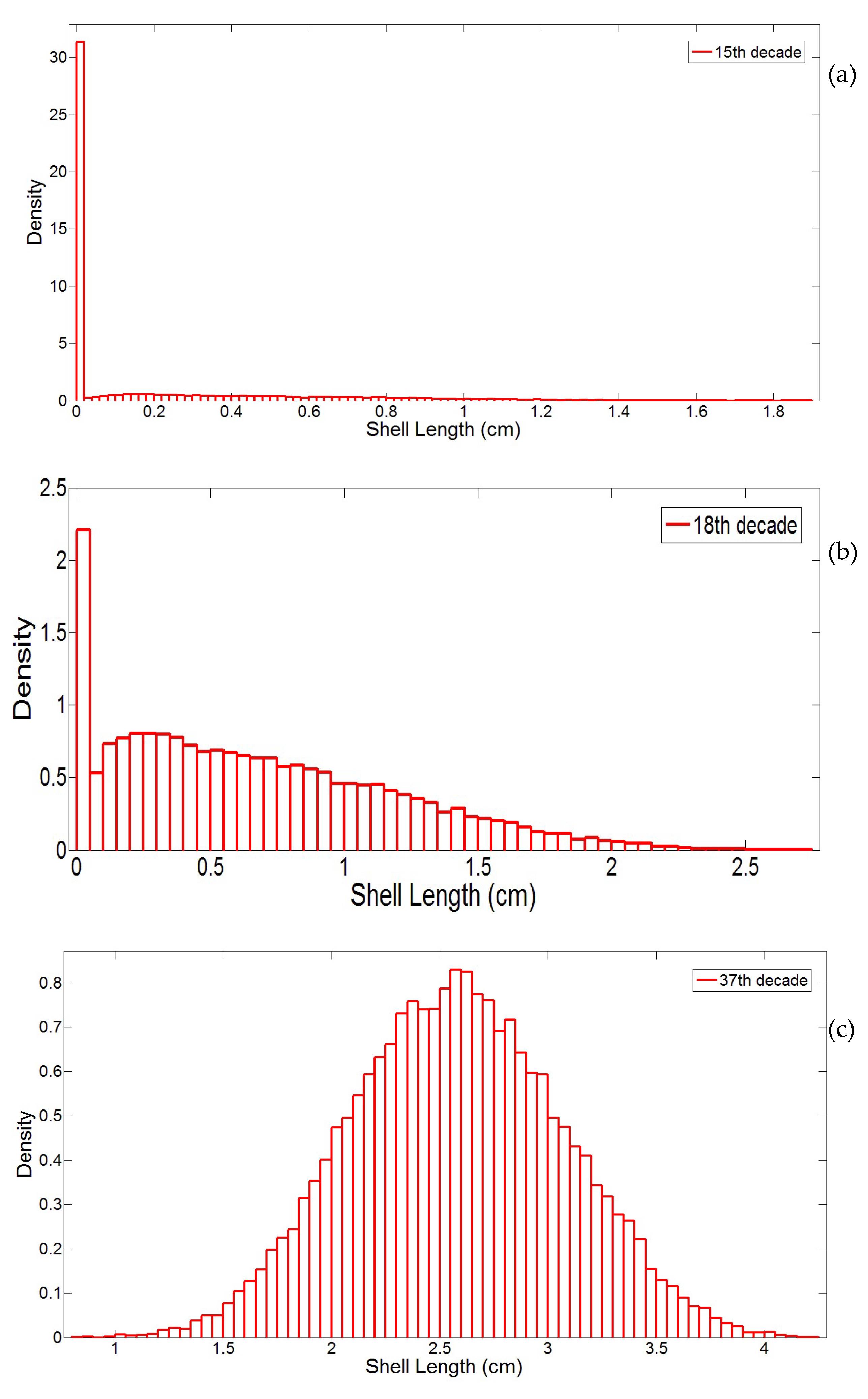
First, the distribution of input variables that can be multi-modal (e.g., individual shell length) due to the various macro-colonization inception times.

-

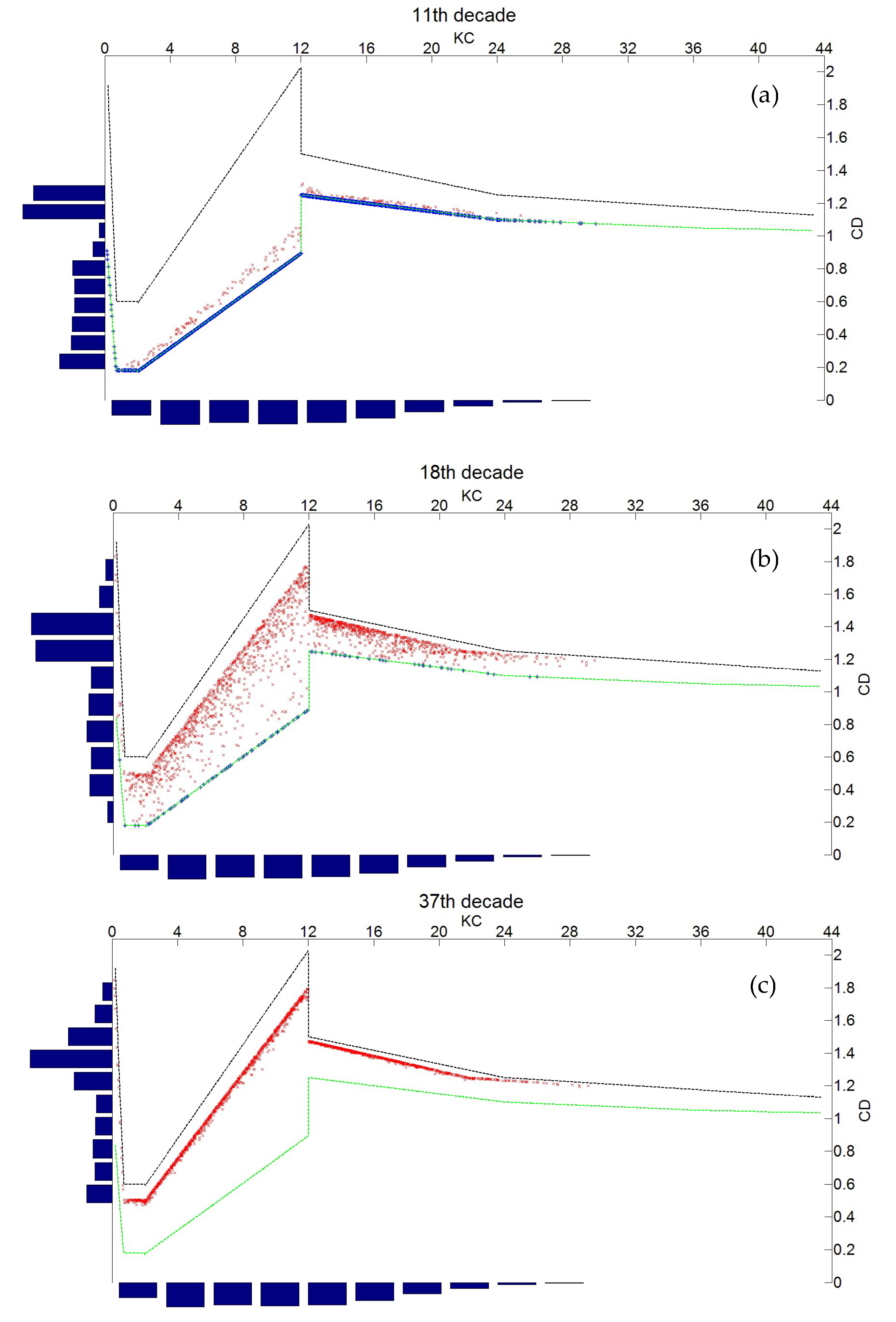
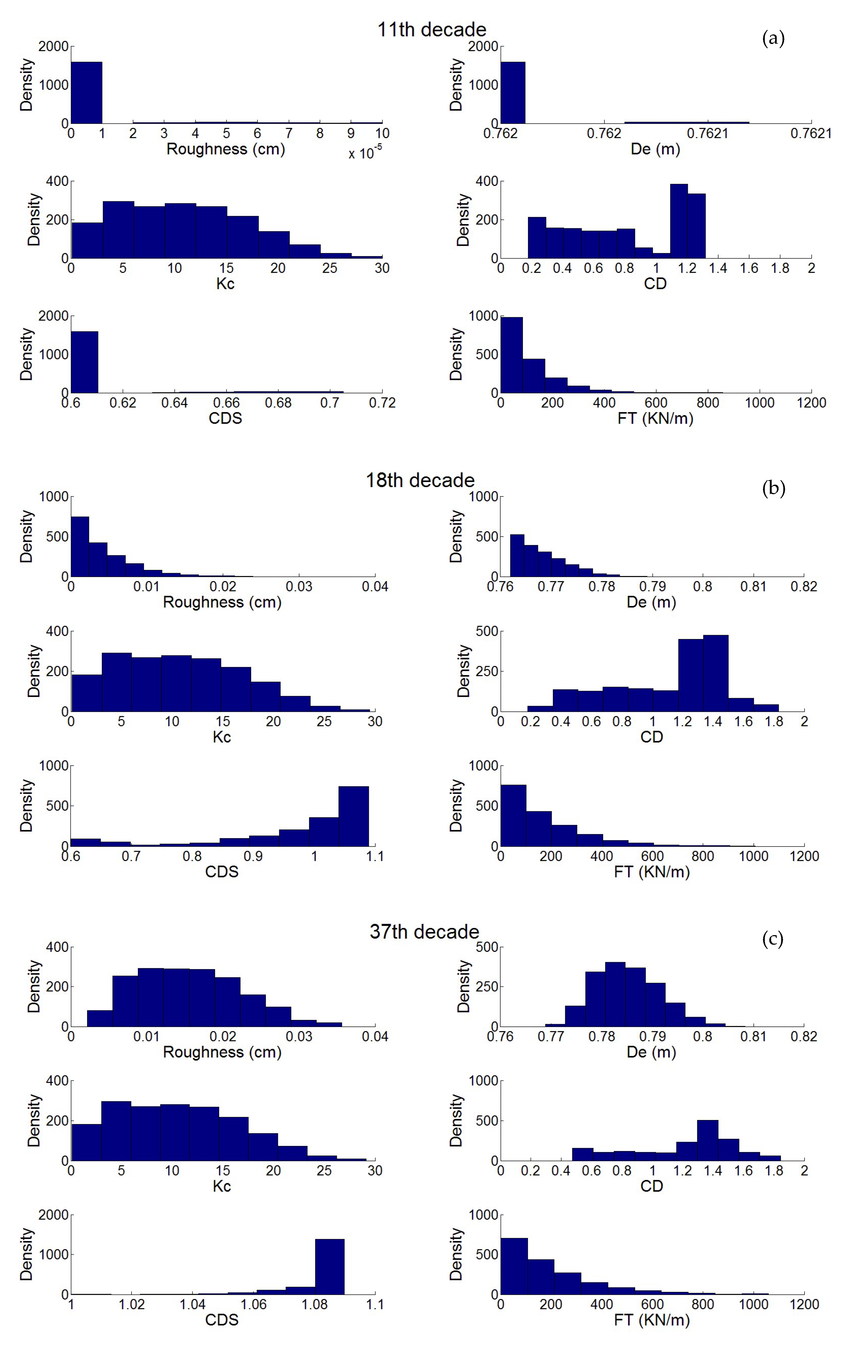
Second, the nonlinear transfer from the Keulegan Carpenter number to drag coefficient generates bimodal distributions from mono-modal ones.

A full probabilistic simulation that allows predicting the evolution of drag forces in a reliability context has been developed. The evolution of physical parameters due to individual growth has been presented in a time-series form. Using the empirical curves recommended by API standards to obtain wake amplification factors in a probabilistic context resulted in an abnormal discontinuity when passing the critical value KC = 12. Thus, these curves may not perfectly explain the evolution of the drag coefficient in a probabilistic context.

This study highlights the site-specific property of biofouling and, therefore, constructs a condition-based methodology for the modeling of biocolonization. Considering the site-specific property of biofouling, it is not logical to define a similar strategy for the maintenance and periodical cleaning programs of offshore structures without consideration of the specifications of each site. Therefore, periodical monitoring campaigns could be very useful in understanding the reaction of biofouling to environmental parameters, especially after installation or cleaning programs, and to establish the adequate maintenance strategy for each site. It allows the model to be updated as well and hence increases prediction accuracy. For some structures, it may not be necessary to clean all members completely to allow a macro-fouling community to develop and create artificial reefs that would be useful for fisheries and biodiversity. Some limitations discussed in the paper highlight that further research is requested:

-

A single species was studied in a place where we can find barnacles and even algae. For the latter, relationships for the computation of drag coefficients are less developed and research is required.

-

There is uncertainty in the definition of roughness and its use by engineers, which is the reason why an uncertainty of modeling is added in this paper. Recent works [60] have proposed some improvements, but this is still an open area of study. Quantification from on site inspections is possible [54], thereby opening a new area for more representative tests in laboratories.

-

The probability of the occurrence of storms depends on seasons and could be introduced to reduce the conservatism.

-

Effects of the Cd variations on dynamics should be introduced to expand the method to fatigue assessment.

-

In the same manner, inertia forces and current could be added to get a more global influence of marine growth.

This work can be extended to floating structures once the correlation between thickness and weight is known.

6. Patents

A patent was developed in view to measure on site the marine growth and update the model: Schoefs F., Ameryoun H. (2013) «Biocolmar: Offshore Station for Measuring and Collecting Data in an Underwater Environment», 21 October 2013, N° 1360256.

References

1. Heaf, N.J. The Effect of Marine Growth on The Performance of Fixed Offshore Platforms in The North Sea. In Proceedings of the Offshore Technology Conference, Houston, TX, USA, 30 April–3 May 1979; p. 14. [Google Scholar] [CrossRef]
2. Jusoh, I.; Wolfram, J. Effects of marine growth and hydrodynamic loading on offshore structures. J. Mek. 1996, 1, 77–98. [Google Scholar]
3. API RP 2A WSD. Recommended Practice for Planning, Designing, and Constructing Fixed Offshore Platforms, 21st ed.; American Petroleum Institute: Washington, DC, USA, 2005; Volume 2. [Google Scholar]
4. DNV. Recommended Practice Det Norske Veritas; DNV-RP-C20; DNV: Oslo, Norway, 2010. [Google Scholar]
5. Faber, M.H.; Hansen, P.F.; Jepsen, F.D.; Moller, H.H. Reliability-Based Management of Marine Fouling. J. Offshore Mech. Arct. Eng. 2001, 123, 76. [Google Scholar] [CrossRef]
6. Schoefs, F.; Boukinda, M.L. Sensitivity Approach for Modeling Stochastic Field of Keulegan–Carpenter and Reynolds Numbers Through a Matrix Response Surface. J. Offshore Mech. Arct. Eng. 2010, 132, 011602. [Google Scholar] [CrossRef]
7. Boukinda, M.L. Surface de Réponse des Efforts de Houle des Structures Jackets Colonisées par des Bio-salissures. Ph.D. Thesis, Université de Nantes, Nantes, France, 2007. [Google Scholar]
8. Schoefs, F.; Boukinda, M.L. Modelling of Marine Growth Effect on Offshore Structures Loading Using Kinematics Field of Water Particle. In Proceedings of the Fourteenth International Offshore and Polar Engineering Conference, Toulon, France, 23–28 May 2004; pp. 419–427. [Google Scholar]
9. Joschko, T.J.; Buck, B.H.; Gutow, L.; Schröder, A. Colonization of an artificial hard substrate by Mytilus edulis in the German Bight. Mar. Biol. Res. 2008, 4, 350–360. [Google Scholar] [CrossRef]
10. Maar, M.; Bolding, K.; Petersen, J.K.; Hansen, J.L.S.; Timmermann, K. Local effects of blue mussels around turbine foundations in an ecosystem model of Nysted off-shore wind farm, Denmark. J. Sea Res. 2009, 62, 159–174. [Google Scholar] [CrossRef]
11. El Hajj, B.; Schoefs, F.; Castanier, B.; Yeung, T. A condition-based deterioration model for the stochastic dependency of corrosion rate and crack propagation in a submerged concrete structure. Comput. Aided Civ. Infrastruct. Eng. 2014, 32, 18–33. [Google Scholar] [CrossRef]
12. Ameryoun, H. Probabilistic Modeling of Wave Actions on Jacket Type Offshore Wind Turbines in Presence of Marine Growth. Ph.D. Thesis, Université de Nantes, Nantes, France, 2015. [Google Scholar]
13. Koojiman, S. Dynamic Energy and Mass Budgets in Biological Systems; Cambridge University Press: Cambridge, UK, 2000. [Google Scholar]
14. Koojiman, S. Dynamic Energy Budget Theory for Metabolic Organization. Cambridge University Press: Cambridge, UK, 2010. [Google Scholar]
15. Dürr, S.; Thomason, J. Biofouling; Wiley-Blackwell: New York, NY, USA, 2009; Available online: http://eu.wiley.com/WileyCDA/WileyTitle/productCd-1405169265.html (accessed on 18 December 2009).
16. Railkin, A.I. Marine Biofouling: Colonization Processes and Defenses; CRC Press: Boca Raton, FL, USA, 2003. [Google Scholar]
17. Liu, Y. Modeling the Time-to-Corrosion Cracking of the Cover Concrete in Chloride Contaminated Reinforced Concrete Structures. Ph.D. Thesis, Virginia Polytechnic Institute and State University, Blacksburg, VA, USA, 1996. [Google Scholar]
18. Newell, R.I.E. Species Profiles: Life Histories and Environmental Requirements of Coastal Fishes and Invertebrates (North and Mid-Atlantic); Biological Report, 82(11.102) TR EL-82-4 June; US dept of Interior/US Army Corps of Engineers: Baltimore, MD, USA, 1989. [Google Scholar]
19. Bruijs, M.C.M. Biological Fouling Survey of Marine Fouling on Turbine Support Structures of the Offshore Windfarm Egmond aan Zee. Report Prepared for Noordzeewind; 50863511-TOS/PCW 10-4207, OWEZ_R_112_T1_20100226; KEMA Nederland, B.V.: Arnhem, The Netherlands, 2010. [Google Scholar]
20. Langhamer, O.; Wilhelmsson, D.; Engström, J. Artificial reef effect and fouling impacts on offshore wave power foundations and buoys—A pilot study. Estuarine. Coast. Shelf Sci. 2009, 82, 426–432. [Google Scholar] [CrossRef]
21. Gosling, E. Bivalve Molluscs: Biology, Ecology and Culture; Wiley-Blackwel: Hoboken, NJ, USA, 2003. [Google Scholar]
22. Barillé Boyer, A.-L. Contribution à l’étude des potentialités conchylicoles du Pertuis Breton. Ph.D. Thesis, Université d’Aix-Marseille II, Marseille, France, 1996. [Google Scholar]
23. Garen, P.; Robert, S.; Bougrier, S. Comparison of growth of mussel, Mytilus edulis, on longline, pole and bottom culture sites in the Pertuis Breton, France. Aquaculture 2004, 232, 511–524. [Google Scholar] [CrossRef]
24. Rosland, R.; Strand, Ø.; Alunno-bruscia, M.; Bacher, C.; Strohmeier, T. Applying Dynamic Energy Budget (DEB) theory to simulate growth and bio-energetics of blue mussels under low seston conditions. J. Sea Res. 2009, 62, 49–61. [Google Scholar] [CrossRef] [Green Version]
25. Widdows, J. Physiological ecology of mussel larvae. Aquaculture 1991, 94, 147–163. [Google Scholar] [CrossRef]
26. Dutertre, M.; Beninger, P.G.; Barillé, L.; Papin, M.; Rosa, P.; Barillé, A.-L.; Haure, J. Temperature and seston quantity and quality effects on field reproduction of farmed oysters, Crassostrea gigas, in Bourgneuf Bay, France. Aquat. Living Resour. 2009, 22, 319–329. [Google Scholar] [CrossRef]
27. Bayne, B.L. Growth and the delay of metamorphosis of the larvae of Mytilus edulis (L.). Ophelia 1965, 2, 1–47. [Google Scholar] [CrossRef]
28. Bayne, B.L.; Worrall, C.M. Growth and Production of Mussels Mytilus edulis from Two Populations. Mar. Ecol. 1980, 3, 317–328. [Google Scholar] [CrossRef]
29. Van Harden, R.; Koojiman, S. Application of a Dynamic Energy Budget Model to Mytilus edulis (L.). Neth. J. Sea Res. 1993, 31, 119–133. [Google Scholar] [CrossRef]
30. Page, H.M.; Hubbard, D.M. Temporal and spatial patterns of growth in mussels Mytihs edulis on an offshore platform: Relationships to water temperature and food availability. Exp. Mar. Biol. Ecol. 1987, 111, 159–179. [Google Scholar] [CrossRef]
31. Thomas, Y.; Mazurié, J.; Alunno-Bruscia, M.; Bacher, C.; Bouget, J.-F.; Gohin, F.; Pouvreau, S.; Struski, C. Modelling spatio-temporal variability of Mytilus edulis (L.) growth by forcing a dynamic energy budget model with satellite-derived environmental data. J. Sea Res. 2011, 66, 308–317. [Google Scholar] [CrossRef]
32. Thompson, R. Production, reproductive effort, reproductive value and reproductive cost in a population of the blue mussel Mytilus edulis from a subarctic environment. Mar. Ecol. Prog. Ser. 1984, 16, 249–257. [Google Scholar] [CrossRef]
33. REPHY dataset. French Observation and Monitoring program for Phytoplankton and Hydrology in coastal waters. 1987–2016. Metrop. Data 2017. [Google Scholar] [CrossRef]
34. Hernandez-Farinas, T.; Soudant, D.; Barille, L.; Belin, C.; Lefebvre, A.; Bacher, C. Temporal changes in the phytoplankton community along the French coast of the eastern English Channel and the southern Bight of the North Sea. Mar. Sci. 2013, 70, 1439–1450. [Google Scholar] [CrossRef]
35. Barillé, L.; Lerouxel, A.; Dutertre, M.; Haure, J.; Barillé, A.L.; Pouvreau, S.; Alunno-Bruscia, M. Growth of the Pacific oyster (Crassostrea gigas) in a high-turbidity environment: Comparison of model simulations based on scope for growth and dynamic energy budgets. J. Sea Res. 2011, 66, 392–402. [Google Scholar] [CrossRef] [Green Version]
36. Handå, A.; Alver, M.; Edvardsen, C.V.; Halstensen, S.; Olsen, A.J.; Øie, G.; Reinertsen, H. Growth of farmed blue mussels (Mytilus edulis L.) in a Norwegian coastal area; comparison of food proxies by DEB modeling. J. Sea Res. 2011, 66, 297–307. [Google Scholar]
37. Pouvreau, S.; Bourles, Y.; Lefebvre, S.; Gangnery, A.; Alunno-Bruscia, M. Application of a dynamic energy budget model to the Pacific oyster, Crassostrea gigas, reared under various environmental conditions. J. Sea Res. 2006, 56, 156–167. [Google Scholar] [CrossRef] [Green Version]
38. Ren, J.S.; Ross, A.H. Environmental influence on mussel growth: A dynamic energy budget model and its application to the greenshell mussel Perna canaliculus. Ecol. Model. 2005, 189, 347–362. [Google Scholar] [CrossRef]
39. Barillé, L.; Prou, J.; Héral, M.; Razet, D. Effects of high natural seston concentrations on the feeding, selection, and absorption of the oyster Crassostrea gigas (Thunberg). J. Exp. Mar. Biol. Ecol. 1997, 212, 149–172. [Google Scholar] [CrossRef]
40. Bayne, B.L.; Newell, R.C. Physiological energetics of marine molluscs. Mollusca 1983, 4, 407–515. [Google Scholar]
41. Van Noortwijk, J.M. A survey of the application of gamma processes in maintenance. Reliab. Eng. Syst. Saf. 2009, 94, 2–21. [Google Scholar] [CrossRef]
42. Abdel-Hameed, M. A Gamma Wear Process. IEEE Trans. Reliab. 1975, R-24, 152–153. [Google Scholar] [CrossRef]
43. Cheng, T.; Pandey, M.D.; Van Der Weide, J.A.M. The probability distribution of maintenance cost of a system affected by the gamma process of degradation: Finite time solution. Reliab. Eng. Syst. Saf. 2012, 108, 65–76. [Google Scholar] [CrossRef]
44. Van Noortwijk, J.M.; Van der Weide, J.A.M.; Kallen, M.J.; Pandey, M.D. Gamma processes and peaks-over-threshold distributions for time-dependent reliability. Reliab. Eng. Syst. Saf. 2007, 92, 1651–1658. [Google Scholar] [CrossRef]
45. Guida, M.; Postiglione, F.; Pulcini, G. A time-discrete extended gamma process for time-dependent degradation phenomena. Reliab. Eng. Syst. Saf. 2012, 105, 73–79. [Google Scholar] [CrossRef]
46. Sarpkaya, T. On the Effect of Roughness on Cylinders. J. Offshore Mech. Arct. Eng. 1990, 112, 334. [Google Scholar] [CrossRef]
47. Theophanatos, A. Marine Growth and the Hydrodynamic Loading of Offshore Structures. Ph.D. Thesis, University of Srathclyde, Glasgow, UK, 1988. [Google Scholar]
48. Schoefs, F. Sensitivity approach for modelling the environmental loading of marine structures through a matrix response surface. Reliab. Eng. Syst. Saf. 2008, 93, 1004–1017. [Google Scholar] [CrossRef] [Green Version]
49. Morison, J.R.; Johnson, J.W.; Schaaf, S.A. The Force Exerted by Surface Waves on Piles. J. Pet. Technol. 1950, 2, 149–154. [Google Scholar] [CrossRef]
50. Stokes, G.G. On the theory of oscillatory waves. Trans. Camb. Phil. Soc. 1847, 8, 441–455. [Google Scholar]
51. Wolfram, J.; Jusoh, I.; Sell, D. Uncertainty in the Estimation of Fluid Loading Due to the Effects of Marine Growth, Safety and Reliability Symposium. In Proceedings of the 12th International Conference on Offshore Mechanics and Arctic Engineering (O.M.A.E’93), Glasgow, Scotland, UK, 20–24 June 1993; Volume II, pp. 219–228. [Google Scholar]
52. Kasahara, Y.; Koterayama, W.; Shimazaki, K. Wave Forces Acting on Rough Circular Cylinders at High Reynolds Numbers. In Proceedings of the Offshore Technology Conference, Houston, TX, USA, 6–9 May 2013; p. 12. [Google Scholar] [CrossRef]
53. Troesch, A.W.; Kim, S.K. Hydrodynamic forces acting on cylinders oscillating at small amplitudes. J. Fluids Struct. 1991, 5, 113–126. [Google Scholar] [CrossRef] [Green Version]
54. O’Byrne, M.; Schoefs, F.; Pakrashi, V.; Ghosh, B. An underwater lighting and turbidity image repository for analysing the performance of image based non-destructive techniques. Struct. Infrastruct. Eng. 2018, 14, 104–123. [Google Scholar] [CrossRef]
55. O’Byrne, M.; Schoefs, F.; Pakrashi, V.; Ghosh, B. A Stereo-Matching Technique for Recovering 3D Information from Underwater Inspection Imagery. Comput. Aided Civ. Infrastruct. Eng. 2018, 33, 193–208. [Google Scholar] [CrossRef]
56. O’Byrne, M.; Pakrashi, V.; Schoefs, F.; Ghosh, B. Semantic Segmentation of Underwater Imagery Using Deep Networks. J. Mar. Sci. Eng. 2018, 6, 93. [Google Scholar] [CrossRef]
57. Zeinoddini, M.; Bakhtiari, A.; Schoefs, F.; Zandi, A.P. Towards an Understanding of the Marine Fouling Effects on VIV of Circular Cylinders: Partial Coverage Issue. Biofouling 2017, 33, 268–280. [Google Scholar] [CrossRef]
58. Bakhtiari, A.; Schoefs, F.; Ameryoun, H. Unified Approach for Estimating of The Drag Coefficient In Offshore Structures In Presence Of Bio-Colonization. In Proceedings of the 37th International Conference on Offshore Mechanics and Arctic Engineering (O.M.A.E’18), Madrid, Spain, 17–22 June 2018; p. 78757. [Google Scholar]
59. Nerzic, R.; Prevosto, M.; Frelin, C.; Quiniou, V. Joint Distributions for Wind/waves/current in West Africa and derivation of Multi Variate Extreme I-FORM Contours. In Proceedings of the 17th International Offshore and Polar Engineering Conference, Lisbon, Portugal, 1–6 July 2007; pp. 81–88. [Google Scholar]
60. Schoefs, F.; Bakhtiari, A.; Hameryoun, H.; Quillien, N.; Damblans, G.; Reynaud, M.; Berhault, C.; O’Byrne, M. Assessing and modeling the thickness and roughness of marine growth for load computation on mooring lines. In Proceedings of the Floating Offshore Wind Turbine Conference (FOWT 2019), Montpellier, France, 24–26 April 2019. [Google Scholar]
Figure 1. Schematic diagram of bio-colonization phases and their influencing parameters.
Jmse 07 00158 g001
Figure 2. Inter-annual variations (1996–2012) of water temperature (°C) (a), and chlorophyll-a (Chl. a, µg·L−1) (b), at Le Croisic sampling station (Loire-Atlantique, France). Data from Ifremer/Quadrige/Rephy©.
Jmse 07 00158 g002
Figure 3. (a) Individual annual shell length trajectories simulated by a mussel Dynamic Energy Budget (DEB) model and (b) corresponding final length.
Jmse 07 00158 g003
Figure 4. Scatter diagram of the variations of mussel shell length (ΔS) vs. temperature for 10 days periods during the 17 year time series (each color represents a year of the 1996–2012 time-series).
Jmse 07 00158 g004
Figure 5. Scatter diagram of the variations of mussel shell length (ΔS) vs. Chlorophyll a for 10 days periods during the 17 year time series (each color represents a year of the 1996–2012 time-series).
Jmse 07 00158 g005
Figure 6. Identification of the Chl. a threshold beyond which growth saturation is observed.
Jmse 07 00158 g006
Figure 7. Individual growth trajectories obtained with the DEB model for each year of the 17 year time series (solid red lines) compared with simulated individual growth obtained with the Gamma process approach (dotted blue lines). The time unit represents 10 day periods.
Jmse 07 00158 g007
Figure 8. Comparison of average (solid lines) and standard deviation (dashed lines) of shell length from Gamma process (blue lines) and DEB model (red lines). Time unit represents 10 day periods.
Jmse 07 00158 g008
Figure 9. From biological reality to mechanical abstraction.
Jmse 07 00158 g009
Figure 10. Schematic flowchart of drag force calculation.
Jmse 07 00158 g010
Figure 11. Simulated individual shell length of blue mussels for the 2nd typical macro-colonization (11-12-17). 200 simulations are presented.
Jmse 07 00158 g011
Figure 12. The aggregated Chl. a time-series for the years 2001, 2007 and 2008.
Jmse 07 00158 g012
Figure 13. Schematic procedure of probabilistic individual shell length time-series from the typical macro-colonization year.
Jmse 07 00158 g013
Figure 14. Evolution of shell length distribution as a function of time for three selected 10 day periods: (a) 15th, (b) 18th, (c) 37th.
Jmse 07 00158 g014
Figure 15. Distributions of the drag coefficients (CD) as a function of (KC) values for three selected 10 day periods and Monte-Carlo simulations (cloud of red points): (a) 11th, (b) 18th, (c) 37th.
Jmse 07 00158 g015
Figure 16. Comparison of the distribution of hydrodynamic parameters for the selected 10 day periods: (a) 11th, (b) 18th, (c) 37th.
Jmse 07 00158 g016
Figure 17. Evolution of FTmax, and 90%, 95% fractiles with time.
Jmse 07 00158 g017