Improved Double-Layer Soil Consolidation Theory and Its Application in Marine Soft Soil Engineering


Abstract
:1. Introduction
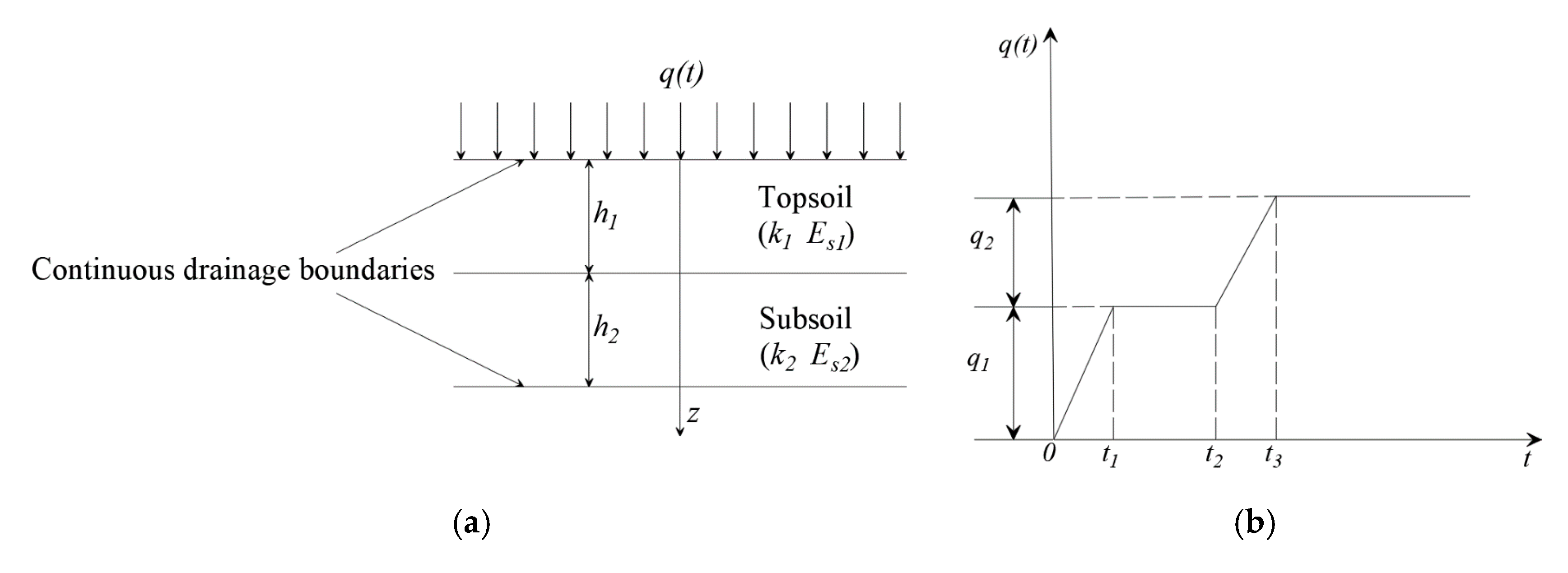
2. Improved Double-Layer Soil Consolidation Theory Considering Continuous Drainage Boundary Conditions
- (1)
- The soil layer is homogeneous and fully saturated.
- (2)
- Soil particles and water are incompressible.
- (3)
- Water seepage and compression of the soil layer occur only in one direction (vertical).
- (4)
- The seepage of water obeys Darcy’s law.
- (5)
- In the osmotic consolidation, the permeability coefficient and the compression coefficient of the soil are constants.
- (6)
- The external load is applied at two levels of average speed.
- (7)
- Additional stress of soil does not decrease with depth under the large area load of highway roadbed.
3. Improved Double-Layer Consolidation Theory Model Verification Analysis
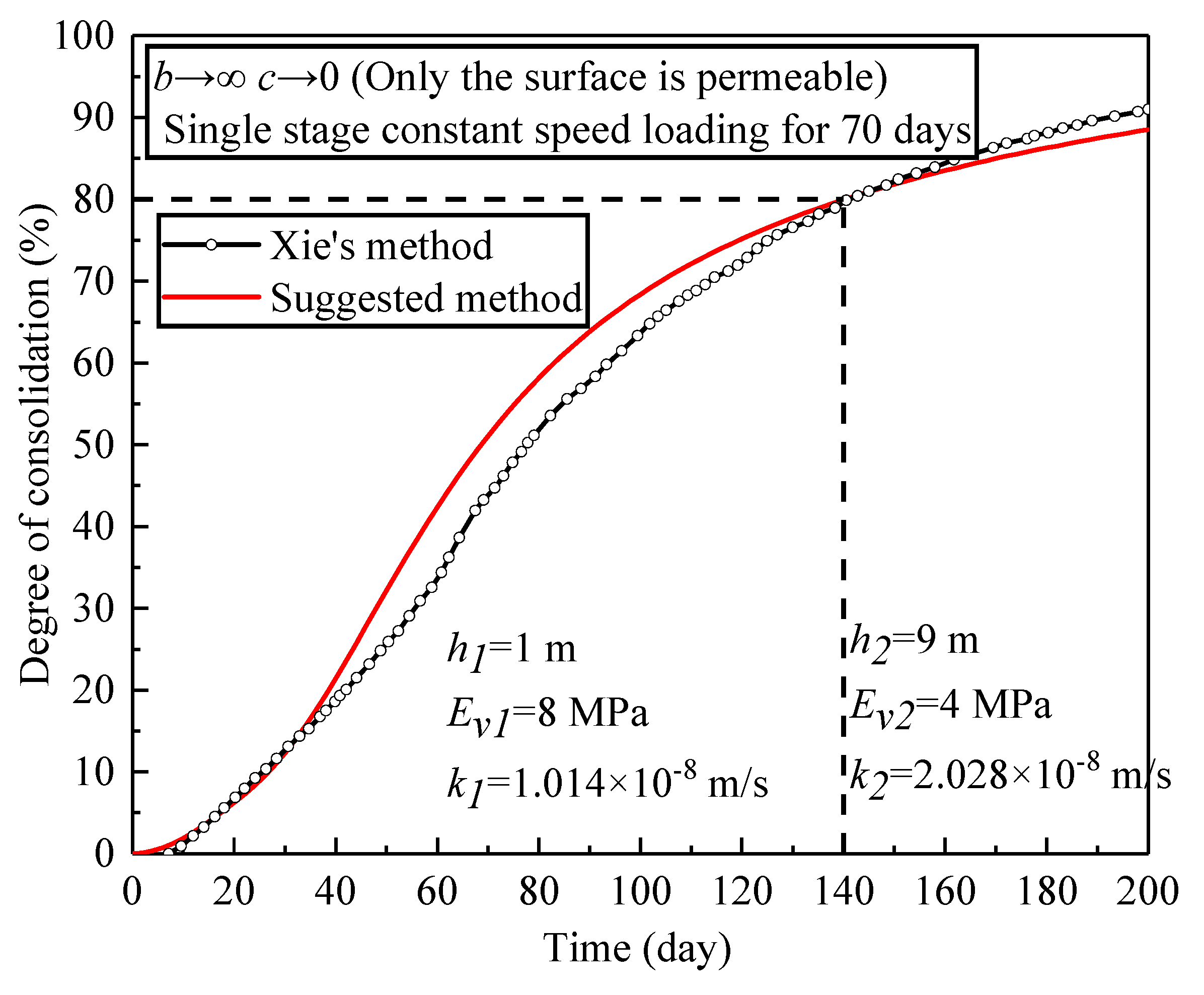
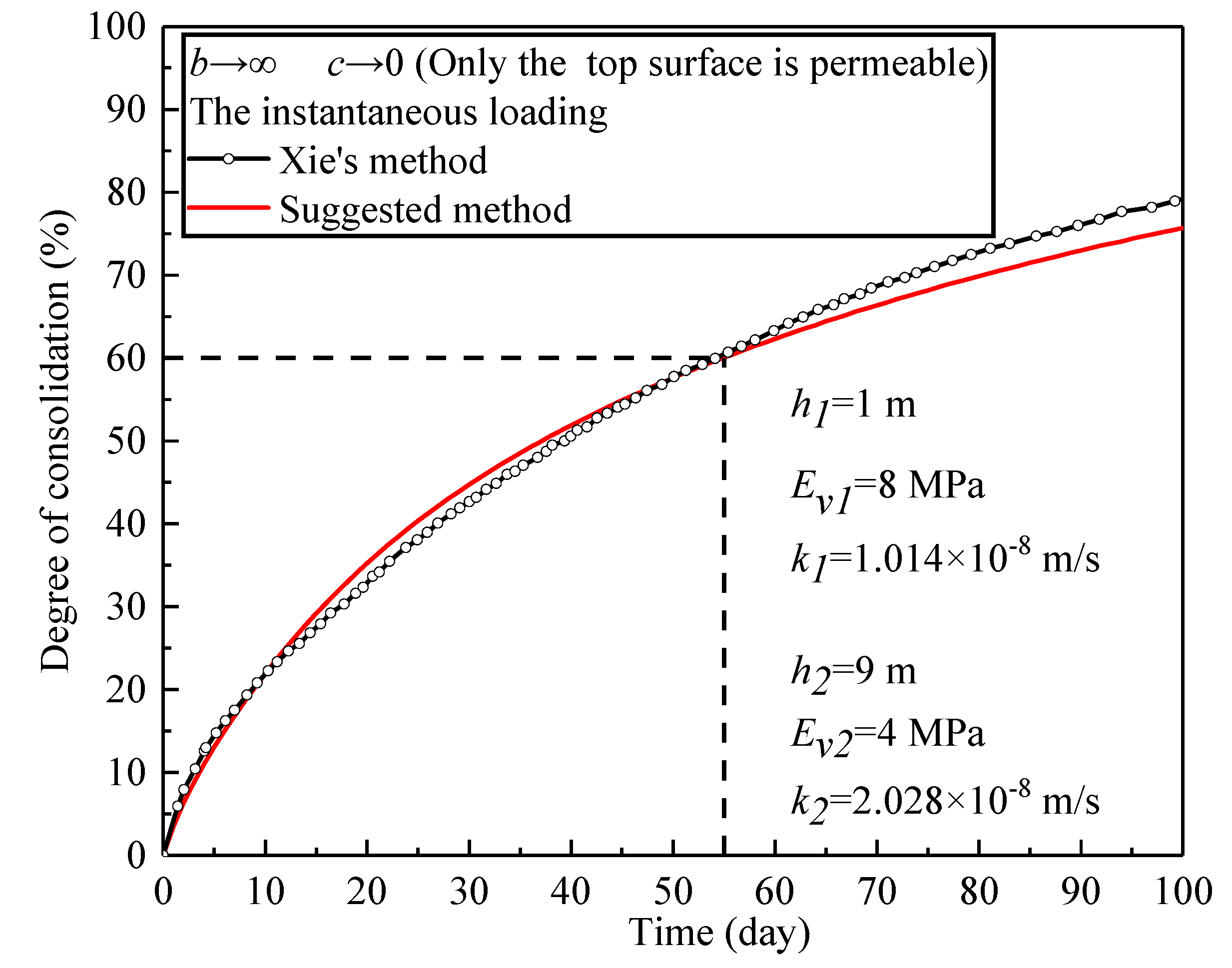
3.1. Degradation Analysis of Perfectly Permeable Boundary Conditions by the Improved Model
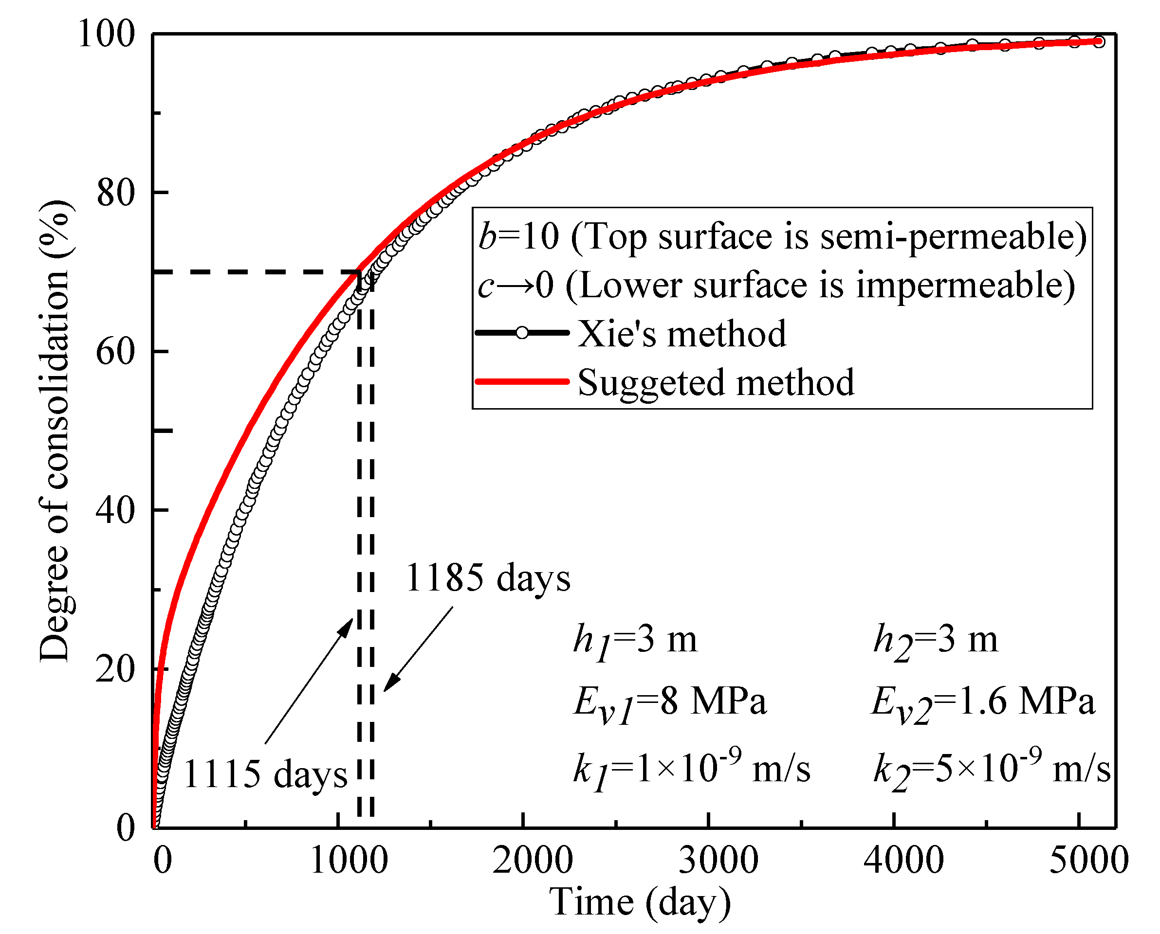
3.2. Degradation Analysis of Semi-Permeable Boundary Conditions by the Improved Model
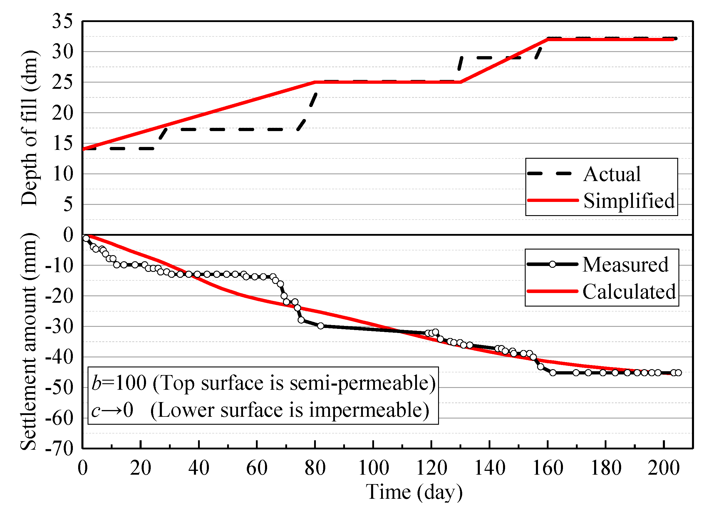
4. Engineering Case Analysis
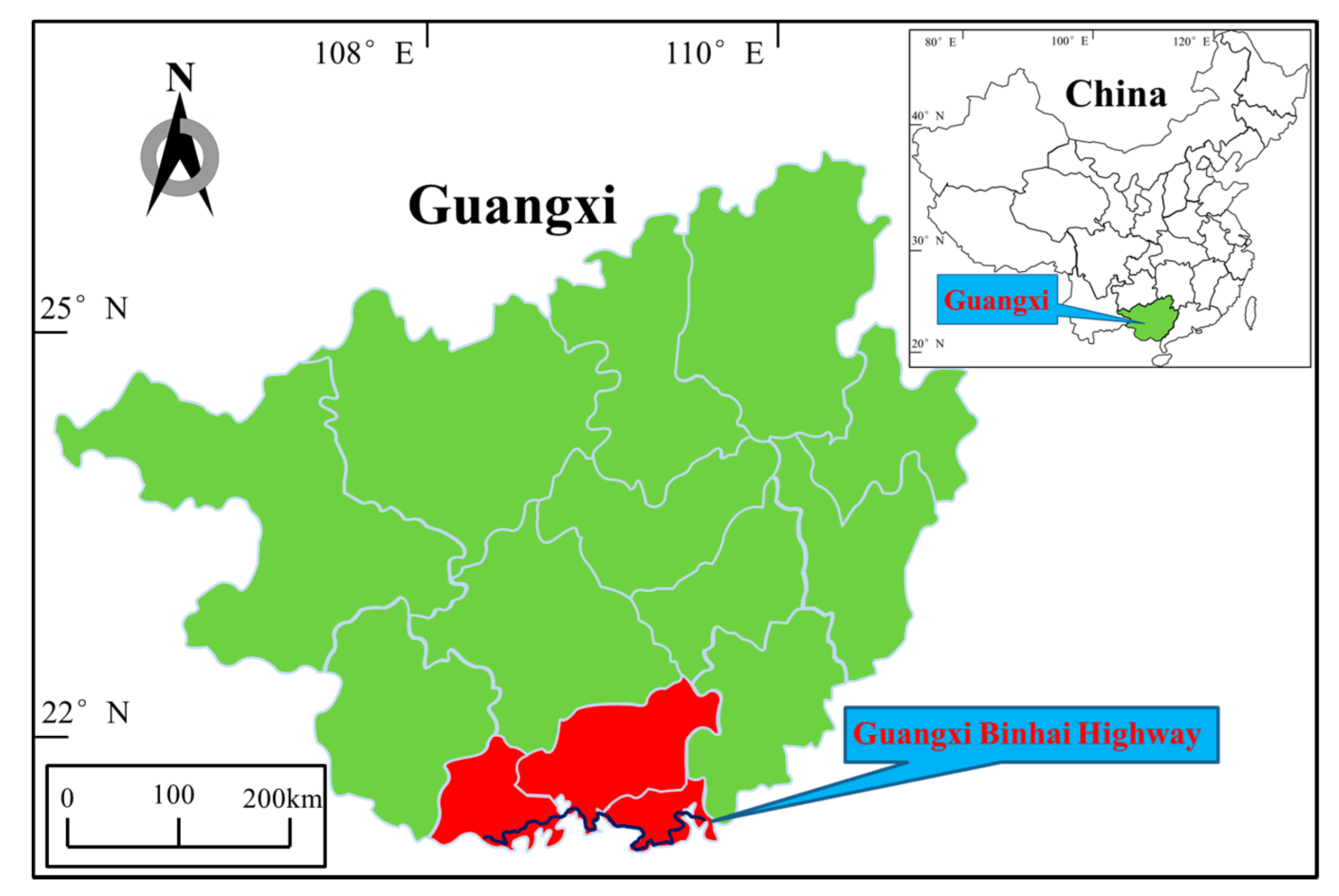
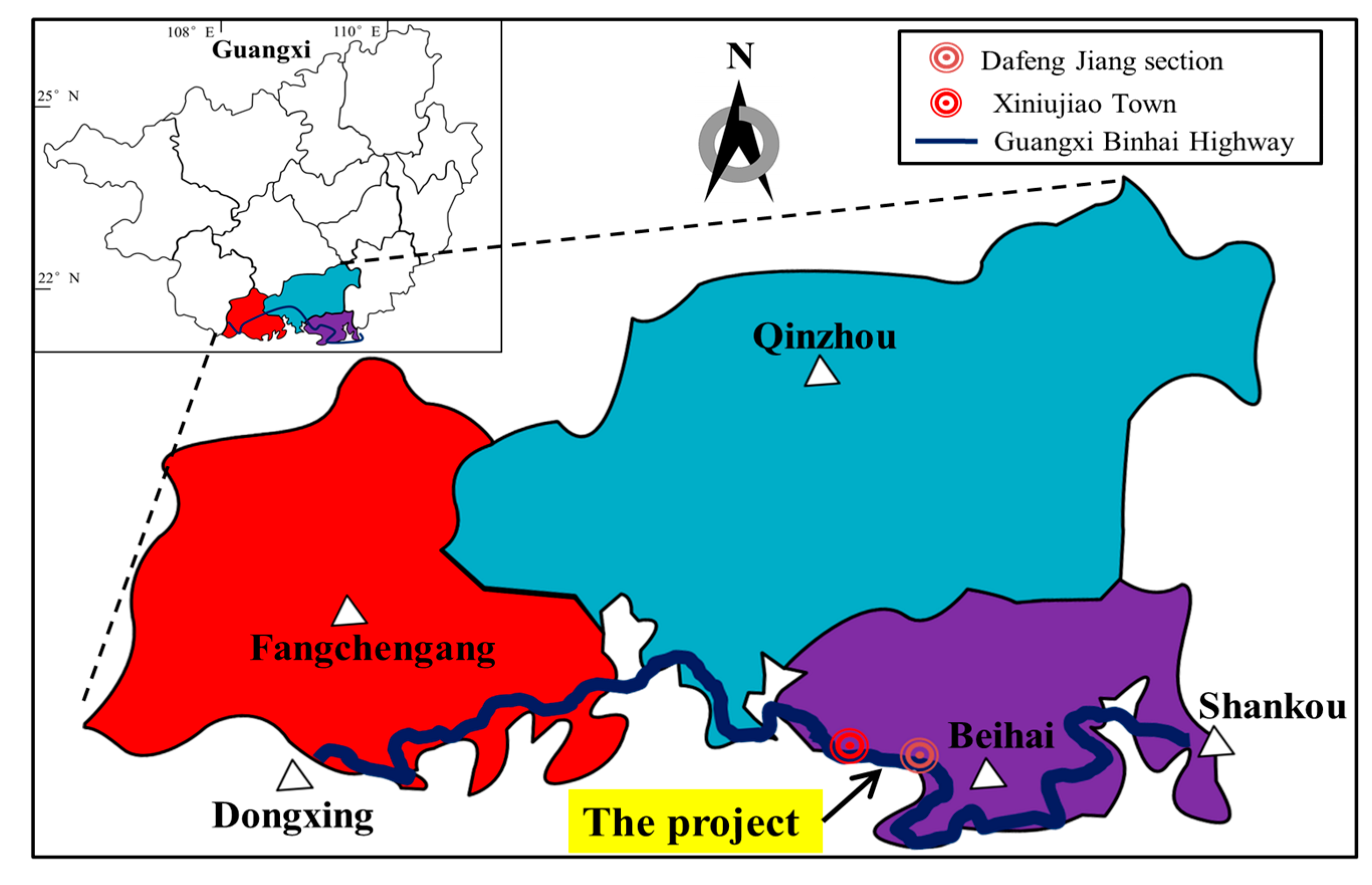
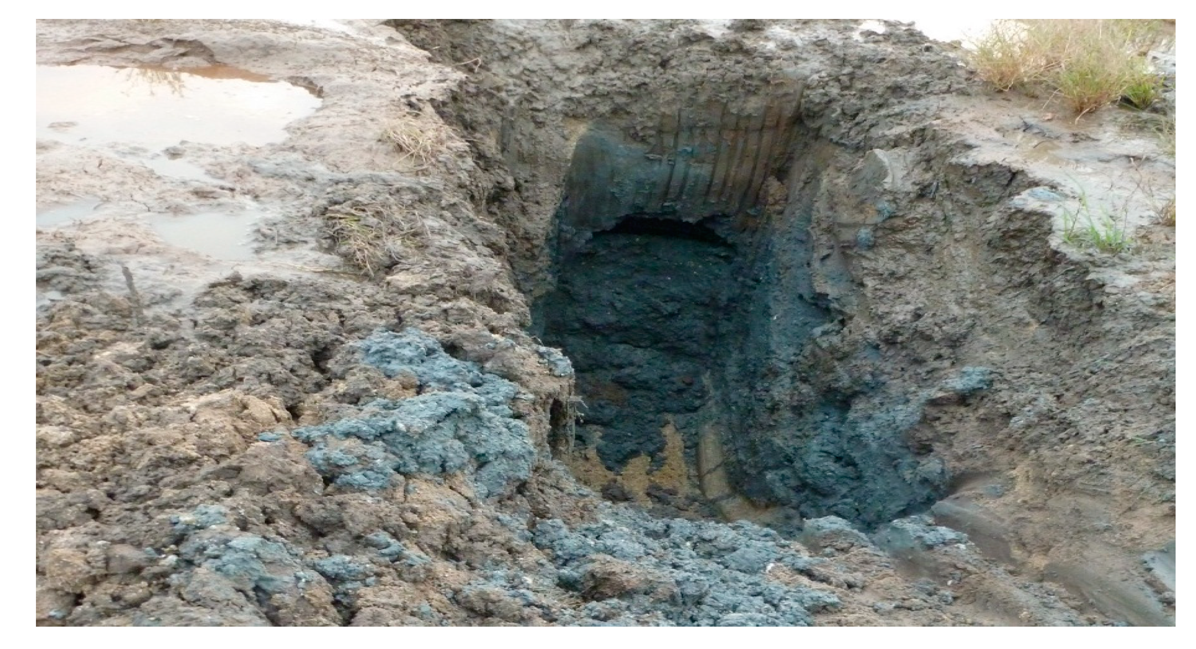
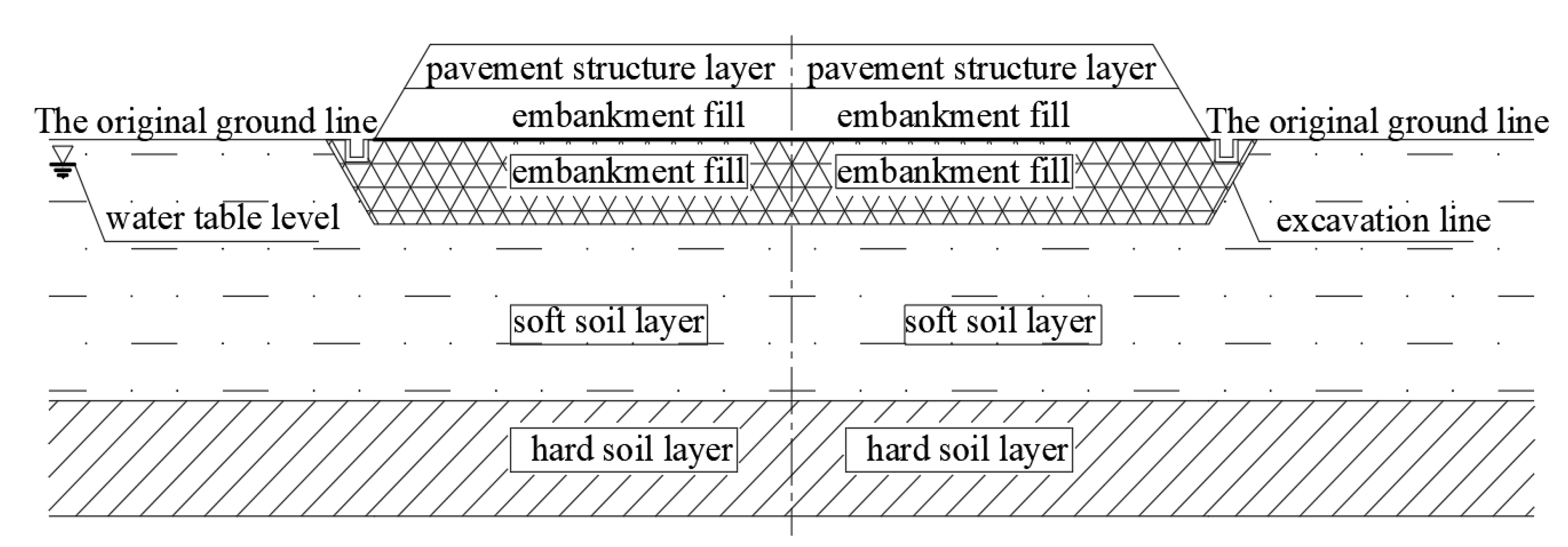
4.1. Project Overview
4.2. Settlement and Consolidation Analysis
5. Conclusions
- (1)
- Considering the complex drainage boundary conditions, combining the continuous drainage boundary conditions theory, the improved double-layer soil consolidation theory is derived by using the Laplace transform and Stehfest algorithm with high computational efficiency.
- (2)
- Based on the improved double-layer soil consolidation theory, the perfectly permeable boundary case and the semi-permeable boundary case are used to verify this theory. The calculation results are basically consistent with Xie’s solution, and it is concluded that the improved double-layer soil consolidation model proposed in the present paper had higher accuracy.
- (3)
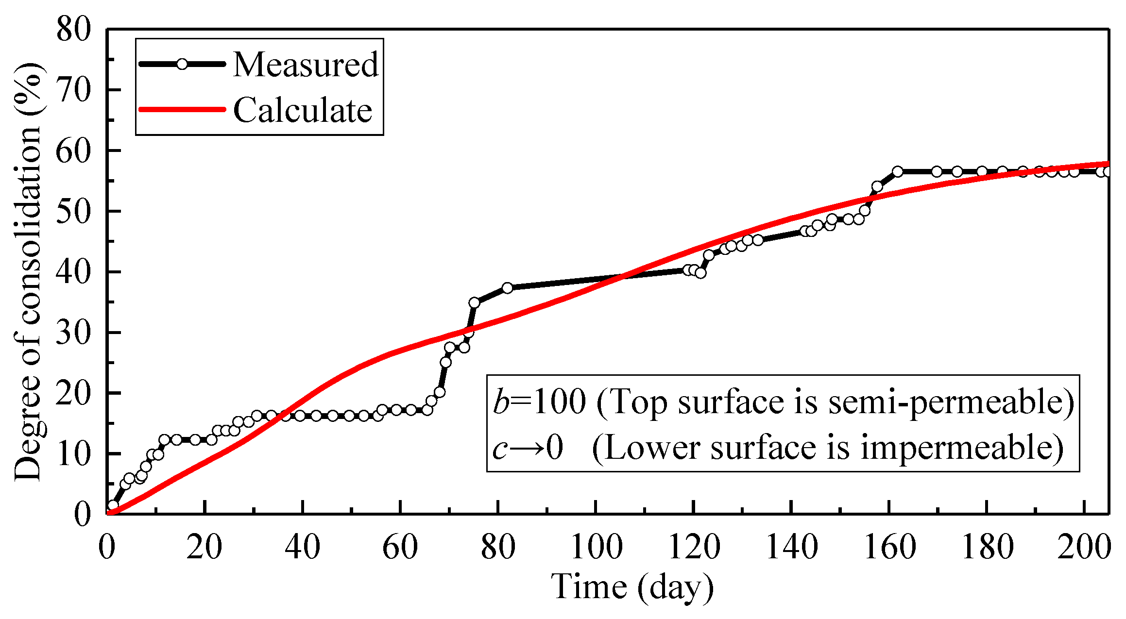
- The improved double-layer soil consolidation theory is used in an actual engineering case of marine soft soil in Guangxi. Compared with the measured data, the error of calculated data is 0.7–2.3%. The calculated results are basically consistent with the measured results, indicating that this theory is suitable for the analysis of consolidation and settlement of marine soft soil foundation with complex drainage conditions.
- (4)
- It is difficult to quantitatively control the drainage parameters of the improved double-layer soil consolidation theory, which requires a large number of practical cases to determine the parameters. Only the double-layer foundation has been studied here, and soft foundation with more layers needs further study.
Author Contributions
Funding
Acknowledgments
Conflicts of Interest
Nomenclature
| Symbol | Description | Units |
| The undetermined constant in Equation (17) | [-] | |
| The undetermined constant in Equation (18) | [-] | |
| Related to the drainage property of topsoil | [-] | |
| c | Related to the drainage property of subsoil | [-] |
| Consolidation coefficients of the first/second layer | [m2/s] | |
| Compression modulus of the first/second layer | [Pa] | |
| Laplace function of , | - | |
| Time domain function of | - | |
| An approximation of the inverse Laplace transform of | - | |
| Thickness of the first/second layer | [m] | |
| i | The process variable of accumulation equation | - |
| k | The process variable of accumulation equation | - |
| Permeability coefficients of the first/second layer | [m/s] | |
| Positive even number | [-] | |
| Arbitrary loading function | [Pa] | |
| Load increments at the first/second levels | [Pa] | |
| Total consolidation settlement at time of foundation | [m] | |
| Final total consolidation settlement of foundation | [m] | |
| Intermediate variable, no real meaning | [/m] | |
| Complex variable involved in the Laplace transform | [/s] | |
| Time | [s] | |
| Loading time of first class load | [s] | |
| Starting time of the second stage load | [s] | |
| Completion time of the second stage load | [s] | |
| Excess pore water pressure | [Pa] | |
| Average degree of consolidation of foundation | [-] | |
| Excess pore water pressure of the first/second layer | [Pa] | |
| Derivative of with respect to | - | |
| Dependent on N only | [-] | |
| Foundation depth, from the ground up | [m] | |
| Water unit weight, take 104 N/m3 | [N/m3] | |
| Effective stress of the first/second layer | [Pa] | |
| Effective stress at any point in the foundation at any time | [Pa] |
Appendix A
References
- Boak, E.H.; Turner, I.L. Shoreline Definition and Detection: A Review. J. Coast. Res. 2005, 21, 688–703. [Google Scholar] [CrossRef]
- Penner, E. A Study of Sensitivity in Leda Clay. Can. J. Earth Sci. 1965, 2, 425–441. [Google Scholar] [CrossRef]
- Gillott, J.E. Clay, Engineering Geology; Springer: New York, NY, USA, 1984. [Google Scholar]
- Sangrey, D.A. Naturally Cemented Sensitive Soils. Géotechnique 1972, 22, 139–152. [Google Scholar] [CrossRef]
- Gasparre, A.; Nishimura, S.; Jardine, R.J.; Coop, M.R.; Minh, N.A. The Stiffness of Natural London Clay. Géotechnique 2007, 57, 33–47. [Google Scholar] [CrossRef]
- Dìaz-Rodrìguez, J.A.; Leroueil, S.; Alemàn, J.D. Yielding of Mexico City Clay and Other Natural Clays. J. Geotech. Eng. 1992, 118, 981–995. [Google Scholar] [CrossRef]
- Aoki, S.; Oinuma, K. The Distribution of Clay Minerals in Recent Sediments of the Okhotsk Sea. Deep Sea Res. Oceanogr. Abstr. 1974, 21, 299–310. [Google Scholar] [CrossRef]
- Kim, Y.T.; Nguyen, B.P.; Yun, D.H. Effect of Artesian Pressure on Consolidation Behavior of Drainage-Installed Marine Clay Deposit. ASCE’s J. Mater. Civ. Eng. 2018, 30, 04018156. [Google Scholar] [CrossRef]
- Yin, L.H.; Wang, X.M.; Zhang, L.J. Probabilistical Distribution Statistical Analysis of Tianjin Soft Soil Indices. Rock Soil Mech. 2010, 31, 462–469. (In Chinese) [Google Scholar]
- Li, X.G.; Xu, R.Q.; Wang, X.C.; Rong, X.N. Assessment of Engineering Properties for Marine and Lacustrine Soft Soil in Hangzhou. J. Zhejiang Univ. (Eng. Sci.) 2013. (In Chinese) [Google Scholar]
- Liang, S.J.; Zhu, H.D. Statistical Analysis on Soil Indices of Lagoon Facies Soft Soil Layer in Hangzhou. Subgrade Eng. 2012. (In Chinese) [Google Scholar]
- Zheng, Y.Y.; Zhu, J.F.; Liu, G.B.; Jia, B. Probability and Correlation between Physical and Mechanical Parameters of Soft Clays in Ningbo Rail Transit Engineering. China Sciencepaper 2013, 8, 367–373. (In Chinese) [Google Scholar]
- Chen, X.P.; Huang, G.Y.; Liang, Z.S. Study on Soft Soil Properties of the Pearl River Delta. Chin. J. Rock Mech. Eng. 2003, 22, 137–141. (In Chinese) [Google Scholar]
- Lei, D.; Jiang, Y.J.; Chen, D.C.; Zhang, X.Y. Mechanical Properties and Correlation Analysis of Soft Soil in Guangzhou. Railway Eng. 2011, 10, 75–78. (In Chinese) [Google Scholar]
- Zhu, W.D. Engineering Properties and Comparison Analysis of Wen Zhou Soft Clay and Tai Zhou Soft Clays. Zhejiang Univ. 2003. (In Chinese) [Google Scholar]
- Luo, Y.D.; Yang, G.H.; Zhang, Y.C.; Liu, P. Engineering Characteristics and Its Statistical Analysis of Soft Marine Clay on Shenzhen West Coast. J. Civ. Eng. Manag. 2012, 29, 79–86. (In Chinese) [Google Scholar]
- Terzaghi, K. Theoretical Soil Mechanics; John Wiley and Sons: New York, NY, USA, 1943. [Google Scholar]
- Xie, K.H.; Xie, X.Y.; Gao, X. Theory of One Dimensional Consolidation of Two Layered with Partially Drained Boundaries. Comput. Geotech. 1999, 24, 265–278. [Google Scholar] [CrossRef]
- Zhou, W.H.; Zhao, L.S. One-Dimensional Consolidation of Unsaturated Soil Subjected to Time-Dependent Loading with Various Initial and Boundary Conditions. Int. J. Geomech. 2014, 14, 291–301. [Google Scholar] [CrossRef]
- Gray, H. Simultaneous Consolidation of Contiguous Layers of Unlike Compressible Soils. Am. Soc. Civ. Eng. 1945, 110, 1327–1356. [Google Scholar]
- Schiffman, R.L.; Stein, J.R. One-Dimensional Consolidation of Layered Systems. JSM FD ASCE 1970, 96, 1499–1504. [Google Scholar]
- Huang, W.X. Application of Consolidation Theory to Earth Dams Built by Sluicing-Siltation Method. J. Hydraul. Eng. 1982, 9, 13–23. (In Chinese) [Google Scholar]
- Xie, K.H. One Dimensional Consolidation Analysis of Layered Soils with Impeded Boundaries. J. Zhejiang Univ. (Eng. Sci.) 1996. (In Chinese) [Google Scholar]
- Hu, L.H.; Xie, K.H. On One Dimensional Consolidation Behavior of Layered Soil with Partial Drainage Boundaries. Bull. Sci. Technol. 2005. (In Chinese) [Google Scholar]
- Feng, Y.; Xu, C.J.; Cai, Y.Q. One-Dimensional Consolidation Analysis of Saturated Gibson Soils with Semi-Pervious Boundaries. J. Zhejiang Univ. (Eng. Sci.) 2003, 37, 646–651. (In Chinese) [Google Scholar]
- Lin, Z.Y.; Pan, W.X.; Xu, C.J. One-Dimensional Consolidation Analysis of Saturated Layered Gibson Soils with Semi-Pervious Boundaries. J. Zhejiang Univ. (Eng. Sci.) 2003, 37, 570–575. (In Chinese) [Google Scholar]
- Wang, K.H.; Xie, K.H.; Zeng, G.X. A Study on 1D Consolidation of Soils Exhibiting Rheological Characteristics with Impeded Boundaries. Chin. J. Geotech. Eng. 1998. (In Chinese) [Google Scholar]
- Wang, L.; Li, L.Z.; Xu, Y.F.; Xia, X.H.; Sun, D.A. Analysis of One-Dimensional Consolidation of Fractional Viscoelastic Saturated Soils with Semi-Permeable Boundary. Rock Soil Mech. 2018, 39, 234–240. (In Chinese) [Google Scholar]
- Cai, Y.Q.; Liang, X.; Zheng, Z.F.; Pan, X.D. One-Dimensional Consolidation of Viscoelastic Soils Layer with Semi-Permeable Boundaries under Cyclic Loadings. China Civ. Eng. J. 2003, 36, 86–90. (In Chinese) [Google Scholar]
- Li, X.B.; Xie, K.H.; Wang, K.H.; Zhuang, Y.C. Analytical Solution of 1-D Visco-Elastic Consolidation of Soils with Impeded Boundaries under Cyclic Loadings. Eng. Mech. 2004, 21, 103–108. (In Chinese) [Google Scholar]
- Wang, W.G.; Xia, S.W. On Analytical Solutions to Viscoelastic One-Dimensional Consolidation of Impeded Boundaries under Cyclic Loading. Shanxi Archit. 2011, 37, 67–69. (In Chinese) [Google Scholar]
- Zheng, Z.F.; Cai, Y.Q.; Xu, C.J.; Zhan, H. One-Dimensional Consolidation of Layered and Visco-Elastic Ground under Arbitrary Loading with Impeded Boundaries. J. Zhejiang Univ. (Eng. Sci.) 2005, 39, 1234–1237. (In Chinese) [Google Scholar]
- Cheng, Z.H.; Chen, Y.M.; Ling, D.S.; Lv, F.R. Analytical Solutions for Consolidation Problems with Impeded Boundaries. Acta Mech. Solida Sin. 2004, 25, 93–97. (In Chinese) [Google Scholar]
- Liu, J.C.; Lei, G.G.; Wang, Y.X. One-Dimensional Consolidation of Soft Ground Considering non-Darcy Flows. Chin. J. Geotech. Eng. 2011, 33, 1117–1122. (In Chinese) [Google Scholar]
- Mei, G.X.; Xia, J.; Mei, L. Terzaghi’s One-Dimensional Consolidation Equation and its Solution based on Asymmetric Continuous Drainage Boundary. Chin. J. Geotech. Eng. 2011, 1, 28–31. (In Chinese) [Google Scholar]
- Zong, M.F.; Wu, W.B.; Mei, G.X.; Liang, R.Z. An Analytical Solution for One-Dimensional Nonlinear Consolidation of Soils with Continuous Drainage Boundary. Chin. J. Rock Mech. Eng. 2018, 37, 2829–2838. (In Chinese) [Google Scholar]
- Zheng, Y.; Mei, G.X.; Mei, L. Generalized Continuous Drainage Boundary Applied in One-Dimensional Consolidation Theory. J. Nanjing Univ. Technol. (Nat. Sci. Ed.) 2010, 32, 54–58. (In Chinese) [Google Scholar]
- Cai, F.; He, L.J.; Zhou, X.P.; Mei, G.X. Finite Element Analysis of One-Dimensional Consolidation Problem with Continuous Drainage Boundaries in Layered Ground. J. Cent. South Univ. (Sci. Technol.) 2013, 44, 315–323. (In Chinese) [Google Scholar]
- Wang, L.; Sun, D.A.; Qin, A.F. Semi-Analytical Solution to One-Dimensional Consolidation for Unsaturated Soils with Exponentially Time-Growing Drainage Boundary Conditions. Int. J. Geomech. 2018, 18, 04017144. [Google Scholar] [CrossRef]
- Feng, J.X.; Ni, P.P.; Mei, G.X. One-Dimensional Self-Weight Consolidation with Continuous Drainage Boundary Conditions: Solution and Application to Clay-Drain Reclamation. Int. J. Numer. Anal. Methods Geomech. 2019, 1–19. [Google Scholar] [CrossRef]
- Sun, M.; Zong, M.F.; Ma, S.J.; Wu, W.B.; Liang, R.Z. Analytical Solution for One-Dimensional Consolidation of Soil with Exponentially Time-Growing Drainage Boundary under a Ramp Load. Math. Probl. Eng. 2018. [Google Scholar] [CrossRef]
- Zhang, Y.; Wu, W.B.; Mei, G.X.; Duan, L.C. Three-Dimensional Consolidation Theory of Vertical Drain Based on Continuous Drainage Boundary. J. Civ. Eng. Manag. 2019, 25, 145–155. [Google Scholar] [CrossRef]
- Van Everdingen, A.F.; Hurst, W. The Application of the Laplace Transformation to Flow Problems in Reservoirs. J. Pet. Technol. 1949, 186, 305–324. [Google Scholar] [CrossRef]
- Dubner, H.; Abate, J. Numerical Inversion of Laplace Transforms by Relating Them to the Finite Fourier Cosine Transform. J. ACM 1968, 15, 115–123. [Google Scholar] [CrossRef]
- Durbin, F. Numerical Inversion of Laplace Transforms: An Efficient Improvement to Dubner and Abate’s Method. Comput. J. 1974, 17, 371–376. [Google Scholar] [CrossRef]
- Stehfest, H. Algorithm 368: Numerical Inversion of Laplace Transforms [D5]. Commun. ACM 1970, 13, 47–49. [Google Scholar] [CrossRef]
- Stehfest, H. Remark on Algorithm 368: Numerical Inversion of Laplace Transforms. Commun. ACM 1970, 13, 624. [Google Scholar] [CrossRef]
- Crump, K.S. Numerical Inversion of Laplace Transforms Using a Fourier Series Approximation. J. ACM 1976, 23, 89–96. [Google Scholar] [CrossRef]
- Duffy, D.G. On the Numerical Inversion of Laplace Transforms: Comparison of Three New Methods on Characteristic Problems from Applications. ACM Trans. Math. Softw. 1993, 19, 333–359. [Google Scholar] [CrossRef]
- Wang, X.H.; Miao, L.C.; Gao, J.K.; Zhao, M. Solution of One-Dimensional Consolidation for Double-Layered Ground by Laplace Transform. Rock Soil Mech. 2005, 26, 833–836. (In Chinese) [Google Scholar]
- Xie, K.H. One Dimensional Consolidation Theory of Double-Layered Ground. Chin. J. Geotech. Eng. 1994, 5, 24–35. (In Chinese) [Google Scholar]


| Value | 0 | (0, +∞) | +∞ | |
|---|---|---|---|---|
| Parameter | ||||
| b | impermeable | semi-permeable | perfectly permeable | |
| c | impermeable | semi-permeable | perfectly permeable | |
| Layer | Layer Thickness h (m) | Permeability Coefficient k (10−8m/s) | Compression Modulus Es (MPa) |
|---|---|---|---|
| Topsoil | 1 | 1.014 | 8 |
| Subsoil | 9 | 2.028 | 4 |
| Layer | Layer Thickness h (m) | Permeability Coefficient k (10−9 m/s) | Compression Modulus Es (MPa) |
|---|---|---|---|
| Topsoil | 3 | 1 | 8 |
| Subsoil | 3 | 5 | 1.6 |
| Layer | Layer Thickness (m) | Bulk Unit Weight (kN/m3) | Water Content (%) | Liquid Limit (%) | Cohesion (kPa) | Friction Angle (°) | Compression Modulus (MPa) | Permeability Coefficient (10−8m/s) | SPT |
|---|---|---|---|---|---|---|---|---|---|
| Crust layer | 3 | 18.8 | 20.6 | 35.7 | 25.2 | 18.7 | 15 | 3.8 | 7 |
| Soft soil layer | 7 | 16.7 | 45.2 | 36.7 | 4.5 | 8.6 | 7.0 | 3.0 | 6 |
| Filling in granite | - | 26 | - | - | 150 | 45 | 1200 | 5 × 10⁴ | >50 |
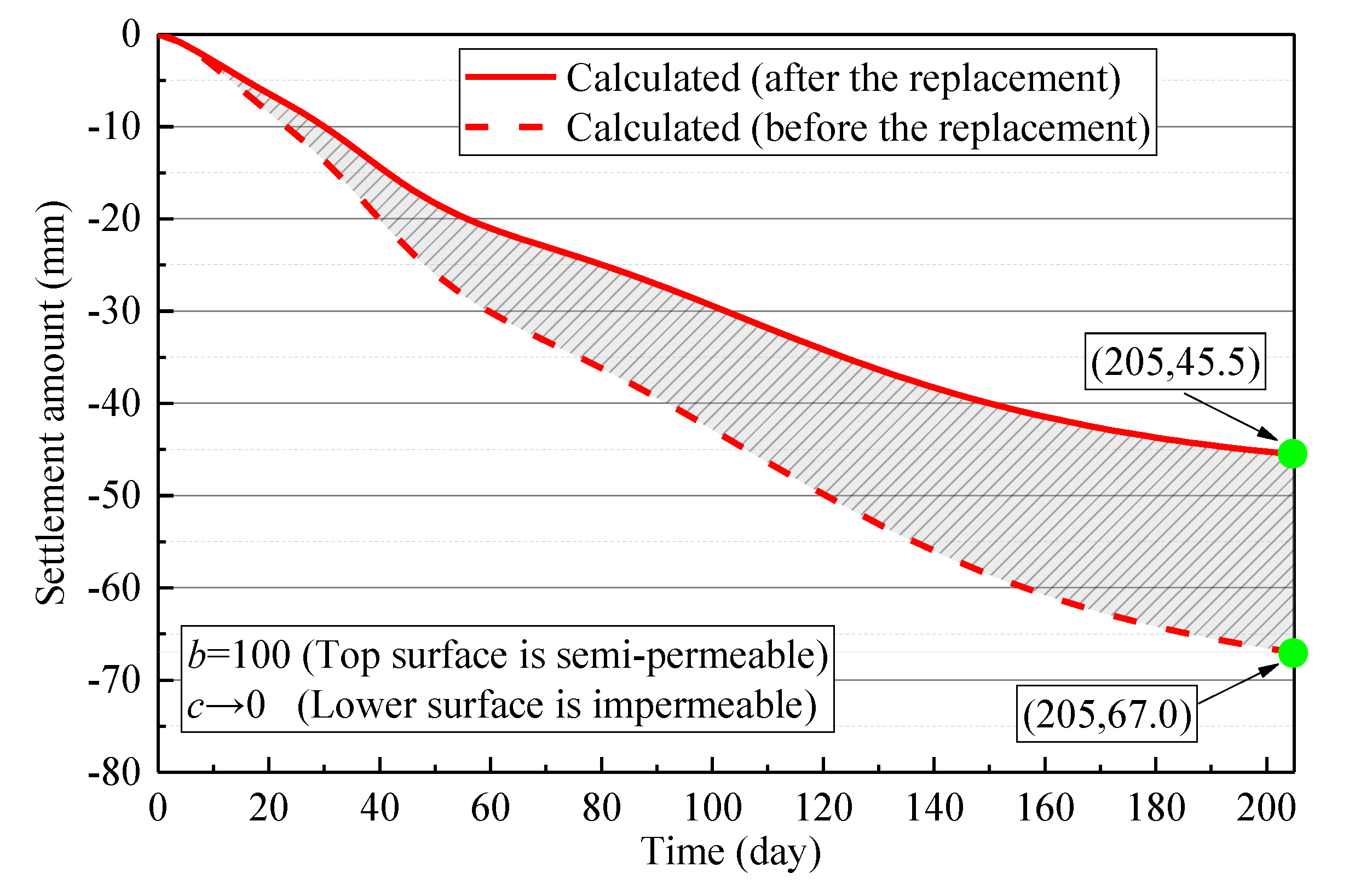
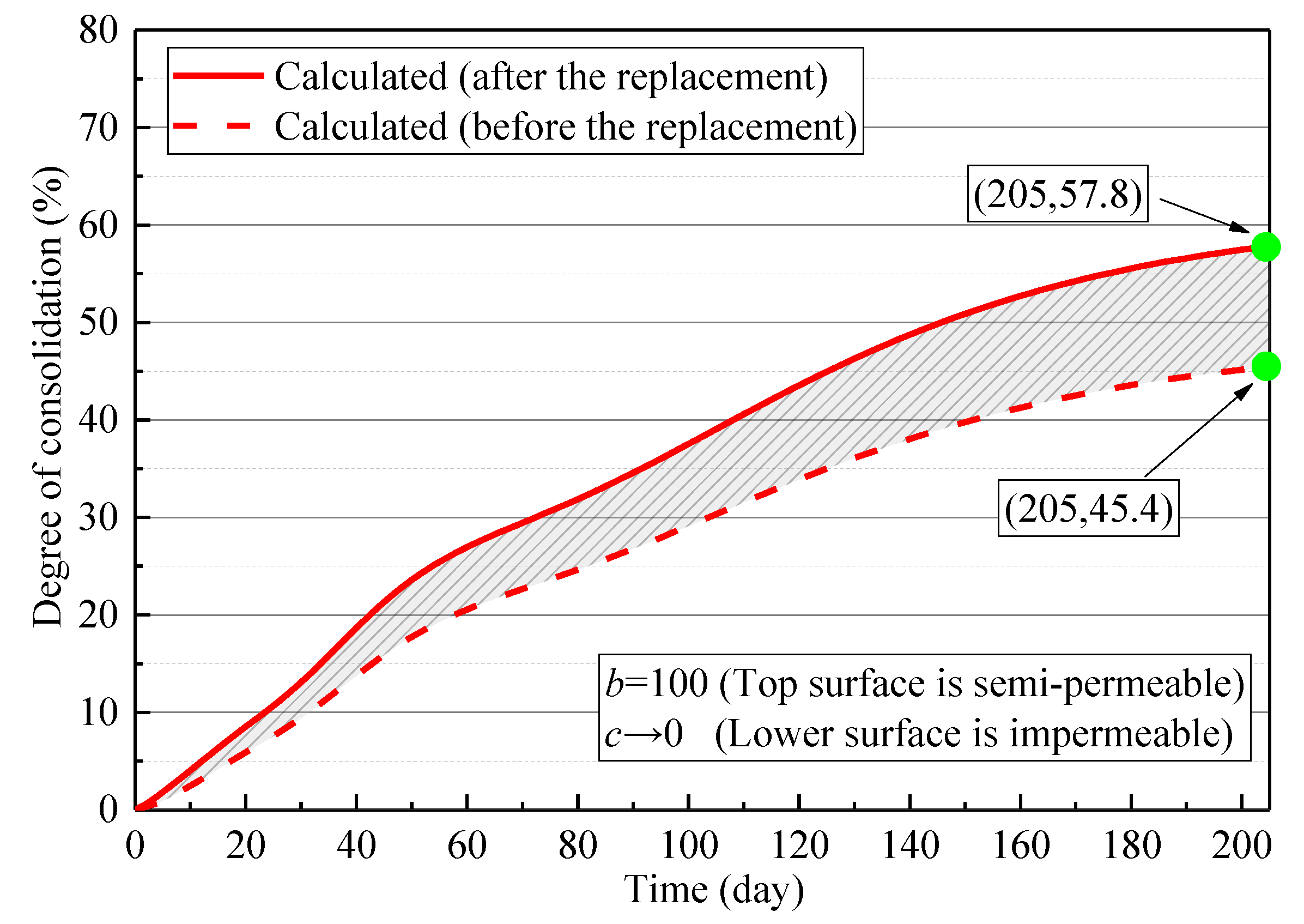
| Data Source | Final Settlement (mm) | Settlement (mm) After 205 Days | Consolidation Degree (%) After 205 Days |
|---|---|---|---|
| Measured data | 80.0 | 45.2 | 56.5 |
| Calculated data (after the replacement) | 78.7 | 45.5 | 57.8 |
| Calculated data (before the replacement) | 147.6 | 67.0 | 45.4 |
© 2019 by the authors. Licensee MDPI, Basel, Switzerland. This article is an open access article distributed under the terms and conditions of the Creative Commons Attribution (CC BY) license (http://creativecommons.org/licenses/by/4.0/).
Share and Cite
Chen, D.; Luo, J.; Liu, X.; Mi, D.; Xu, L. Improved Double-Layer Soil Consolidation Theory and Its Application in Marine Soft Soil Engineering. J. Mar. Sci. Eng. 2019, 7, 156. https://doi.org/10.3390/jmse7050156
Chen D, Luo J, Liu X, Mi D, Xu L. Improved Double-Layer Soil Consolidation Theory and Its Application in Marine Soft Soil Engineering. Journal of Marine Science and Engineering. 2019; 7(5):156. https://doi.org/10.3390/jmse7050156
Chicago/Turabian StyleChen, Deqiang, Junhui Luo, Xianlin Liu, Decai Mi, and Longwang Xu. 2019. "Improved Double-Layer Soil Consolidation Theory and Its Application in Marine Soft Soil Engineering" Journal of Marine Science and Engineering 7, no. 5: 156. https://doi.org/10.3390/jmse7050156
APA StyleChen, D., Luo, J., Liu, X., Mi, D., & Xu, L. (2019). Improved Double-Layer Soil Consolidation Theory and Its Application in Marine Soft Soil Engineering. Journal of Marine Science and Engineering, 7(5), 156. https://doi.org/10.3390/jmse7050156