Variations in Winter Ocean Wave Climate in the Japan Sea under the Global Warming Condition

Abstract

Future variations in the ocean wave climate caused by global warming could affect various coastal issues. Using a third-generation wave model, this study produced projections of the ocean wave climate for winter around Japan, focusing on the Japan Sea side. Wave simulation forcing (sea surface wind) was generated through five different global warming experiments. More than half the future wave projections showed an increasing tendency of the climatological mean significant wave height during winter. However, the maximum significant wave height did not show any clear tendency in future variation. The top 1% of significant wave heights and mean wave periods showed apparent increases in frequencies of higher/longer waves in three out of the five future projections. Frequency distributions of significant wave height, mean wave period, mean wavelength and wave direction showed various future variations (reduction of small ocean waves, increasing frequency of waves from the west). There are large uncertainties in future variations of wave climate in the Japan Sea, but the high probability of variations in daily wave climate is recognized, based on the future wave projections. Variations in daily wave climate are important because they could affect the topography and environment of the coast through long-term repetitive actions.

1. Introduction

Variations in the atmospheric conditions because of climate change could have impacts on the ocean wave climate. Variations in ocean wave climate, including mean and extreme wave conditions, could have considerable impact on various applications, e.g., coastal planning (flood disaster prevention, coastal environment), design of coastal and offshore structures, ship design, harbor activities, and the evaluation of wave energy resources. Projections of future wave climate are indispensable for the assessment of the impact of variations in wave climate and for the development of appropriate adaptation strategies. However, Global Climate Models (GCMs) for climate research do not simulate ocean waves, and some postprocessing or analysis method is necessary to investigate the effects of climate change on ocean waves. Projections with high spatial resolution are desirable especially for detail assessment of the impact on wave climate for specific coastal areas.

There are two approaches to generate projections of wave climate. One is dynamical downscaling based on numerical models, and another one is statistical downscaling technique. In both approaches, atmospheric conditions (near-surface wind and/or sea level pressure) projected by GCMs are used to generate ocean wave conditions.

Seasonal mean and extreme global ocean wave heights were projected with sea level pressure projected by multiple GCMs and emission scenarios as forcing [1]. A statistical downscaling method was applied using a regression model, and the projected ocean wave height was estimated on a 96–48 Gaussian grid in [1]. Future variations of global ocean wave climate were examined with ocean wave heights projections by another statistical method by the authors of [2]. The sea level pressure from 20 GCMs in the Coupled Model Intercomparison Project Phase 5 (CMIP5 [3]) were used to generate the ocean wave projections with spatial resolution of 2.0° × 2.0° [2]. A statistical method for different weather types was developed and future variations of the wave climate in Europe were investigated in [4]. The three-day average sea level pressure and sea level pressure gradient were used as predictors and the mean wave heights were projected in their method. Using dynamical methods, global wave climate was projected by a wave model with the resolutions of 1.25° and the variations in the mean and the extreme wave climate were examined in [5]. Different tendencies of future variations of wave climate were found in different regions (including the seas around Japan) [5]. The spatial resolutions in above studies were too coarse to examine the details in relation to the Japan Sea.

The variations in ocean waves in the Bay of Biscay were examined by wave simulations with the spatial resolution of 0.1° in [6]. Both downscaling by the wave model and error correction were applied in [6]. Decreasing winter wave height was found according to a decrease of wind speed in the central North Atlantic Ocean and the Bay of Biscay. Future projections of the wave climate were generated by a third-generation wave model (WAM) with resolution of 0.05° × 0.075 ° with two initial conditions and two emission scenarios [7]. Variations of the wave direction were larger than variations of the wave height in the North Sea. Ten future projections showed an increasing mean and extreme wave heights in eastern parts of the North Sea but decrease in western parts [8]. A spectral wave model was used with forcing data from GCM projections with 1.0° × 1.0° spatial resolution in [9]. Increases of the wave generation and the mean significant wave height in the Southern Ocean and decrease of the wave generation with comparable wave height in the North Atlantic Ocean were reported in [9]. Variations in the global wave climate were examined using simulation results from a wave model with forcing from a GCM projection [10]. The changes of wave climate in different regions and seasons were discussed in [10]. Global swell and wind–sea characteristics at the end of the 21st century were investigated by using the results of a coupled atmosphere-ocean wave simulation system with the resolution of 0.5° × 0.5° [11]. Wave climate in the Pacific Ocean was examined with wave simulations based on the multiple emission scenarios of two different GCMs with 0.25° × 0.25° resolution [12]. Mean and extreme wave heights decreased along the west coast of North America in [12]. For the western North Pacific Ocean, 0.5° × 0.5° resolution wave simulations were generated and the effects of sea surface temperature conditions were investigated to understand the mechanism behind changes in wave climate [13].

Finer resolution wave climates by statistical and dynamical downscaling methods were compared by the authors of [14]. The results from the dynamical method were slightly closer to the observations, and the difference between the dynamical and the statistical methods was larger under more severe global warming conditions [14]. In addition, statistical methods showed disadvantages in the estimation of extreme wave events [14]. Another comparison of statistical and dynamical downscaling method showed that statistical projection using climate indices (sea level pressure and/or pressure gradient) did not reproduce long-term trend in the North Atlantic wave climate [15]. Another disadvantage of the statistical downscaling methods is that it does not consider swell effects [16]. Thus, dynamical methods could be more appropriate for evaluation of global warming impact in more energetic conditions.

The direct use of GCM output as wave model forcing could cause overestimation of swell in broad regions of the Southern Pacific Ocean [9]. Large negative biases were also recognized in wave simulation with direct use of CMIP5 GCM output as forcing [17]. To prevent such defects of using GCMs output directly in downscaling, a pseudo global warming (PGW) method [18] was applied in this study. The PGW conditions are generated by adding future anomalies from the GCM output to reanalysis data. Then, simulations forced by PGW conditions are made and compared with simulations forced by reanalysis data (more accurate forcing than the direct use of GCMs).

Strong seasonal northwesterly winds prevail during winter over the Japan Sea, which can make sea conditions difficult. Sometimes, a large swell can be generated by the passage of an intense low-pressure system. For example, in 2008, a very large swell exceeding 9.9 m affected Toyama Bay (northern Honshu, Japan). In this study, a dynamical method was applied for the Japan Sea. The wind output of a numerical model was used as the forcing data in a wave simulation. For the present climate, winds simulated with reanalysis data were used. For the future climate, the results of PGW simulations implemented using multiple GCM products were used as the forcing for the wave simulations.

The remainder of this paper is organized as follows. In Section 2, the data and wave model used in this study are described. In Section 3, the results and a discussion of wave simulations are presented. Finally, in Section 4, a summary of the study is provided.

2. Methods

2.1. Forcing Data forWave Simulations

As forcing data for the wave model, this study used the results of dynamic downscaling by a numerical weather prediction model. Future variations of precipitation in the Kanto Region of Japan were investigated in [19]. Future precipitation characteristics were obtained by dynamic downscaling with PGW conditions, which were compared with the downscaling results of present climate condition forced by reanalysis data. The Weather Research and Forecasting model (WRF, [20]) version 3.4 was used for downscaling in [19]. For downscaling of present climate, Japanese 25-year reanalysis (JRA-25, [21]) were used as initial and boundary conditions. As forcing of downscaling future climate by WRF, the PGW conditions were obtained from five different global warming experiments as part of CMIP5 (listed in

Table 1. List of Coupled Model Intercomparison Project Phase 5 (CMIP5) model output used in this study.

No.	IPCC ID	Institute and Country	Resolution
1	CNRM-CM5	Meteo-France, Centre Nationale de Resherches Meteorologique (France)	T127, L31
2	GFDL-CM3	Geophysical Fluid Dynamics Laboratory (USA)	2.0° × 2.0°, L48
3	GISS-E2-R	NASA/Goddard Institute for Space Studies (USA)	2.0° × 2.5°deg, L40
4	MIROC5	Center for Climate System Research (University of Tokyo), National Institute for Environmental Studies, and Frontier Research Center for Global Change (Japan)	T85, L40
5	MRI-CGCM3	Meteorological Research Institute, Japan Meteorological Agency (Japan)	T159, L48

). The climatological spatial patterns of atmospheric temperature and specific humidity around Japan are well-reproduced with the correlation coefficient higher than 0.8 in these five GCMs [19]. In the preparation of the PGW conditions, high temporal resolution (6 hourly) anomalies were produced as the differences between the 6-hourly future atmospheric conditions and the climatological monthly mean conditions of historical runs in each of the GCMs. Then, the PGW conditions were generated by adding the anomalies to the monthly mean climatology based on JRA-25. The historical climatological monthly mean conditions were taken as the 1996–2005 (or 2001–2010 for some GCMs output) averages, and the future conditions were taken as the 6-hourly products from 2060 to 2070 under the RCP4.5 emission scenario [3]. All the PGW conditions were based on the same climatological conditions (or JRA-25). Thus, the PGW method allows comparison of the results of one historical downscaling and multiple future conditions. Dynamic downscaling for the historical period was implemented for the period 2000–2010. The period of the historical downscaling (2000–2010) and the period to make the historical climatological monthly mean conditions (1996–2005 or 2001–2010) are different. But the difference between these periods are not significant to investigate climatological features. In the downscaling simulation by WRF, a two-domains nesting system was applied. The horizontal spatial resolutions of the parent and child domains were 30 km and 6 km, respectively [19].

In this study, the wave model was forced by zonal and meridional wind components at 10 m above the ground surface, which were obtained as dynamic downscaling results in [19]. Eleven years’ output for the present (2000–2010) and future (2060–2070) periods were used for the wave simulation.

In [19], PGW conditions were produced with projections from the five GCMs listed in Table 1. In this study, the wave simulations forced by future projections were named PGW-1, 2, …, 5 with the number of the GCM shown in Table 1. The historical wave simulation (or the results of the present climate) was called CTL.

2.2. Wave Simulation (WaveWatch III)

WaveWatchIII (hereafter, WW3) is a third-generation spectral wave model that was developed by NOAA/NCEP [22]. Wave climate around Japan was projected by WW3 with the forcing of wind speed from downscaling results mentioned in the previous section. A nesting method was applied to obtain high resolution wave climate along the coast on the Japan Sea. The parent domain, with a 0.1° resolution, covered the sea area around all parts of Japan. The inner domain had 0.033° horizontal resolution and covered the sea area from the central to northern parts of the coast on the Japan Sea side (Figure 1). In the simulations, 24 wave directions were set with 15° intervals. Twenty-four wave frequencies were set from 0.04118 to 0.44617 Hz using an incremental factor of 1.1. The n-th frequency $f\left(n\right)$ is expressed by

$$f\left(n+1\right)=1.1f\left(n\right).$$

(1)

For flux computation, following friction velocity $u_{*}$ is used [22]. $u_{*}$ is defined as follows:

$$u_{*}=u_{10}\sqrt{\left(0.8+0.065u_{10}\right){10}^{-3}}$$

(2)

The settings used for WW3 are shown in

Table 2. Settings of WaveWatch III simulations.

Item	Setting
Grid type	Spherical
Propagation scheme	ULTIMATE QUICKEST propagation scheme with Tolman averaging technique.
Flux computation	Computed with the friction velocity shown in equation (2).
Linear input	Cavaleri and Malanotte-Rizzoli with filter
Input and dissipation	Tolman and Chalikov (1996) source term package [23].
Nonlinear interaction	Discrete interaction approximation
Bottom friction	JONSWAP bottom friction formulation
Depth-induced breaking	Battjes–Janssen
Bottom scattering	None
Triad interaction	None

.

As stated in Section 1, the wave characteristics around Japan in winter were the focus of this study. Therefore, wave simulations were generated for the period October–February (five months). For the first year of the target period (i.e., 2000 or 2060), the simulation started in January. The simulation was terminated in December for the final year of the target period (i.e., 2010 or 2070).

The results of the wave simulations were compared with observational data from the Nationwide Ocean Wave information network for Ports and HArbourS (NOWPHAS) in Japan. NOWPHAS is operated by the Ministry of Land, Infrastructure, Transportation, and Tourism and several other governmental agencies and research institutes in Japan. Wave observations are implemented at 78 sites around Japan, and products after 2001 are published on a website. This study used data observed at Kanazawa and Akita for validation.

3. Results

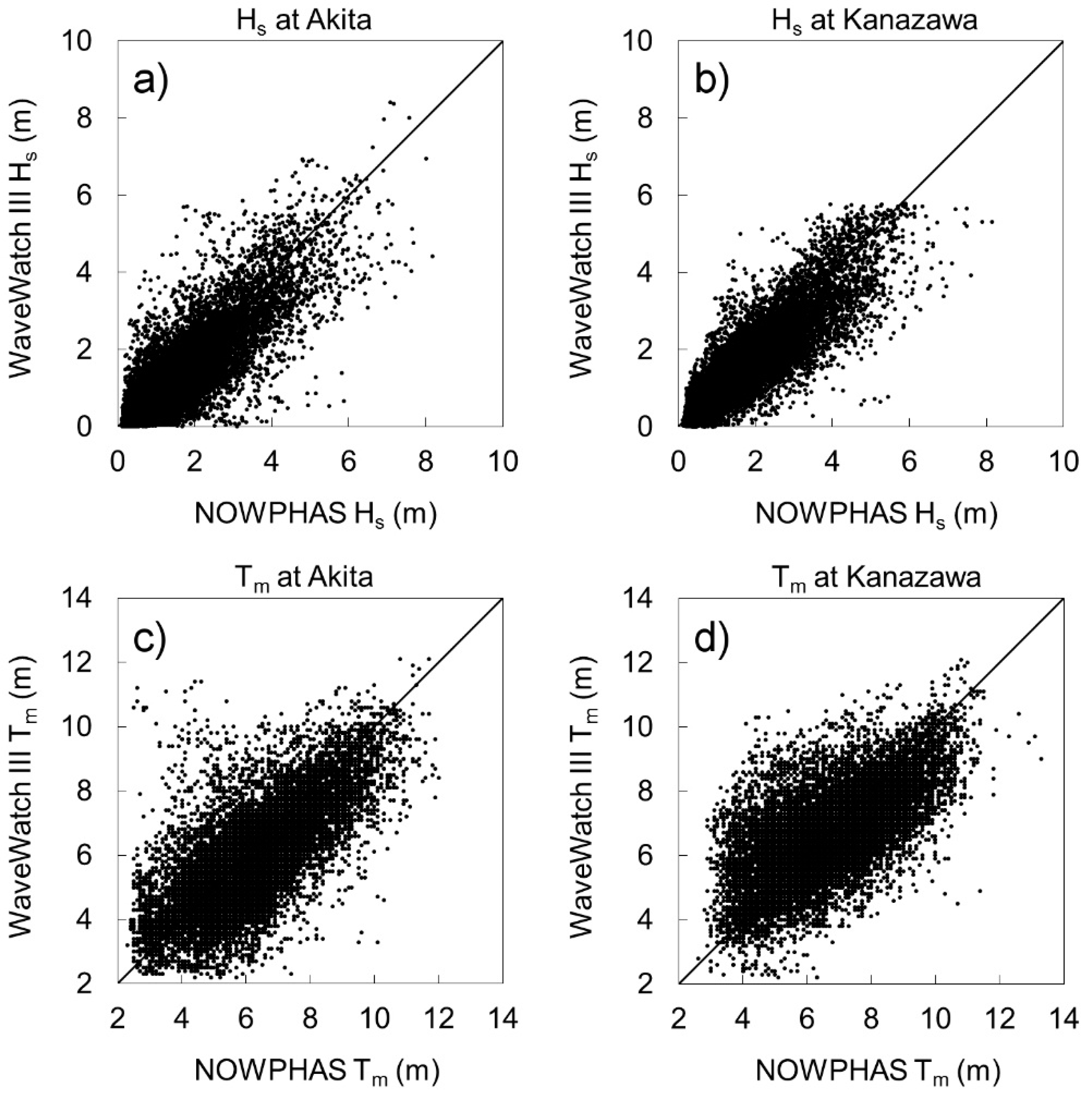
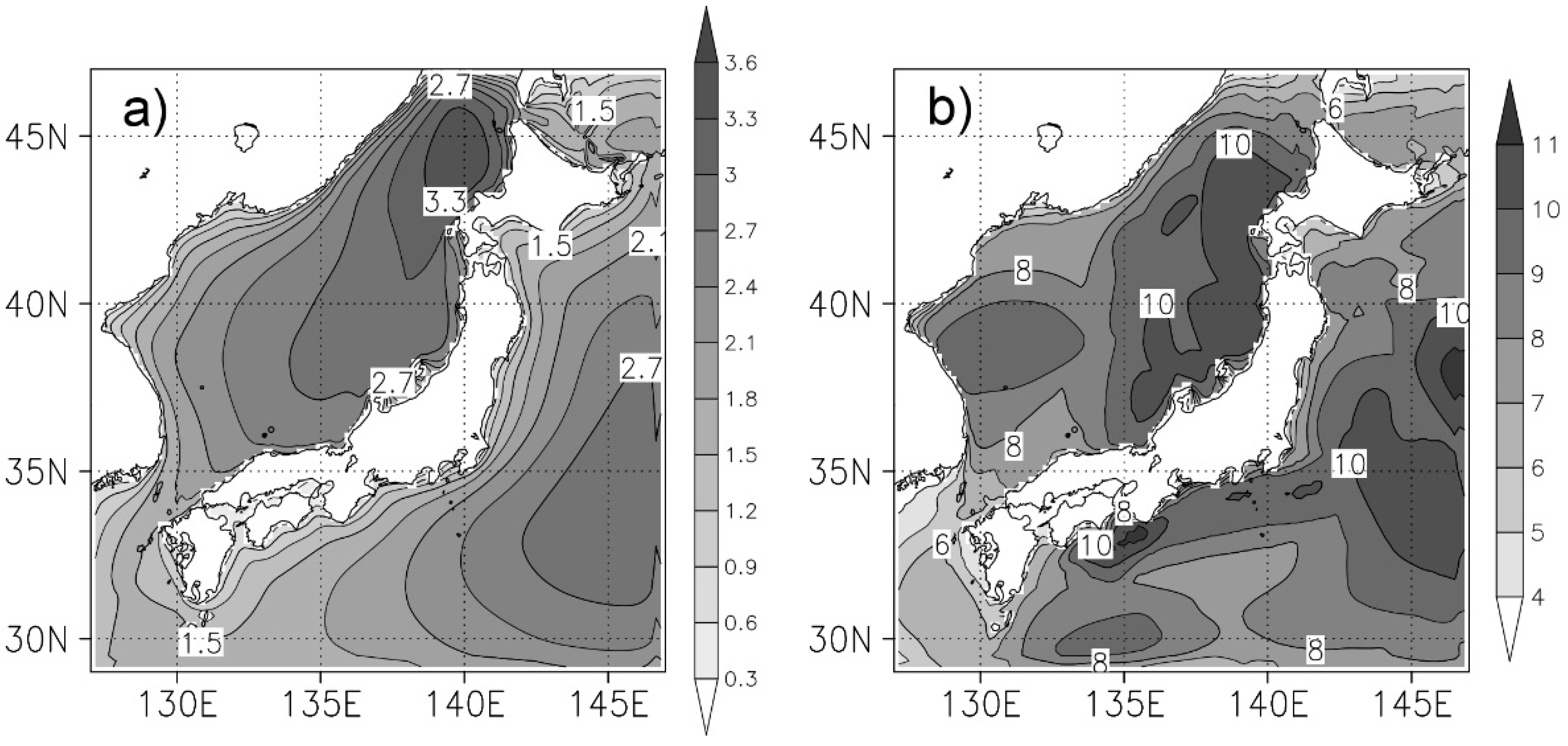
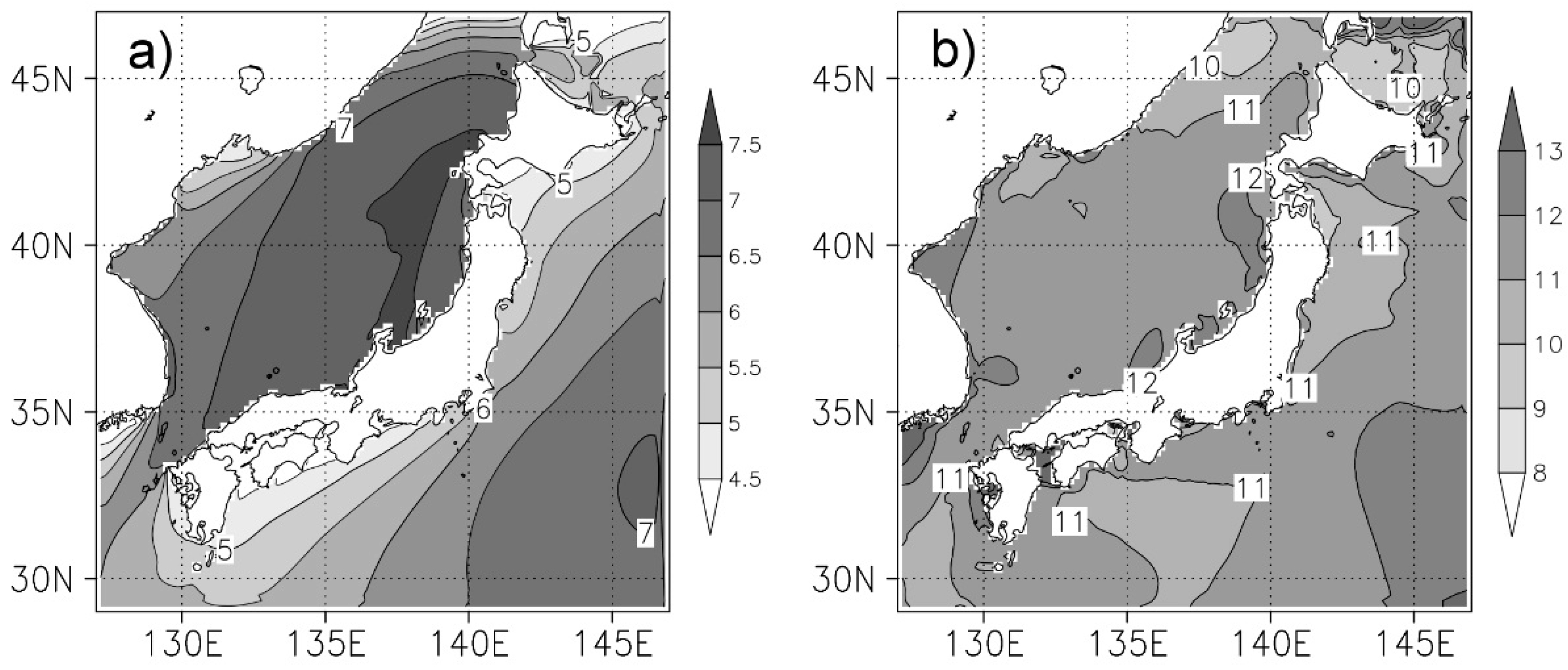
3.1. Validation of Present Wave Climate Simulated by WW3

The results of the wave simulation with historical forcing were validated with NOWPHAS observational data from Akita and Kanazawa. The historical wave simulations were made for 11 years but the comparison data were obtained during 2001–2010 because of NOWPHAS limitations. The output interval of the wave simulations was 1 h but the interval of NOWPHAS observations is 2 h. Therefore, the simulated wave characteristics were examined for the target periods (5 months from October to February in target years) with 2-hourly data (more than 16,000 data for the simulations and the observations). Figure 2 shows comparisons of significant wave height (H_s) and mean wave period (T_m) at the two observation sites. Significant wave height shows some scattering but no significant bias at either site. The correlation coefficient for Akita and Kanazawa is 0.83 and 0.86, respectively. At Akita, the maximum value of H_s is >8.0 m for both the simulation and the observation data. However, the simulated maximum H_s is about 6.0 m at Kanazawa, whereas the observed maximum H_s is >8.0 m. Thus, high waves are slightly underestimated by WW3 at Kanazawa. The mean wave period varies more widely than H_s and the correlation coefficient is 0.70 and 0.64 for Akita and Kanazawa, respectively. However, there is no significant bias in T_m. These results indicate good agreement between the simulated and the observed wave climates.

Figure 3 shows the spatial distributions of climatological significant wave height (${\overline{H}}_s$) and maximum significant wave height (H_{s_max}) in winter (December–February: DJF) in the parent domain during the target period for the wave simulation. Over a wide area of the Japan Sea side, ${\overline{H}}_s$ along the coast is >2.1 m, whereas it is smaller (~0.9 m) along the coast on the Pacific side. In winter, strong northwesterly winds that blow over the Japan Sea cause higher ocean waves. Therefore, H_{s_max} in winter is >10 m over the northern half of the coastal area on the Japan Sea side, whereas it is >10 m near only a limited area of the coast on the Pacific side.

Figure 4 illustrates the spatial distributions of climatological mean wave period (${\overline{T}}_m$) and maximum mean wave period (T_{m_max}) in DJF during the target period. On the Japan Sea side, waves with ${\overline{T}}_m$ > 7 s reach the coast. On the Pacific side, waves with ${\overline{T}}_m$ of 5.0–5.5 s are found over a wide area. There are some differences between the spatial patterns of ${\overline{T}}_m$ and ${\overline{H}}_s$ but the same tendencies (ocean waves are larger on the Japan Sea side) can be recognized within them. The values of T_{m_max} in CTL are comparable between the Japan Sea side and the Pacific side. However, there are clear differences between the spatial patterns of T_{m_max} and H_{s_max} in CTL.

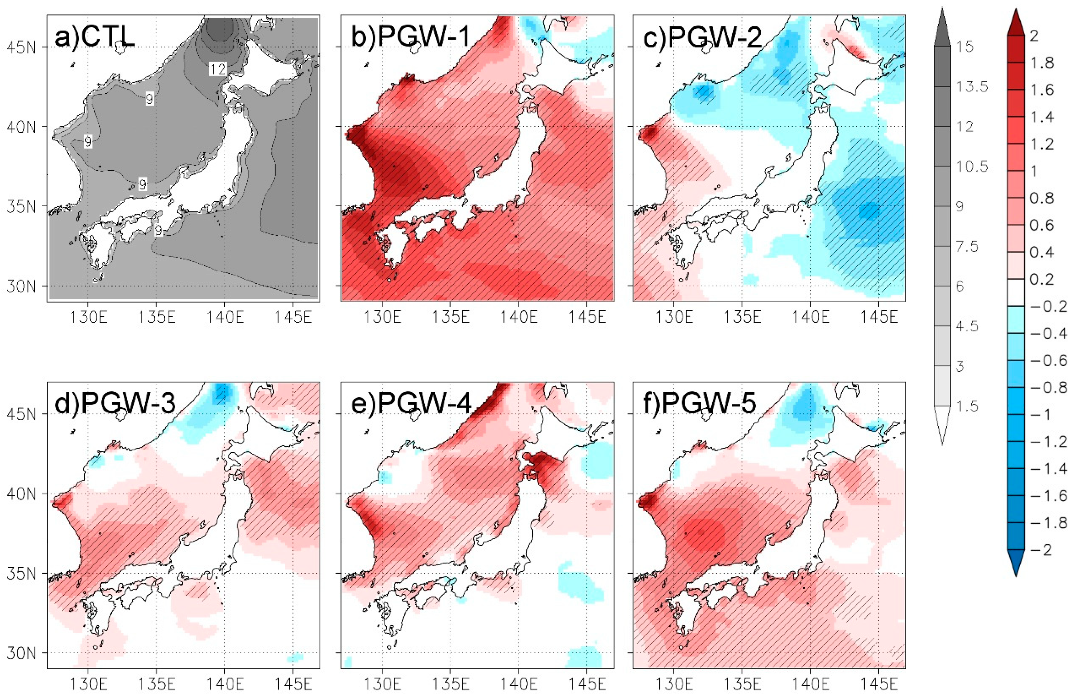
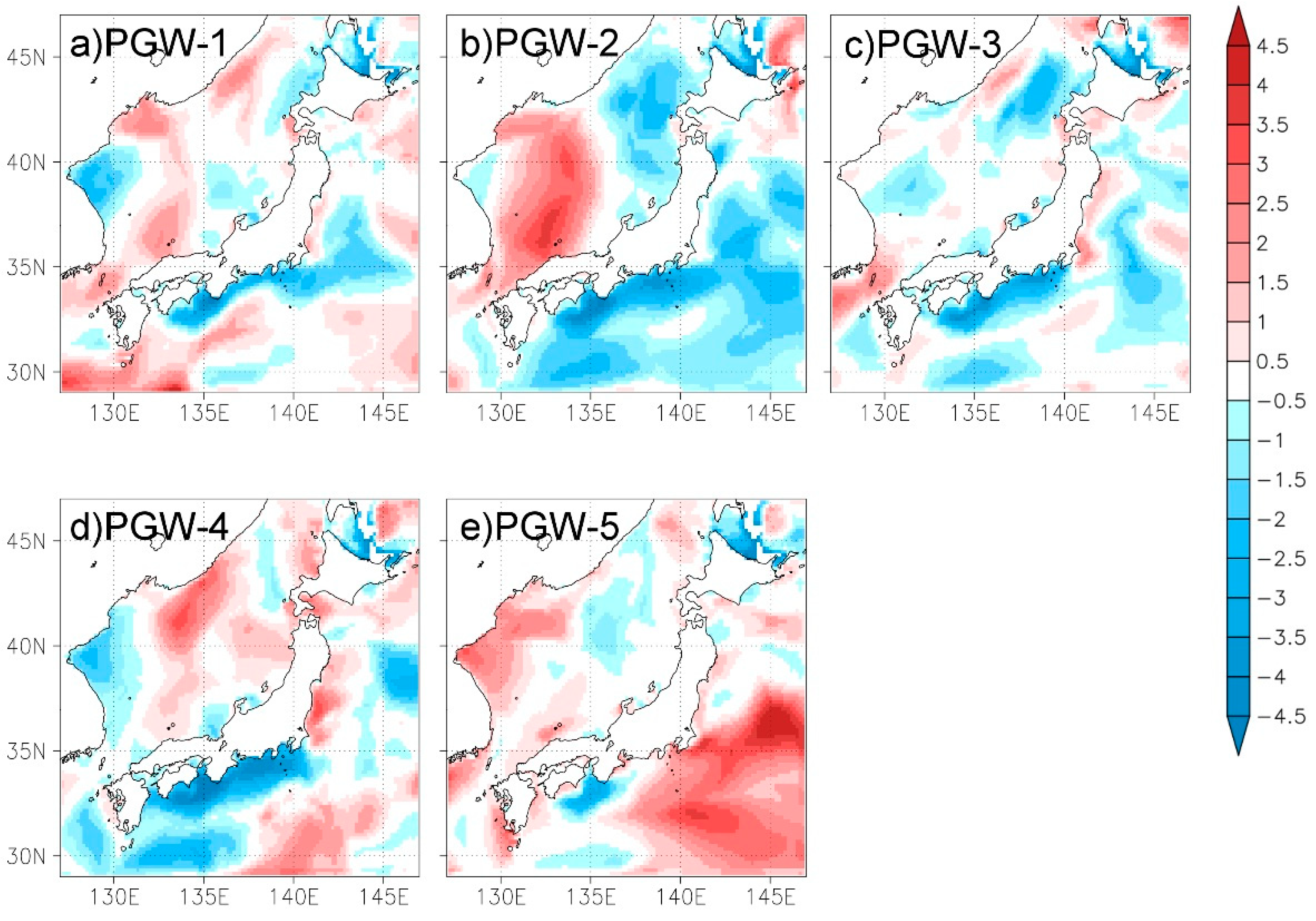
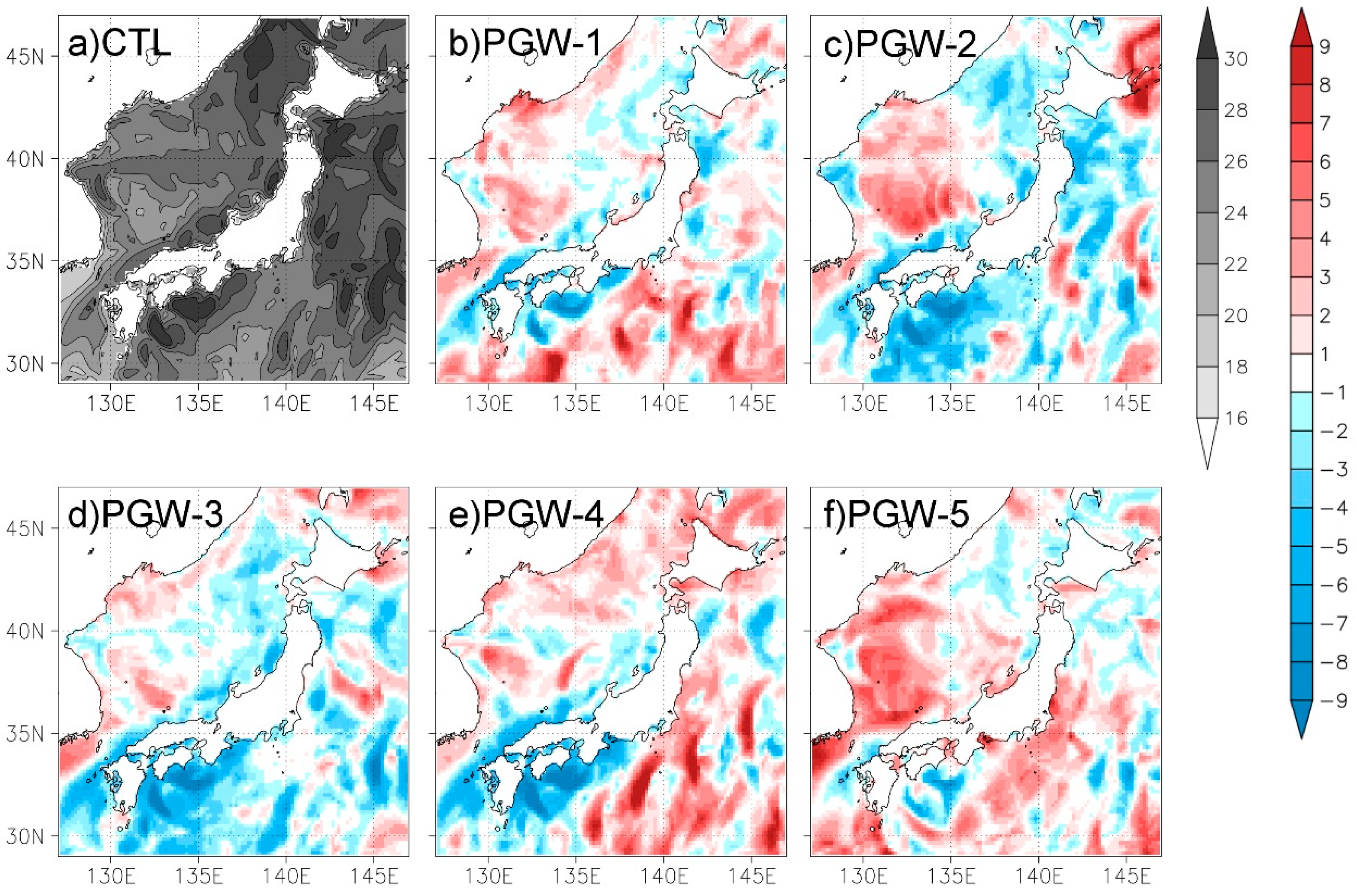
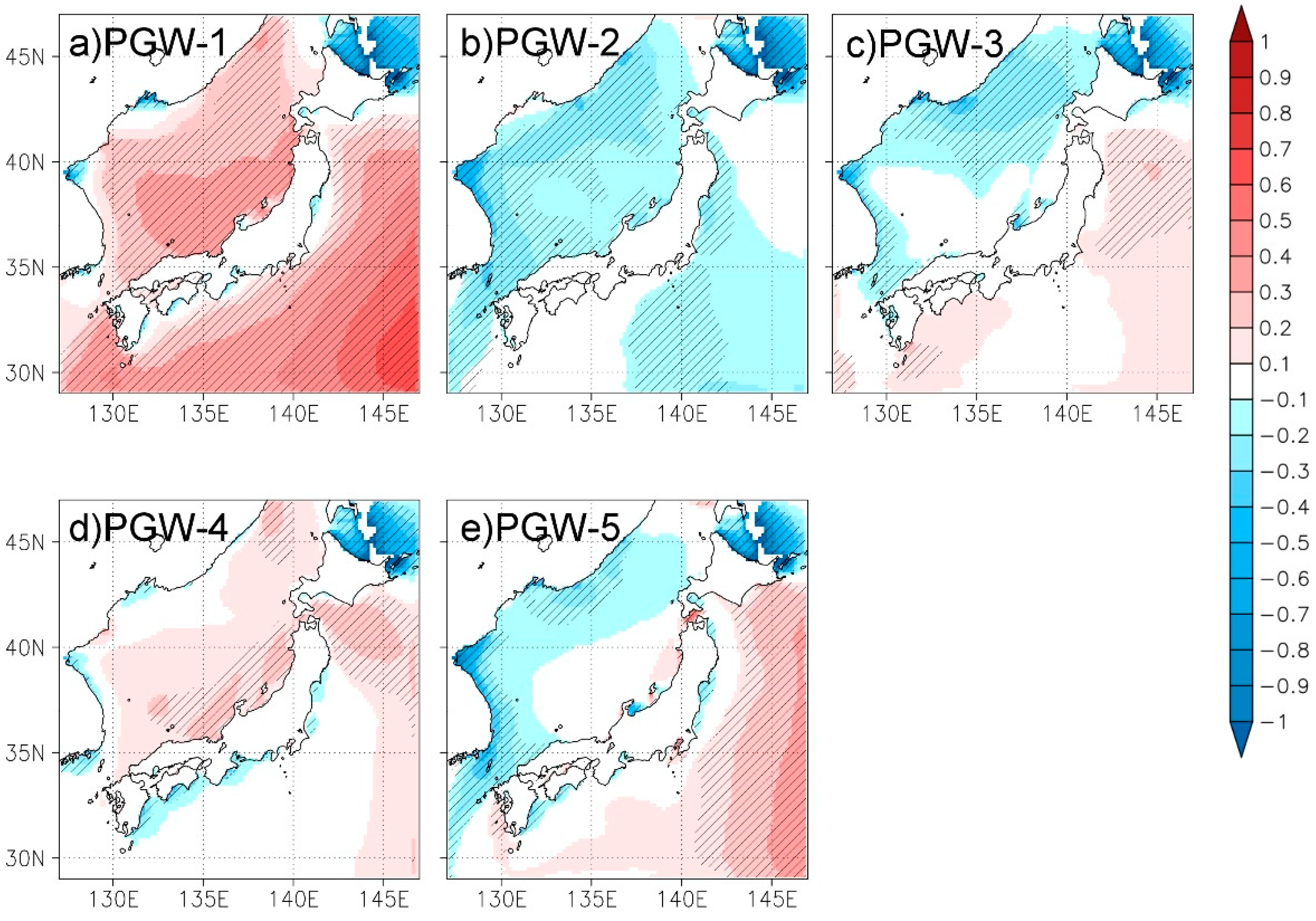
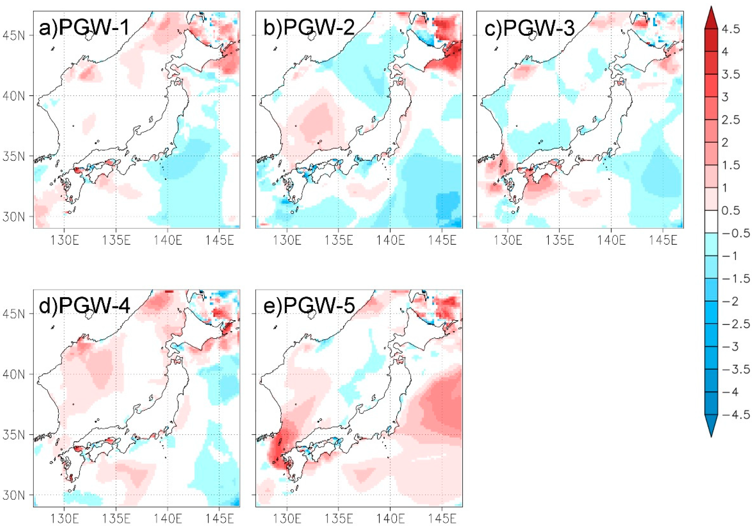
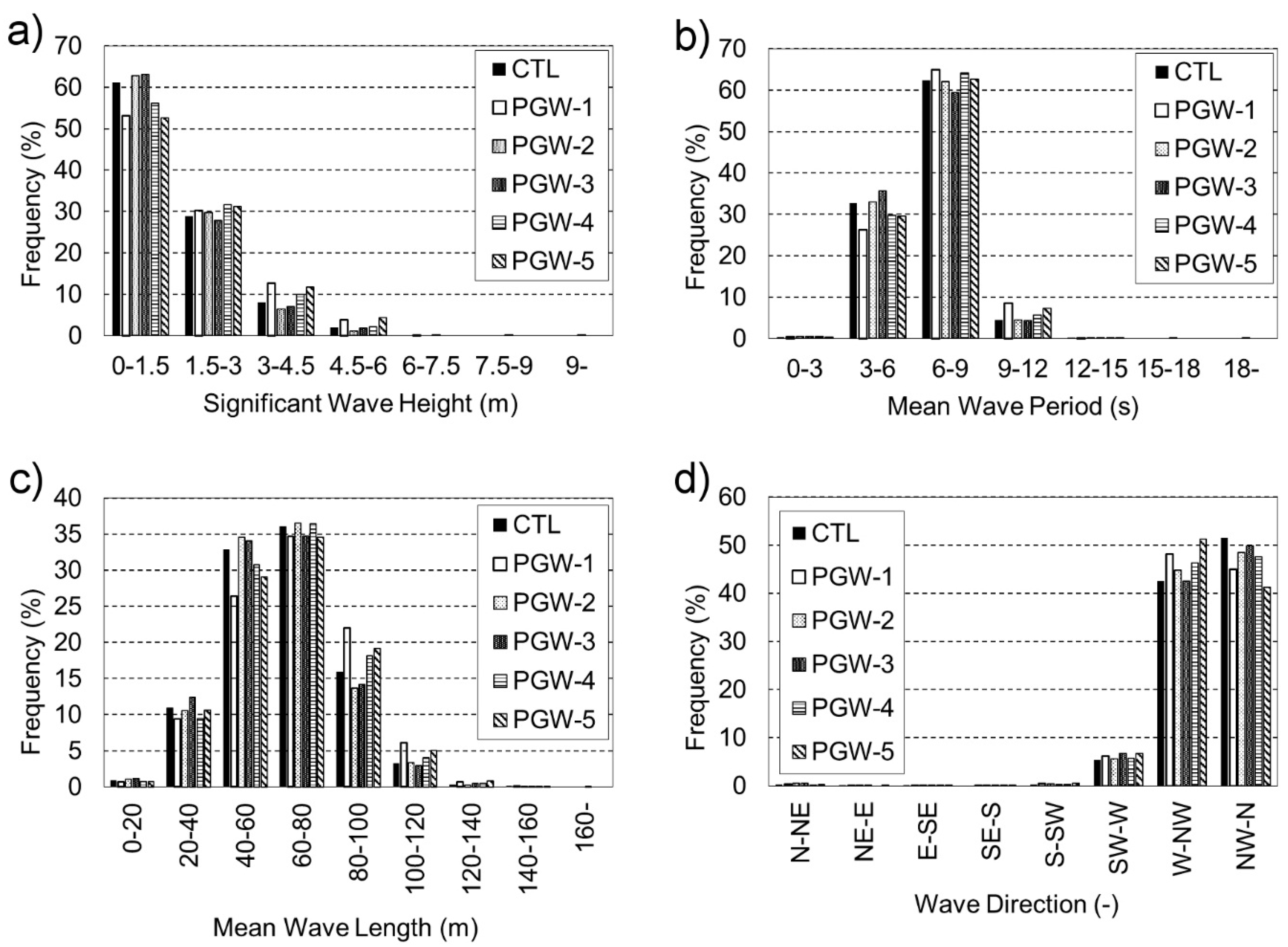
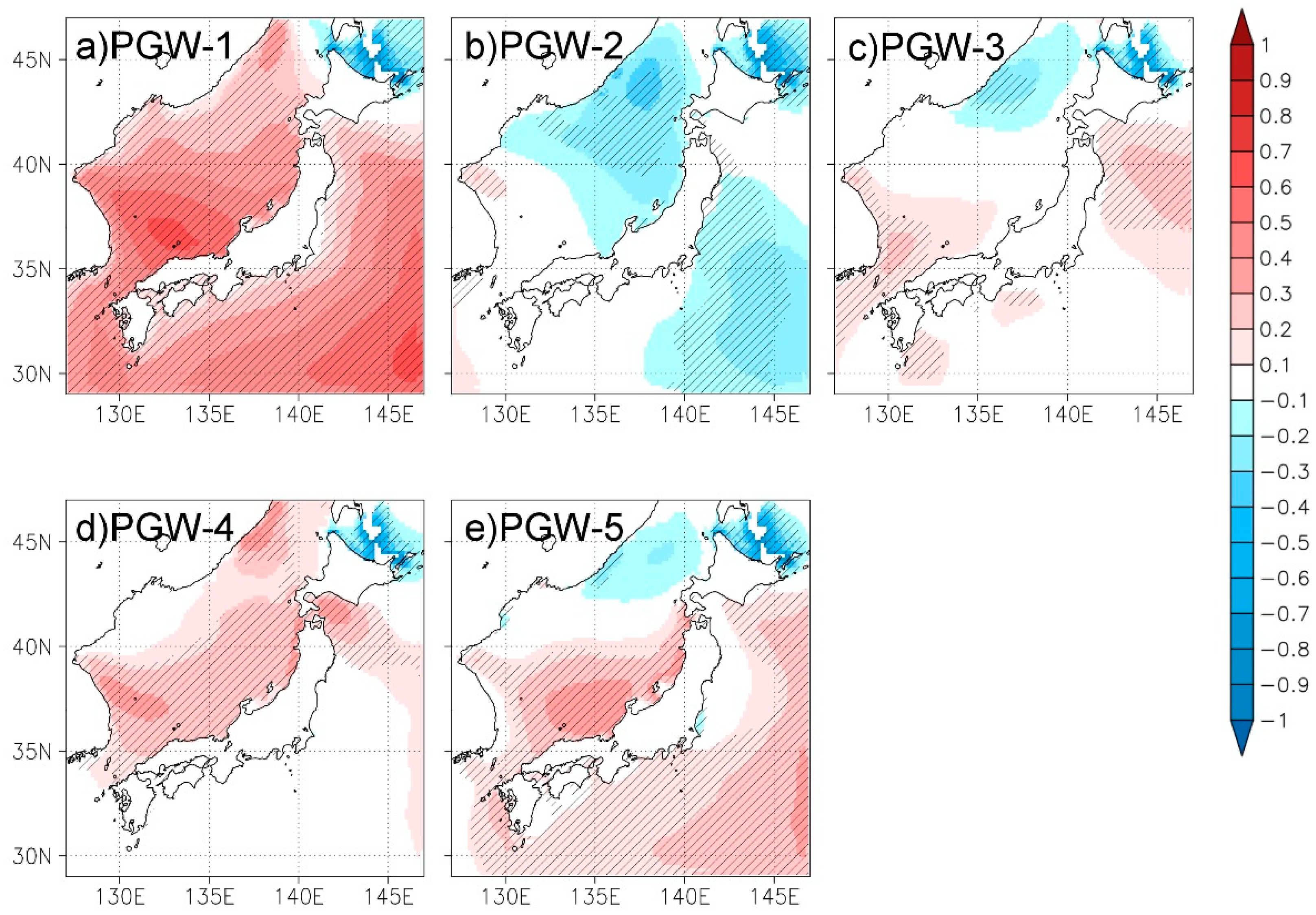
3.2. Future Variations of Wave Characteristics around Japan

The Japan Sea is rather enclosed and its wave characteristics are affected largely by the wind climate over the Japan Sea. Figure 5 shows the climatological mean wind speed in winter (DJF) and its future variations. Here, Welch’s t-test [24] was applied to examine the significance of difference between the climatological mean wind speed in present and in future climate. CTL shows that mean wind speed at 10 m above the sea surface (${\overline{U}}_{10}$) is 9 m/s or more around Japan during winter. In PGW-1, 3, 4, and 5 increasing tendencies of ${\overline{U}}_{10}$ can be seen over the Japan Sea, and these tendencies are statistically significant in wide areas. Although PGW-2 shows a decreasing or small variation over the Japan Sea, it is not statistically significant along the coast. These results indicate the high likelihood of an increasing tendency of ${\overline{H}}_s$ in winter over the Japan Sea. On the Pacific side, widespread significant changes of ${\overline{U}}_{10}$ are found only in two PGW runs (i.e., PGW-1 and 5), and there are larger uncertainties of ${\overline{U}}_{10}$ in the Pacific.

Figure 6 shows the differences in ${\overline{H}}_s$ in winter between the future and present climates. In PGW-1, ${\overline{H}}_s$ is larger than in the present climate over a wide area of the parent domain. Almost all the increasing tendencies are statistically significant. The results of PGW-5 also show a statistically significant increase in ${\overline{H}}_s$ over wide areas. Larger values of ${\overline{H}}_s$ in the future are also found in PGW-4 but mainly on the Japan Sea side. In PGW-3, an increasing tendency of ${\overline{H}}_s$ is recognized around Japan, whereas no significant increase is evident on the Japan Sea side. Conversely, PGW-2 shows the opposite tendency, but without any statistically significant variation in the coastal area on the Japan Sea side. The patterns of ${\overline{H}}_s$ variation are similar to ${\overline{U}}_{10}$, which indicate the climatology of ${\overline{H}}_s$ is controlled primarily by ${\overline{U}}_{10}$.

Figure 7 shows the variations of H_{s_max} in the future climate. On the Pacific side, all PGW simulations show decreasing H_{s_max} along the southern parts of the coast (south of 35° N), and four PGW simulations (except PGW-2) show slight increasing tendencies in northern parts. On the Japan Sea side, H_{s_max} increases somewhat to the west of 135° E, but to the east of this longitude, no common characteristics are evident in the variation of H_{s_max} in the future climate. Figure 8 shows the maximum wind speed in winter ($U_{10\_max}$) for CTL, and its differences between CTL and each PGW run. On the Pacific side, the patterns of future variation of $U_{10\_max}$ and H_{s_max} show some similarities in each of the PGW simulations. However, decreasing $U_{10\_max}$ is found to the west of 136° E on the Japan Sea side, whereas increasing H_{s_max} is found in PGW-1, 2, 4, and 5. This result indicates H_{s_max} in the west of the Japan Sea side is affected not only by local but also by remote wind conditions. In the eastern part of the Japan Sea side, as seen in H_{s_max}, $U_{10\_max}$ does not show any common tendency between the five PGW simulations. These results indicate H_{s_max} is only somewhat affected by $U_{10\_max}$.

Figure 9 shows differences of ${\overline{T}}_m$ between CTL and each PGW run during winter. The results of PGW-1 and 4 show statistically significant increasing trends along the coast of the Japan Sea. A decreasing wave period is recognized in PGW-2, except for the northern part of the Japan Sea side. Neither PGW-3 nor 5 show significant variations of ${\overline{T}}_m$ on the Japan Sea side. On the Pacific side, PGW-1 shows a significant increase but the opposite result is found in PGW-2. In the other three PGW runs, there are no clear variations on the Pacific side. The patterns of future variation of ${\overline{T}}_m$ and ${\overline{U}}_{10}$ show some similarities in PGW-1, and 4, but certain differences in PGW-2, 3, and 5. These results indicate ${\overline{T}}_m$ is affected less by ${\overline{U}}_{10}$ than ${\overline{H}}_s$. Figure 10 shows the results of the maximum wave period (T_{m_max}). All of the five PGW simulations show different patterns of future variation of T_{m_max}, making it difficult to discern any common characteristics. In comparison with future variations of $U_{10\_max}$ (Figure 8), PGW-2 does show some similarity, but the patterns of future variations of $U_{10\_max}$ and T_{m_max} are clearly different in the other four PGW runs. The results in Figure 9 and Figure 10 do not show robust relationship between the wave period and wind speed. It indicates that statistical approaches fail to estimate future variations in wave period by using wind speed, but numerical wave simulations are indispensable.

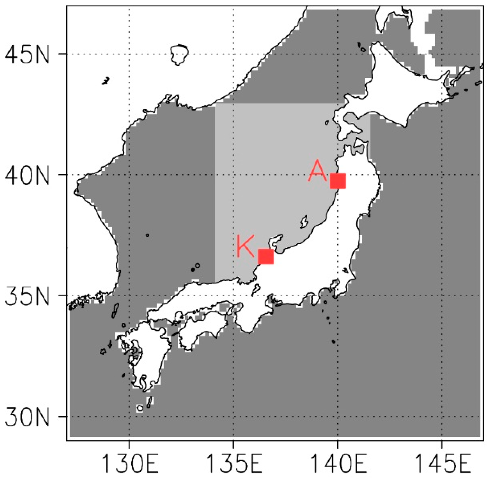
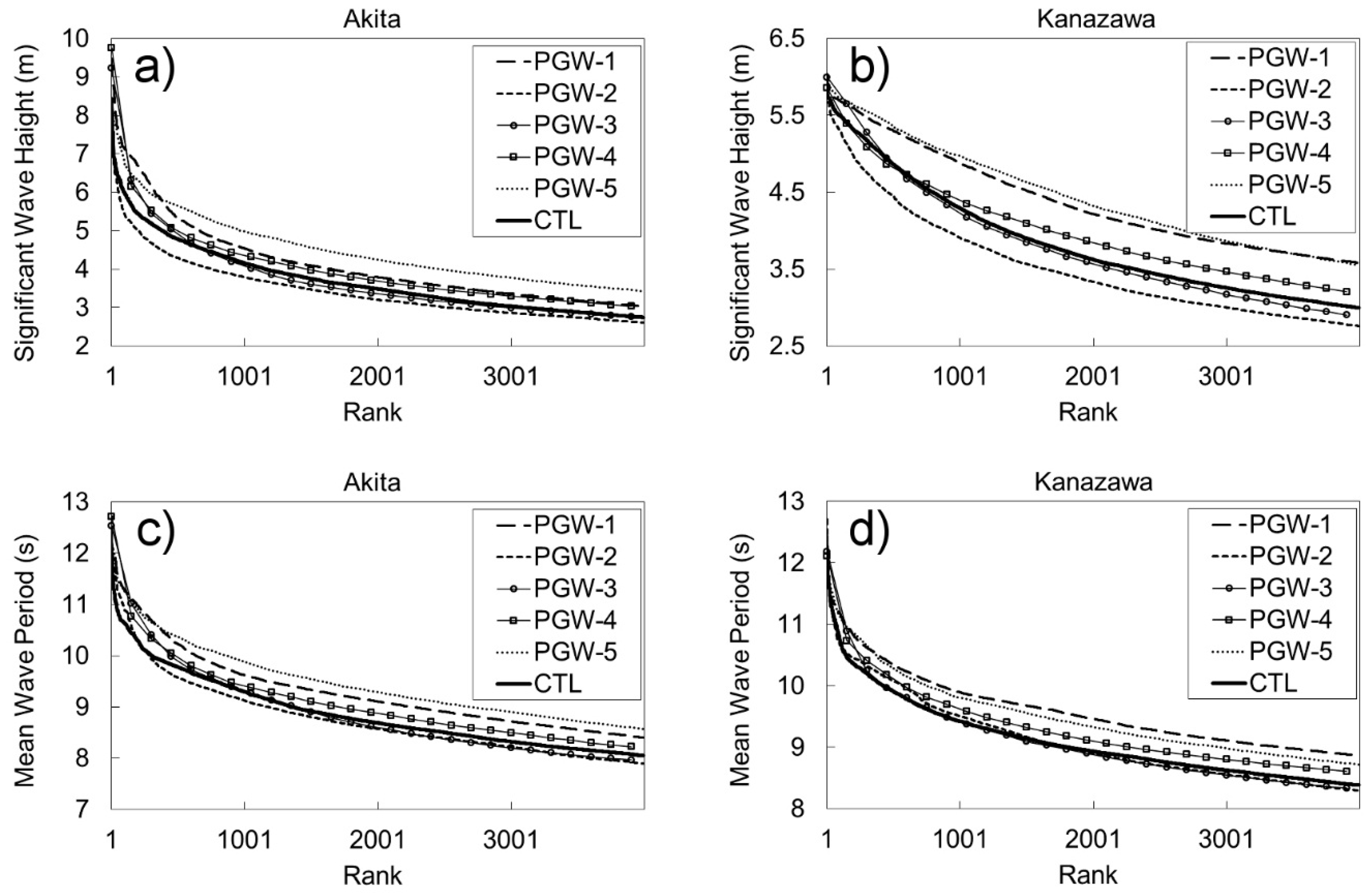
3.3. Details of Future Variations of Wave Characteristics at Kanazawa and Akita

Details of the future variations of wave characteristics at Kanazawa and Akita were investigated. Figure 11 shows the top 1% (about 4000 values) of H_s and T_m at the two sites. The results of PGW-2 show the top 1% of H_s is smaller than CTL at both sites. For T_m, the results of PGW-2 are slightly smaller than CTL at Akita but comparable at Kanazawa. PGW-3 shows that H_s and T_m are comparable with CTL at both Akita and Kanazawa. The results of PGW-1, 4, and 5 show the top 1% of H_s and T_m are larger than CTL. Figure 7 and Figure 10 do not show any significant or common features in future variations of H_{s_max} and T_{m_max}. However, Figure 11 does show larger ocean waves affect the coast on the Japan Sea side more frequently in more than half of the PGW simulations. This might not cause severe damage but it could change the coastal environment.

Figure 12 presents the frequency distributions of the wave climate at Akita. The higher class of values of wave characteristics was investigated in Figure 11, whereas variations in the lower class of values are the focus here. The results of H_s show small variations in PGW-2 and 3, but the other three future simulations show an increasing frequency in H_s > 1.5–3.0 m and a decreasing frequency in H_s of 0.0–1.5 m. The results of T_m show an increasing frequency of waves with periods >6 s and a decreasing frequency of waves with periods <6 s in PGW-1, 4, and 5. In Figure 9, PGW-2 does not show an increasing tendency of ${\overline{T}}_m$, whereas Figure 12 does show a slight increase in T_m of 6–9 s at Akita. Frequency distributions of significant wavelength show smaller variations in PGW-3. The results of PGW-1 and 5 show a clear decrease in waves with wavelengths <60 m and a significant increase in waves with longer wavelengths. PGW-2 and 4 also show a decrease in shorter wavelengths and an increase in longer wavelengths but the variations are smaller than PGW-1 and 5. Wave directions also show some differences in the future. PGW-1 and PGW-5 show a clear increase in ocean waves from the SW–W and a decrease in waves from the S–SW and W–NW. It indicates that waves from the west will increase in future at Akita. However, the other three PGW runs do not present any common characteristics.

Figure 13 is the same as Figure 12 but for Kanazawa. An increasing frequency of higher values of H_s is evident in PGW-1, 4, and 5, whereas PGW-2 and 3 show a small increase in smaller values of H_s (0.0–1.5 m). PGW-2 shows an increase in H_s of 1.5–3.0 m but a decrease in larger H_s in the future. The results of T_m show an increase in longer period waves in PGW-1, 4, 5, and an increase in shorter period waves (3–6 s) in PGW-3. There are small variations of T_m in PGW-2. The results of wavelength show similar tendencies to T_m (Figure 13c). Wave directions show similar tendencies in future variation among the five PGW simulations at Kanazawa. The frequency of waves from the NW–N decreases in the five PGW runs, whereas waves from W–NW increase in frequency in PGW-1, 2, 4, and 5. In PGW-3, waves from SW–W increase slightly in the future. These results indicate the high probability of an increase in the frequency of waves from the west in the future at Kanazawa.

It is indicated that, as well as the extreme wave climate, the daily wave climate is also important [5]. Ocean waves with small values of H_s do not affect the coastal environment over short periods, but the accumulated effects of changes in the wave climate might have an impact on coastal areas. Figure 11 shows that, although not extreme, relatively higher waves will occur more frequently in the future. Figure 5, Figure 12, and Figure 13 all indicate that the daily H_s will be greater in the future climate modeled in PGW-1, 4, and 5. Based on this analysis, the impacts of changes in wave climate should be discussed. Furthermore, it is recognized that detailed simulations are indispensable for planning, design, and assessment in relation to coastal environments.

4. Conclusions

Using a third-generation wave model, the winter wave climate of the Japan Sea was projected based on five different GCM products. Sea surface wind speed, which was used for forcing the wave simulation, showed significant enhancement in the Japan Sea under the condition of global warming in four out of five future projections. Corresponding to the enhanced wind, the mean significant wave height over the Japan Sea is projected to become greater in the future climate. In one future projection (PGW-2), clear variations were not recognized in sea surface wind and mean significant wave height along the coast of the Japan Sea. The mean wave period did not show any common tendency in the five future projections. The maxima of significant wave height and of mean wave period also did not show clear future variations in the Japan Sea. The top 1% of significant wave heights and mean wave periods indicated higher and longer wavelength ocean waves in more than half of the future projections. In two future projections (PGW-2 and PGW-3), top 1% significant wave height and mean wave period are comparable to or smaller than in the present climate. The frequency distributions of significant wave height, mean wave period, mean wave length, and wave direction showed a range of different variations among the five future projections. Significant wave height showed a certain shift in several future projections. These results indicate that, although not extreme, the daily significant wave height will become greater along the coast of the Japan Sea. The frequency distributions of the mean wave period and wavelength also indicated that daily ocean waves would become longer. The results of wave directions showed an increasing frequency of waves from the west in four projections at Kanazawa. Daily ocean waves cannot cause severe disasters or change the topography and environment of the coast over short periods. However, the repetitive effect of ocean waves could have certain impact on coastal areas over the long term. Therefore, changes in daily ocean climate cannot be neglected, and long-term simulations of coastal morphology or the coastal environment are recognized as indispensable in assessing future variations and for preparing adaptation strategies.

Some future variations are common among more than half the multiple projections using different GCMs, but there are uncertainties that remain in the results of the wave simulations. For example, in the northern part of the Japan Sea showed an opposite tendency of variation (Figure 6), i.e., both increasing and decreasing tendencies were statistically significant in that area. In [16], a statistical downscaling method was applied using multiple GCM projections to estimate global wave height and sea level rise, and opposite (i.e., increasing and decreasing) trends of H_s were found in different regions. At the same time, large uncertainties in the projected values of H_s for different GCMs were also reported. Ocean waves are controlled by local/remote sea surface winds, but the projections of GCMs and the outputs of weather forecasting models are not perfect. In this moment, it is difficult to elicit definitive conclusions of future variations of wave climate along the coast of the Japan Sea. But, in order to exploit available future projections, a probabilistic evaluation method should be established using multiple model outputs. Furthermore, bias correction of the forcing data could be a useful method to prevent some of the uncertainties. To utilize future projections based on multiple global experiments, the development of postprocessing techniques or methods for interpretation will be indispensable.

Numerical wave simulations can provide wave spectra. In this study, changes in H_s and T_m were examined, but from a scientific point of view, the reasons behind the changes in wave climate are of greater interest. Using wave spectra, the causes of the changes in wave characteristics (e.g., effects of local wind waves or remotely developed swell) could be investigated. This would enable an assessment of their impact and further the understanding of the mechanism of variations in wave climate, which is an important challenge in this field.

References

1. Wang, X.L.; Swail, V.R. Climate change signal and uncertainty in projections of ocean wave height. Clim. Dyn. 2006, 26, 109–126. [Google Scholar] [CrossRef]
2. Wang, X.L.; Feng, Y.; Swail, V.R. Changes in global ocean wave heights as projected using multi-model CMIP5 simulations. Geophys. Res. Lett. 2014, 41, 1026–1034. [Google Scholar] [CrossRef]
3. Taylor, K.E.; Stouffer, R.K.; Meehl, G.A. An overview of CMIP5 and the experiment design. Bull. Am. Meteorol. Soc. 2012, 93, 485–498. [Google Scholar] [CrossRef]
4. Perez, J.; Menendez, M.; Camus, P.; Mendez, F.J.; Losada, I.J. Statistical multi-model climate projections of surface ocean waves in Europe. Ocean Model. 2015, 96, 161–170. [Google Scholar] [CrossRef]
5. Mori, N.; Yasuda, T.; Mase, H.; Tom, T.; Oku, Y. Projection of extreme wave climate change under global warming. Hydrol. Res. Lett. 2010, 4, 15–19. [Google Scholar] [CrossRef]
6. Charles, E.; Idier, D.; Delecluse, P.; Déqué, M.; Le Cozannet, G. Climate change impact on waves in the Bay of Biscay, France. Ocean Dyn. 2012, 62, 831–848. [Google Scholar] [CrossRef]
7. Groll, N.; Grabemann, I.; Gaslikova, L. North Sea wave conditions: An analysis of four transient future realizations. Ocean Dyn. 2014, 64, 1–12. [Google Scholar] [CrossRef]
8. Grabemann, I.; Groll, N.; Möller, J.; Weisse, R. Climate change impact on North Sea wave conditions: A consistent analysis of ten projections. Ocean Dyn. 2015, 65, 255–267. [Google Scholar] [CrossRef]
9. Hemer, M.A.; Katzfey, J.; Trenham, C.E. Global dynamical projections of surface ocean wave climate for a future high green gas emission scenario. Ocean Model. 2013, 70, 221–245. [Google Scholar] [CrossRef]
10. Semedo, A.; Weisse, R.; Behrens, A.; Sterl, A.; Bengtsson, L.; Günter, H. Projection of global wave climate change toward the end of the twenty-first century. J. Clim. 2013, 26, 8269–8288. [Google Scholar] [CrossRef]
11. Fan, Y.; Lin, S.-J.; Griffies, S.M.; Hemer, M.A. Simulated global swell and wind-sea climate and their response to anthropogenic climate change at the end of the twenty-first century. J. Clim. 2014, 27, 3516–3536. [Google Scholar] [CrossRef]
12. Erikson, L.H.; Hegermiller, C.A.; Barnard, P.L.; Ruggiero, P.; van Ormondt, M. Projected wave conditions in the Eastern North Pacific under the influence of two CMIP5 climate scenarios. Ocean Model. 2015, 96, 171–185. [Google Scholar] [CrossRef]
13. Shimura, T.; Mori, N.; Mase, H. Future projection of ocean wave climate: Analysis of SST impacts on wave climate change in the western North Pacific. J. Clim. 2015, 28, 3171–3190. [Google Scholar] [CrossRef]
14. Laugel, A.; Menendez, M.; Benoit, M.; Mattarolo, G.; Méndez, F. Wave climate projections along the French coastline: Dynamical versus statistical downscaling. Ocean Model. 2014, 84, 35–50. [Google Scholar] [CrossRef]
15. Martínez-Asensio, A.; Marcos, M.; Tsimplis, M.N.; Jordà, G.; Feng, X.; Gomis, D. On the ability of wind-wave models to capture the variability and long-term trends of the North Atlantic winter wave climate. Ocean Model. 2016, 103, 177–189. [Google Scholar] [CrossRef]
16. Mori, N.; Shimura, T.; Yasuda, T.; Mase, H. Multi-model climate projections of ocean surface variables under different climate scenarios—Future change of waves, sea level and wind. Ocean Eng. 2013, 71, 122–129. [Google Scholar] [CrossRef]
17. Hemer, M.A.; Trenham, C.E. Evaluation of a CMIP5 derived dynamical global wind wave climate model ensemble. Ocean Model. 2016, 103, 190–203. [Google Scholar] [CrossRef]
18. Sato, T.; Kimura, F.; Kitoh, A. Projection of global warming onto regional precipitation over Mongolia using a regional climate model. J. Hydrol. 2007, 333, 144–154. [Google Scholar] [CrossRef]
19. Taniguchi, K. Future changes in precipitation and water resources for Kanto Region in Japan after application of pseudo global warming method and dynamical downscaling. J. Hydrol. Reg. Stud. 2016, 8, 287–303. [Google Scholar] [CrossRef]
20. Skamarock, W.C.; Klemp, J.B.; Dudhia, J.; Gill, D.O.; Barker, D.M.; Duda, M.G.; Huang, X.-Y.; Wang, W.; Powers, J.G. A description of the advancedresearch WRF version 3. NCAR. Tech. Note NCAR/TN-475 + STR 2008, 113. [Google Scholar] [CrossRef]
21. Onogi, K.; Tsutsui, J.; Koide, H.; Sakamoto, M.; Kobayashi, S.; Hatsushika, H.; Matsumoto, T.; Yamazaki, N.; Kamahori, H.; Takahashi, K.; et al. The JRA-25 Reanalysis. J. Meteorol. Soc. Jpn. 2007, 85, 369–432. [Google Scholar] [CrossRef]
22. Tolman, H.L. User manual and system documentation of WaveWatch III version 3.14. Tech. Note MMAB Contrib. 2009, 276, 220. [Google Scholar]
23. Tolman, H.L.; Chalikov, D.V. Source term in a third-generation wind-wave model. J. Phys. Oceanogr. 1996, 26, 2497–2518. [Google Scholar] [CrossRef]
24. Welch, B.L. The significance of the difference between two means when the population variances are unequal. Biometrika 1938, 29, 350–362. [Google Scholar] [CrossRef]
Figure 1. Target domains of the wave simulation. Darker region is the parent domain and brighter region is the child domain. The Nationwide Ocean Wave information network for Ports and HArbourS (NOWPHAS) observation sites at Akita and Kanazawa are indicated by red squares with initials A and K, respectively.
Jmse 07 00150 g001
Figure 2. Significant wave height (Hs) and mean wave period (Tm) by NOWPHAS observation and WaveWatchIII (WW3) simulation. (a) Hs at Akita, (b) Hs at Kanazawa, (c) Tm at Akita, and (d) Tm at Kanazawa. Horizontal and vertical axes of each panel represent NOWPHAS and WW3, respectively.
Jmse 07 00150 g002
Figure 3. Results of Hs for historical wave simulation by WW3. (a) Climatological mean Hs ( H ¯ s ) for December–February (DJF) and (b) maximum Hs (Hs_max) during the target period (2000–2010). Unit of color bars is m.
Jmse 07 00150 g003
Figure 4. Results of Tm for historical wave simulation by WW3. (a) Climatological mean Tm ( T ¯ m ) for DJF and (b) maximum Tm (Tm_max) during the target period (2000–2010). Unit of color bars is s.
Jmse 07 00150 g004
Figure 5. Spatial distribution of mean wind speed. (a) Climatological mean winter wind speed ( U ¯ 10 ) of CTL, and (b)–(f) future variations of U ¯ 10 in each PGW simulation. Left-hand color bar is for U ¯ 10 in CTL and right-hand color bar is for future variations of U ¯ 10 . Unit of color bars is m/s. Areas with statistically significant variation are indicated by hatching.
Jmse 07 00150 g005
Figure 6. (a)–(e) Future variations of H ¯ s in each PGW simulation. Areas with statistically significant variation are indicated by hatching. Unit of color bar is m.
Jmse 07 00150 g006
Figure 7. (a)–(e) Future variations of Hs_max in each PGW simulation. Unit of color bar is m.
Jmse 07 00150 g007
Figure 8. Spatial distribution of maximum wind speed ( U 10 _ m a x ) in the target period. (a) U 10 _ m a x in CTL, and (b)–(f) future variations of U 10 _ m a x in each PGW simulation. Left-hand color bar is for U 10 _ m a x in CTL and right-hand color bar is for future variations of U 10 _ m a x . Unit of color bars is m/s.
Jmse 07 00150 g008
Figure 9. (a)–(e) Future variations of T ¯ m in each PGW simulation. Areas with statistically significant variation are indicated by hatching. Unit of color bar is sec.
Jmse 07 00150 g009
Figure 10. (a)–(e) Future variations of Tm_max in each PGW simulation. Unit of color bar is sec.
Jmse 07 00150 g010
Figure 11. Top 1% (about top 4000) of Hs and Tm at Akita and Kanazawa. (a) Hs at Akita, (b) Hs at Kanazawa, (c) Tm at Akita, and (d) Tm at Kanazawa. Horizontal axis is rank and vertical axis is Hs for (a) and (b), and Tm for (c) and (d).
Jmse 07 00150 g011
Figure 12. Frequency distribution of wave characteristics at Akita. (a) Hs, (b) Tm, (c) mean wavelength, and (d) wave direction. Frequencies are shown in %.
Jmse 07 00150 g012
Figure 13. Frequency distribution of wave characteristics at Kanazawa. (a) Hs, (b) Tm, (c) mean wavelength, and (d) wave direction. Frequencies are shown in %.
Jmse 07 00150 g013